Microscopic approach to high-temperature superconductors:
Superconducting phase

Abstract

Despite the intense theoretical and experimental effort, an understanding of the superconducting pairing mechanism of the high-temperature superconductors, leading to an unprecedented high transition temperature $T_{c}$, is still lacking. An additional puzzle is the unknown connection between the superconducting gap and the so-called pseudogap which is a central property of the most unusual normal state. Starting from the $t$-$J$ model, we present a microscopic approach to the physical properties of the superconducting phase at moderate hole-doping in the framework of a novel renormalization scheme, called PRM. This approach is based on a stepwise elimination of high-energy transitions using unitary transformations. We arrive at a renormalized ’free’ Hamiltonian for the superconducting state. Our microscopic approach allows us to explain the experimental findings in the underdoped as well as in the optimal hole doping regime. In good agreement with experiments, we find no superconducting solutions for very small hole doping. In the superconducting phase, the order parameter turns out to have $d$-wave symmetry with a coherence length of a few lattice constants. The spectral function, obtained from angle-resolved photoemission spectroscopy (ARPES) along the Fermi surface, is also in good agreement with experiment: The spectra display peak-like structures which are caused alone by coherent excitations in a small range around the Fermi energy.

I Introduction

Since the discovery of superconductivity in the cuprates BM86 , enormous theoretical and experimental effort has been made to investigate the superconducting pairing mechanism which leads to an unprecedented high transition temperature $T_{c}$C99 -V97 . The generic phase diagram of the cuprates shows a wide variety of different behavior as a function of temperature and level of hole doping. In particular, with increasing hole doping away from half-filling, the physical properties completely change at the transition to the superconducting phase. A large number of experiments using angle-resolved photoemission spectroscopy (ARPES) have revealed a strong momentum dependence of the superconducting gapN98 -K08 . An additional puzzle is the unknown connection between the superconducting gap of the superconducting phase and the so-called pseudogap which is a central property of the most unusual normal state of the cuprates.

Superconductivity is usually understood as an instability from a non-superconducting state. Therefore, often in theoretical investigations, the starting point was either the Fermi-liquid or the anti-ferromagnetic phase at large or low doping. In this paper, we take a different approach and only consider hole fillings, in which either a superconducting or a pseudogap phase is present. A generally accepted model for the cuprates is the $t$-$J$ model which describes the electronic degrees of freedom in the copper-oxide planes for low energies. Alternatively, one could also start from a one-band Hubbard Hamiltonian as a minimal model. However, for low energy excitations, the latter model reduces to the $t$-$J$ model, so that both models are equivalent. In a preceding paper I , henceforth denoted by I, we have investigated the pseudogap phase in the cuprates on the basis of the $t$-$J$ model. Our aim is to extent the microscopic approach from paper I to the superconducting phase. As our theoretical tool, we use a recently developed projector-based renormalization method which is called PRM PRM . The approach is based on a stepwise elimination of high-energy transitions using unitary transformations. We thus arrive at a renormalized ’free’ Hamiltonian for correlated electrons which can describe both the superconducting phase and the pseudogap phase. For the superconducting phase, the order parameter turns out to have $d$-wave symmetry with a coherence length of a few lattice constants. The basic feature for the understanding of the superconducting pairing mechanism in the underdoped regime is a characteristic electronic oscillation behavior between neighboring lattice sites. The oscillation becomes less important for larger $\delta$ which agrees with the weakening of the superconducting phase for larger hole doping. The spectral function, obtained from angle-resolved photoemission spectroscopy (ARPES) along the Fermi surface, also agrees well with experiment: The spectra display peak-like structures which are caused alone by coherent excitations in a small range around the Fermi energy.

After a short introduction of the model in Sec. II, we apply the projector-based renormalization method (PRM) in Sec. III to the $t$-$J$ model. The results will be discussed in Sec. IV.

II Model

In the preceding paper I, we have investigated the pseudogap phase in the cuprates on the basis of the $t$-$J$ model. We adopt the same model also for the superconducting phase of the hole-doped cuprates. As before, we restrict ourselves to moderate hole concentrations away from half-filling outside the antiferromagnetic phase

$${\cal H} = -\sum_{ij,\sigma}t_{ij}\,\hat{c}_{i\sigma}^{\dagger}\hat{c}_{j\sigma}-\mu\sum_{i\sigma}\hat{c}_{i\sigma}^{\dagger}\hat{c}_{i\sigma}+\sum_{ij}J_{ij}{\bf S}_{i}{\bf S}_{j}=:{\cal H}_{t}+{\cal H}_{J}.$$ (1)

The $t$-$J$ Hamiltonian consists of a conditional hopping term and an antiferromagnetic exchange interaction and acts in a unitary space with empty and singly occupied sites. The Hubbard creation and annihilation operators $\hat{c}_{i\sigma}^{(\dagger)}={c}_{i\sigma}^{(\dagger)}(1-n_{i,-\sigma})$ in Eq. (1) obey nontrivial anti-commutator relations

$$[\hat{c}_{i\sigma}^{\dagger},\hat{c}_{j\sigma^{\prime}}]_{+} = \delta_{ij}\big{(}\delta_{\sigma\sigma^{\prime}}{\cal D}_{\sigma}(i)+\delta_{\sigma,-\sigma^{\prime}}S_{i}^{\sigma}\big{)}.$$ (2)

Here, ${\bf S}_{\bf q}$ is the local spin operator and ${\cal D}_{\sigma}(i)$ is defined by ${\cal D}_{\sigma}(i)=1-n_{i,-\sigma}$. In Fourier notation, the $t$-$J$ model (1) reads

$${\cal H} = \sum_{{\bf k},\sigma}\varepsilon_{\bf k}\,\hat{c}_{{\bf k}\sigma}^{\dagger}\hat{c}_{{\bf k}\sigma}+\sum_{\bf k}\left(\Delta_{{\bf k},\Lambda}\hat{c}_{{\bf k}\uparrow}^{\dagger}\hat{c}_{{\bf k}\downarrow}^{\dagger}+\Delta_{{\bf k},\Lambda}^{*}\hat{c}_{{\bf k}\downarrow}\hat{c}_{{\bf k}\uparrow}\right)+\sum_{{\bf q}}J_{{\bf q}}{\bf S}_{\bf q}{\bf S}_{-{\bf q}}.$$ (3)

$\varepsilon_{\bf k}$ measures the one-particle energy from the Fermi energy $\varepsilon_{\bf k}=-\sum_{i\neq(j)}t_{ij}e^{i{\bf k}({\bf R}_{i}-{\bf R}_{j})}-\mu$. Note that in Eq. (3), we have introduced an infinitesimal field $\Delta_{{\bf k},\Lambda}\rightarrow 0$ which breaks the gauge symmetry in the superconducting phase.

III Renormalization approach for the superconducting Phase

Let us apply the PRM to the $t$-$J$ model in the superconducting phase. We consider the case of moderate hole-doping, where superconductivity occurs. As before, the hopping element $t$ between nearest neighbors is assumed to be large compared to the exchange coupling $J$. Therefore, we can decompose the Hamiltonian into an ’unperturbed’ part ${\cal H}_{0}$ and into a ’perturbation’ ${\cal H}_{1}$,

$${\cal H}_{0} = \sum_{{\bf k}\sigma}\varepsilon_{\bf k}\,\hat{c}_{{\bf k}\sigma}^{\dagger}\hat{c}_{{\bf k}\sigma}+\sum_{\bf k}\left(\Delta_{{\bf k},\Lambda}\hat{c}_{{\bf k}\uparrow}^{\dagger}\hat{c}_{{\bf k}\downarrow}^{\dagger}+\Delta_{{\bf k},\Lambda}^{*}\hat{c}_{{\bf k}\downarrow}\hat{c}_{{\bf k}\uparrow}\right)+\sum_{\bf q}J_{\bf q}\,{\cal A}_{0}({\bf q}),$$

$${\cal H}_{1} = \sum_{\bf q}J_{\bf q}\,\left({\cal A}_{1}({\bf q})+{\cal A}_{1}^{\dagger}({\bf q})\right).$$ (4)

The decomposition (III) is an extension of the former decomposition for the pseudogap phase to the superconducting phase. It is based on a splitting of the exchange into two parts. The first one, containing ${\cal A}_{0}$, commutes with ${\cal H}_{t}$ and should, therefore, be a part of the unperturbed Hamiltonian ${\cal H}_{0}$. In contrast, the two operators ${\cal A}_{1}$ and ${\cal A}_{1}^{\dagger}$ do not commute with ${\cal H}_{t}$ and belong to ${\cal H}_{1}$. They are defined by

$${\cal A}_{0}({\bf q}) = \frac{1}{2}\left({\bf S}_{{\bf q}}{\bf S}_{-{\bf q}}+\frac{1}{\hat{\omega}_{\bf q}^{2}}\dot{\bf S}_{{\bf q}}\dot{\bf S}_{-{\bf q}}\right),$$ (5)

$${\cal A}_{1}({\bf q}) = \frac{1}{4}\left({\bf S}_{\bf q}-\frac{i}{\hat{\omega}_{\bf q}}\,\dot{\bf S}_{\bf q}\right)\,\left({\bf S}_{-{\bf q}}-\frac{i}{\hat{\omega}_{\bf q}}\,\dot{\bf S}_{-{\bf q}}\right),$$

$${\cal A}_{1}^{\dagger}({\bf q}) = \frac{1}{4}\left({\bf S}_{\bf q}+\frac{i}{\hat{\omega}_{\bf q}}\,\dot{\bf S}_{\bf q}\right)\,\left({\bf S}_{-{\bf q}}+\frac{i}{\hat{\omega}_{\bf q}}\,\dot{\bf S}_{-{\bf q}}\right),$$

and obey approximately the following relations:

$${\sf L}_{0}\,{\cal A}_{0}({\bf q}) = 0,\qquad{\sf L}_{0}\,{\cal A}_{1}({\bf q})=2\hat{\omega}_{\bf q}\,{\cal A}_{1}({\bf q}),\qquad{\sf L}_{0}\,{\cal A}_{1}^{\dagger}({\bf q})=-2\hat{\omega}_{\bf q}\,{\cal A}_{1}^{\dagger}({\bf q}).$$ (6)

Here, ${\sf L}_{0}$ is the Liouville operator corresponding to ${\cal H}_{0}$, where ${\sf L}_{0}$ is defined by ${\sf L}_{0}{\cal C}=[{\cal H}_{0},{\cal C}]$ for any operator variable ${\cal C}$, and $\hat{\omega}_{\bf q}$ is given by

$$\hat{\omega}^{2}_{\bf q} = 2P_{0}(t^{2}_{{\bf q}=0}-t^{2}_{{\bf q}})=\hat{\omega}^{2}_{-{\bf q}}\geq 0,\quad\qquad t^{2}_{\bf q}=\sum_{l(\neq i)}t_{il}^{2}\,e^{i{\bf q}({\bf R}_{l}-{\bf R}_{i})}\,.$$ (7)

III.1 Renormalization equations

The derivation of the renormalization equations for the parameters of the Hamiltonian runs parallel to that for the pseudogap phase. The aim of the projector-based renormalization method (PRM) is to eliminate all transitions due to ${\cal H}_{1}$ between the eigenstates of ${\cal H}_{0}$ with non-zero transition energies. Let us assume that all excitations with energies larger than a given cutoff $\lambda$ have already been eliminated. Then, an ansatz for the renormalized Hamiltonian ${\cal H}_{\lambda}$ should have the following form,

$${\cal H}_{\lambda}={\cal H}_{0,\lambda}+{\cal H}_{1,\lambda}$$ (8)

with

$${\cal H}_{0,\lambda} = {\cal H}_{t,\lambda}+\sum_{\bf q}J_{{\bf q},\lambda}\,{\cal A}_{0,\lambda}({\bf q})-\sum_{\bf k}\left(\Delta_{{\bf k},\lambda}\,\hat{c}_{{\bf k},\uparrow}^{\dagger}\hat{c}_{-{\bf k},\downarrow}^{\dagger}+\Delta_{{\bf k},\lambda}^{*}\,\hat{c}_{-{\bf k},\downarrow}\hat{c}_{{\bf k},\uparrow}\right)+E_{\lambda},$$ (9)

$${\cal H}_{1,\lambda} = \sum_{\bf q}J_{{\bf q},\lambda}\,\Theta(\lambda-|2\hat{\omega}_{{\bf q},\lambda}|)\left({\cal A}_{1,\lambda}({\bf q})+{\cal A}_{1,\lambda}^{\dagger}({\bf q})\right)\,.$$

${\cal H}_{t,\lambda}=\sum_{{\bf k}\sigma}\varepsilon_{{\bf k},\lambda}\,\hat{c}_{{\bf k}\sigma}^{\dagger}\hat{c}_{{\bf k}\sigma}$ is the renormalized hopping term and depends on $\lambda$. The other parameters $\Delta_{{\bf k},\lambda}$, $\hat{\omega}_{{\bf q},\lambda}$, and $J_{{\bf q},\lambda}$ in Eq. (9) are also $\lambda$-dependent. However, the $\lambda$-dependence of $J_{{\bf q},\lambda}$ can be suppressed according to paper I.

The $\lambda$-dependent operators ${\cal A}_{\alpha,\lambda}({\bf q})$ ($\alpha=0,\pm 1$) in Eqs. (9) are defined as in Eqs. (5). However, $\dot{\bf S}_{\bf q}$ and $\hat{\omega}_{{\bf q}}$ have to be replaced by $\dot{\bf S}_{{\bf q},\lambda}$ and $\hat{\omega}_{{\bf q},\lambda}$,

$$\dot{\bf S}_{{\bf q},\lambda} = \frac{i}{\hbar}[{\cal H}_{0,\lambda},{\bf S}_{{\bf q},\lambda}]\approx\frac{i}{\hbar}[{\cal H}_{t,\lambda},\omega_{\bf q}],$$ (10)

$$\hat{\omega}_{{\bf q},\lambda}^{2} = 2P_{0}\,(t^{2}_{{\bf q}=0,\lambda}-t^{2}_{{\bf q},\lambda})\,,\qquad t^{2}_{{\bf q},\lambda}=\sum_{i(\neq j)}t^{2}_{{ij},\lambda}\,e^{i{\bf q}({\bf R}_{i}-{\bf R}_{j})}.$$

In order to derive renormalization equations for the parameters of ${\cal H}_{\lambda}$, we eliminate all excitations within an additional energy shell between $\lambda$ and a reduced cutoff $\lambda-\Delta\lambda$. According to paper I, this is done by applying a unitary transformation to ${\cal H}_{\lambda}$,

$$\mathcal{H}_{(\lambda-\Delta\lambda)} = e^{X_{\lambda,\Delta\lambda}}\,\mathcal{H}_{\lambda}\,e^{-X_{\lambda,\Delta\lambda}}\,.$$ (11)

The generator $X_{\lambda,\Delta\lambda}$ was constructed in paper I and is given in lowest order perturbation theory by Eq. (I.37),

$$X_{\lambda,\Delta\lambda} = \sum_{\bf q}\frac{J_{{\bf q}}}{2\hat{\omega}_{{\bf q},\lambda}}\Theta_{\bf q}(\lambda,\Delta\lambda)\left({\cal A}_{1,\lambda}({\bf q})-{\cal A}_{1,\lambda}^{\dagger}({\bf q})\right).$$ (12)

Here, $\Theta_{\bf q}(\lambda,\Delta\lambda)$ denotes a product of two $\Theta$-functions

$$\Theta_{\bf q}(\lambda,\Delta\lambda) = \Theta(\lambda-|2\hat{\omega}_{{\bf q},\lambda}|)\,\Theta\left(|2\omega_{{\bf q},\lambda-\Delta\lambda}|-(\lambda-\Delta\lambda)\right),$$

which confines the elimination range to excitations with $|2\omega_{{\bf q},\lambda-\Delta\lambda}|$ larger than $\lambda-\Delta\lambda$ and $|2\hat{\omega}_{{\bf q},\lambda}|$ smaller than $\lambda$. Roughly speaking, for the case of a weak $\lambda$-dependence of $|\omega_{{\bf q},\lambda}|$, the elimination is restricted to all transitions within the energy shell between $\lambda-\Delta\lambda$ and $\lambda$. According to Eqs. (5), the generator $X_{\lambda,\Delta\lambda}$ can also be expressed by

$$X_{\lambda,\Delta\lambda} = -i\sum_{\bf q}\frac{J_{{\bf q}}}{4\hat{\omega}_{{\bf q},\lambda}^{2}}\Theta_{\bf q}(\lambda,\Delta\lambda)\left({\bf S}_{\bf q}\,\dot{\bf S}_{-{\bf q},\lambda}+\dot{\bf S}_{{\bf q},\lambda}\,{\bf S}_{-{\bf q}}\right).$$ (13)

The explicit evaluation of the unitary transformation (11) follows that of paper I. In perturbation theory to second order in $J_{\bf q}$, one finds

$${\cal H}_{\lambda-\Delta\lambda} = e^{X_{\lambda,\Delta\lambda}}\,{\cal H}_{\lambda}\,e^{-X_{\lambda,\Delta\lambda}}={\cal H}_{\lambda-\Delta\lambda}^{(0)}+{\cal H}_{\lambda-\Delta\lambda}^{(1)}+{\cal H}_{\lambda-\Delta\lambda}^{(2)}+\cdots,$$ (14)

where

$${\cal H}_{\lambda-\Delta\lambda}^{(0)} = {\cal H}_{t,\lambda}-\sum_{\bf k}\left(\Delta_{{\bf k},\lambda}\,\hat{c}_{{\bf k},\uparrow}^{\dagger}\hat{c}_{-{\bf k},\downarrow}^{\dagger}+\Delta_{{\bf k},\lambda}^{*}\,\hat{c}_{-{\bf k},\downarrow}\hat{c}_{{\bf k},\uparrow}\right)+E_{\lambda},$$

$${\cal H}_{\lambda-\Delta\lambda}^{(1)} = \sum_{\bf q}J_{{\bf q}}\,{\cal A}_{0,\lambda}({\bf q})+[X_{\lambda,\Delta\lambda},{\cal H}_{t,\lambda}]+\sum_{\bf q}J_{{\bf q}}\,\Theta(\lambda-|2\hat{\omega}_{{\bf q},\lambda}|)\left({\cal A}_{1,\lambda}({\bf q})+{\cal A}_{1,\lambda}^{\dagger}({\bf q})\right),$$

$${\cal H}_{\lambda-\Delta\lambda}^{(2)} = \frac{1}{2}[X_{\lambda,\Delta\lambda},[X_{\lambda,\Delta\lambda},{\cal H}_{t,\lambda}]\,]+\sum_{\bf q}J_{{\bf q}}\,[X_{\lambda,\Delta\lambda},{\cal A}_{0,\lambda}({\bf q})]$$ (15)

$$+\sum_{\bf q}J_{{\bf q}}\,\Theta(\lambda-|2\hat{\omega}_{{\bf q},\lambda}|)\,[\,X_{\lambda,\Delta\lambda},{\cal A}_{1,\lambda}({\bf q})+{\cal A}_{1,\lambda}^{\dagger}({\bf q})\,].$$

All expressions agree with those of paper I, except that in ${\cal H}_{\lambda-\Delta\lambda}^{(0)}$ the new symmetry breaking terms appear. The commutators can be evaluated as in paper I. Let us at first investigate the effect of the second order term ${\cal H}_{\lambda-\Delta\lambda}^{(2)}$. The obtained operator expressions have to be reduced in a further factorization approximation to operator terms appearing in ${\cal H}_{\lambda}$. Thereby, also a reduction to operators $\hat{c}_{{\bf k}\uparrow}^{\dagger}\hat{c}_{-{\bf k}\downarrow}^{\dagger}$ and $\hat{c}_{-{\bf k}\downarrow}\hat{c}_{{\bf k}\uparrow}$ has to be included. The final result has to be compared with the formal expression for ${\cal H}_{\lambda-\Delta\lambda}$, which corresponds to the expression (8) for ${\cal H}_{\lambda}$, when $\lambda$ is replaced by $\lambda-\Delta\lambda$. According to Appendix A, the following second order renormalizations to $\varepsilon_{{\bf k},\lambda}$ and to the order parameter $\Delta_{{\bf k},\lambda}$ are found

$$\varepsilon_{{\bf k},\lambda-\Delta\lambda}-\varepsilon_{{\bf k},\lambda} = \frac{1}{16N}\sum_{\bf q}\frac{J_{\bf q}^{2}}{\hat{\omega}_{{\bf q},\lambda}^{4}}\,\Theta_{\bf q}(\lambda,\Delta\lambda)\,(\varepsilon_{{\bf k}+{\bf q},\lambda}+\varepsilon_{{\bf k}-{\bf q},\lambda}-2\varepsilon_{{\bf k},\lambda})\,\langle\dot{\bf S}_{{\bf q},\lambda}\,\dot{\bf S}_{-{\bf q},\lambda}\rangle$$

$$+\frac{3}{2N}\sum_{{\bf q}\sigma}\left(\frac{J_{\bf q}}{4\hat{\omega}_{{\bf q},\lambda}^{2}}\right)^{2}\,\Theta_{\bf q}(\lambda,\Delta\lambda)\,(\varepsilon_{{\bf k},\lambda}-\varepsilon_{{\bf k}-{\bf q},\lambda})^{2}$$

$$\times\left[\frac{1}{N}\sum_{{\bf k}^{\prime}\sigma^{\prime}}(2\varepsilon_{{\bf k}^{\prime},\lambda}-\varepsilon_{{\bf k}^{\prime}+{\bf q},\lambda}-\varepsilon_{{\bf k}^{\prime}-{\bf q},\lambda})\langle\hat{c}_{{\bf k}^{\prime}\sigma^{\prime}}^{\dagger}\hat{c}_{{\bf k}^{\prime}\sigma^{\prime}}\rangle\right]\,n_{{\bf k}-{\bf q}\alpha}^{(NL)},$$

$$\Delta_{{\bf k},\lambda-\Delta\lambda}-\Delta_{{\bf k},\lambda} = -\frac{1}{16N}\sum_{\bf q}\frac{J_{\bf q}^{2}}{\hat{\omega}_{{\bf q},\lambda}^{4}}\,\Theta_{\bf q}(\lambda,\Delta\lambda)\,(\varepsilon_{{\bf k},\lambda}-\varepsilon_{{\bf k}+{\bf q},\lambda})^{2}\langle\hat{c}_{-({\bf k}+{\bf q})\downarrow}\hat{c}_{{\bf k}+{\bf q}\uparrow}\rangle$$ (17)

$$\times\frac{1}{N}\sum_{{\bf k}^{\prime}}(\varepsilon_{{\bf k}^{\prime}+{\bf q},\lambda}+\varepsilon_{{\bf k}^{\prime}-{\bf q},\lambda}-2\varepsilon_{{\bf k}^{\prime},\lambda})\,n_{{\bf k}^{\prime}\sigma}^{(NL)},$$

where we have defined

$$n_{{\bf k},\sigma}^{(NL)} = \langle\hat{c}_{{\bf k}\sigma}^{\dagger}\hat{c}_{{\bf k}\sigma}\rangle-\frac{1}{N}\sum_{{\bf k}^{\prime}}\langle\hat{c}_{{\bf k}^{\prime}\sigma}^{\dagger}\hat{c}_{{\bf k}^{\prime}\sigma}\rangle$$ (18)

as non-local part of the one-particle occupation number per spin direction. An equivalent equation also exists for $E_{\lambda-\Delta\lambda}$. The quantity $\langle\dot{\bf S}_{{\bf q},\lambda}\dot{\bf S}_{-{\bf q},\lambda}\rangle$ is a correlation function of the time derivatives of ${\bf S}_{{\bf q}}$ and was evaluated in paper I. Note that an additional contribution to $\varepsilon_{{\bf k},\lambda-\Delta\lambda}$, proportional to the correlation function $\langle{\bf S}_{\bf q}\cdot{\bf S}_{-{\bf q}}\rangle$, has already been neglected. The remaining expectation values in (III.1), (17) have to be calculated separately. In principle, they should be defined with the $\lambda$-dependent Hamiltonian ${\cal H}_{\lambda}$, because the factorization approximation was employed for the renormalization step from ${\cal H}_{\lambda}$ to ${\cal H}_{\lambda-\Delta\lambda}$. However, ${\cal H}_{\lambda}$ still contains interactions which prevent a straight evaluation of $\lambda$-dependent expectation values. The best way to circumvent this difficulty is to calculate the expectation values with the full Hamiltonian ${\cal H}$ instead of with ${\cal H}_{\lambda}$. In this case, the renormalization equations can be solved self-consistently, as it was done in paper I.

Up to now, the renormalization contributions were evaluated from the second order term ${\cal H}_{\lambda-\Delta\lambda}^{(2)}$ of ${\cal H}_{\lambda-\Delta\lambda}$. Inserting $\varepsilon_{{\bf k},\lambda-\Delta\lambda}$ and $\Delta_{{\bf k},\lambda-\Delta\lambda}$ into Eq. (14), we obtain

$${\cal H}_{\lambda-\Delta\lambda} = {\cal H}_{t,\lambda-\Delta\lambda}-\sum_{\bf k}\left(\Delta_{{\bf k},\lambda-\Delta\lambda}\,\hat{c}_{{\bf k},\uparrow}^{\dagger}\hat{c}_{-{\bf k},\downarrow}^{\dagger}+\Delta_{{\bf k},\lambda-\Delta\lambda}^{*}\,\hat{c}_{-{\bf k},\downarrow}\hat{c}_{{\bf k},\uparrow}\right)+{\cal H}_{\lambda-\Delta\lambda}^{(1)}+E_{\lambda-\Delta\lambda}.$$ (19)

The first order term ${\cal H}_{\lambda-\Delta\lambda}^{(1)}$ has still to be evaluated. This can be done along the procedure of paper I. The final result for the renormalized Hamiltonian ${\cal H}_{\lambda-\Delta\lambda}$ reads ${\cal H}_{\lambda-\Delta\lambda}={\cal H}_{0,\lambda-\Delta\lambda}+{\cal H}_{1,\lambda-\Delta\lambda}$, with

$${\cal H}_{0,\lambda-\Delta\lambda} = {\cal H}_{t,\lambda-\Delta\lambda}-\sum_{\bf k}\left(\Delta_{{\bf k},\lambda-\Delta\lambda}\,\hat{c}_{{\bf k},\uparrow}^{\dagger}\hat{c}_{-{\bf k},\downarrow}^{\dagger}+\Delta_{{\bf k},\lambda-\Delta\lambda}^{*}\,\hat{c}_{-{\bf k},\downarrow}\hat{c}_{{\bf k},\uparrow}\right)+E_{\lambda-\Delta\lambda}$$

$$+\sum_{\bf q}J_{{\bf q}}\,{\cal A}_{0,\lambda-\Delta\lambda}({\bf q}),$$

$${\cal H}_{1,\lambda-\Delta\lambda} = \sum_{\bf q}J_{{\bf q}}\,\Theta(\lambda-\Delta\lambda-|\hat{\omega}_{{\bf q},\lambda-\Delta\lambda}|)\,\left({\cal A}_{1,\lambda-\Delta\lambda}({\bf q})+{\cal A}_{1,\lambda-\Delta\lambda}^{\dagger}({\bf q})\right).$$

The renormalized Hamiltonian ${\cal H}_{\lambda-\Delta\lambda}$ has the same operator structure as ${\cal H}_{\lambda}$. Therefore, we can formulate a renormalization procedure as follows: We start from the original $t$-$J$ model in the presence of a small gauge symmetry breaking field. The energy cutoff of the original model is denoted by ${\lambda=\Lambda}$. Starting from a guess for the unknown expectation values, which enter the renormalization equations (III.1) and (17), we proceed by eliminating all excitations in steps $\Delta\lambda$ from $\lambda=\Lambda$ down to $\lambda=0$. Thereby, the parameters of the Hamiltonian change in steps according to the renormalization equations (III.1) and (17). In this way, we obtain a final model at $\lambda=0$, in which the perturbation ${\cal H}_{1,\lambda}$ is completely integrated out. It reads

$${\cal H}_{\lambda=0} = \sum_{{\bf k}\sigma}\varepsilon_{{\bf k},\lambda=0}\,\hat{c}_{{\bf k}\sigma}^{\dagger}\,\hat{c}_{{\bf k}\sigma}-\sum_{\bf k}\left({\Delta}_{{\bf k},\lambda=0}\,\hat{c}_{{\bf k},\uparrow}^{\dagger}\hat{c}_{-{\bf k},\downarrow}^{\dagger}+{\Delta}_{{\bf k},\lambda=0}^{*}\,\hat{c}_{-{\bf k},\downarrow}\hat{c}_{{\bf k},\uparrow}\right)$$ (21)

$$+ \sum_{\bf q}J_{{\bf q}}\,{\cal A}_{{0},\lambda=0}({\bf q})+E_{\lambda=0}.$$

Unfortunately, due to the presence of the ${\cal A}_{0}$-term, the result (21) does not yet allow us to recalculate the expectation values, since the eigenvalue problem of ${\cal H}_{\lambda=0}$ can not be solved. Therefore, a further approximation is necessary. It consists of a factorization of the second term in

$$\sum_{\bf q}J_{{\bf q}}\,{\cal A}_{{0},\lambda=0}({\bf q}) = \sum_{\bf q}\frac{J_{\bf q}}{2}\left({\bf S}_{{\bf q}}{\bf S}_{-{\bf q}}+\frac{1}{\hat{\omega}_{{\bf q},\lambda=0}^{2}}\dot{\bf S}_{{\bf q},\lambda=0}\dot{\bf S}_{-{\bf q},\lambda=0}\right).$$ (22)

According to Appendix A, we end up with a modified Hamiltonian which will be denoted by $\tilde{\cal H}^{(1)}$,

$$\tilde{\cal H}^{(1)} = \sum_{{\bf k}\sigma}\tilde{\varepsilon}_{\bf k}^{(1)}\,\hat{c}_{{\bf k}\sigma}^{\dagger}\,\hat{c}_{{\bf k}\sigma}-\sum_{\bf k}\left(\tilde{\Delta}_{{\bf k}}^{(1)}\,\hat{c}_{{\bf k},\uparrow}^{\dagger}\hat{c}_{-{\bf k},\downarrow}^{\dagger}+\tilde{\Delta}_{{\bf k}}^{(1)*}\,\hat{c}_{-{\bf k},\downarrow}\hat{c}_{{\bf k},\uparrow}\right)+\sum_{\bf q}\frac{J_{{\bf q}}}{2}\,{\bf S}_{\bf q}\,{\bf S}_{-{\bf q}}+\tilde{E}^{(1)}.$$

Here, not only the electron energy $\varepsilon_{{\bf k},\lambda=0}$ but also the order parameter $\Delta_{{\bf k},\lambda=0}$ is modified according to

$$\tilde{\varepsilon}_{\bf k}^{(1)} = \varepsilon_{{\bf k},\lambda=0}-\frac{1}{N}\sum_{\bf q}\frac{3J_{\bf q}}{4\hat{\omega}^{2}_{{\bf q},\lambda=0}}(\varepsilon_{{\bf k},\lambda=0}-\varepsilon_{{\bf k}+{\bf q},\lambda=0})^{2}\,n_{{\bf k}+{\bf q},\sigma}^{(NL)},$$

$$\tilde{\Delta}_{{\bf k}}^{(1)} = {\Delta}_{{\bf k},\lambda=0}-\frac{1}{N}\sum_{\bf q}\frac{3J_{\bf q}}{4\hat{\omega}^{2}_{{\bf q},\lambda=0}}(\varepsilon_{{\bf k},\lambda=0}-\varepsilon_{{\bf k}+{\bf q},\lambda=0})^{2}\,\langle\hat{c}_{-({\bf k}+{\bf q})\downarrow}\,\hat{c}_{{\bf k}+{\bf q}\uparrow}\,\rangle,$$ (24)

where $n_{{\bf k}\sigma}^{(NL)}$ is defined in Eq. (18). Note that the operator structure of $\tilde{\cal H}^{(1)}$ agrees with that of the original $t$-$J$ model of Eq. (3) in the presence of the symmetry breaking field. However, the parameters have changed. Most important, the strength of the exchange coupling in Eq. (III.1) is decreased by a factor of $1/2$. This property allows us to start the whole renormalization procedure again. We consider the modified $t$-$J$ model (III.1) as our new initial Hamiltonian (at $\lambda=\Lambda$) which again has to be renormalized. The initial values of the new Hamiltonian $\tilde{\cal H}^{(1)}$ at cutoff $\lambda=\Lambda$ are $\tilde{\varepsilon}_{\bf k}^{(1)}$, $\tilde{\Delta}_{{\bf k}}^{(1)}$, and $J_{\bf q}/2$. After the new renormalization cycle, the exchange coupling of the renormalized Hamiltonian $\tilde{\cal H}^{(2)}$ is again decreased by a factor of $1/2$, until, after a sufficiently large number of renormalization cycles ($n\rightarrow\infty$), the exchange completely disappears. Thus, we finally arrive at a ’free’ model

$$\tilde{\cal H} = \sum_{{\bf k}\sigma}\tilde{\varepsilon}_{\bf k}\,\hat{c}_{{\bf k}\sigma}^{\dagger}\,\hat{c}_{{\bf k}\sigma}-\sum_{\bf k}\left(\tilde{\Delta}_{{\bf k}}\,\hat{c}_{{\bf k},\uparrow}^{\dagger}\hat{c}_{-{\bf k},\downarrow}^{\dagger}+\tilde{\Delta}_{{\bf k}}^{*}\,\hat{c}_{-{\bf k},\downarrow}\hat{c}_{{\bf k},\uparrow}\right)+\tilde{E}\,.$$ (25)

Here, we have introduced the new notation, $\tilde{\cal H}=\tilde{\cal H}^{(n\rightarrow\infty)}$, $\tilde{\varepsilon}_{\bf k}=\tilde{\varepsilon}_{\bf k}^{(n\rightarrow\infty)}$, $\tilde{\Delta}_{\bf k}=\tilde{\Delta}_{{\bf k}}^{(n\rightarrow\infty)}$, and $\tilde{E}=\tilde{E}^{(n\rightarrow\infty)}$. Note that the Hamiltonian $\tilde{\cal H}$ allows us to recalculate the unknown expectation values. With these values, the whole renormalization procedure can be started again, until, after a sufficiently large number of such overall cycles, the expectation values converge. Then, the renormalization equations have been solved self-consistently. However, the fully renormalized Hamiltonian (25) is actually not a ’free’ model. Instead, it is still subject to strong electronic correlations which are built in by the presence of the Hubbard operators.

III.2 Evaluation of expectation values

The expectation values in Eqs. (III.1), (17), and (III.1) are formed with the full Hamiltonian. To evaluate an expectation value $\langle{\cal A}\rangle$, we have to apply the unitary transformation also on the operator variable ${\cal A}$,

$$\langle{\cal A}\rangle = \frac{\mbox{Tr}\,({\cal A}\,e^{-\beta{\cal H}})}{\mbox{Tr}\,e^{-\beta{\cal H}}}=\langle{\cal A}(\lambda)\rangle_{{\cal H}_{\lambda}}=\langle\tilde{\cal A}\rangle_{\tilde{\cal H}}\,,$$ (26)

where we have defined ${\cal A}(\lambda)=e^{X_{\lambda}}\;{\cal A}e^{-X_{\lambda}}$ and ${\tilde{\cal A}}={\cal A}(\lambda\rightarrow 0)$. Thus, additional renormalization equations for ${\cal A}(\lambda)$ have to be derived.

III.2.1 ARPES spectral functions

First, let us consider the spectral function from angle resolved photoemission (ARPES). It is defined by

$${A}({\bf k},\omega) = \frac{1}{2\pi}\int_{-\infty}^{\infty}\big{<}\hat{c}_{{\bf k}\sigma}^{\dagger}(-t)\;\hat{c}_{{\bf k}\sigma}\big{>}\;e^{i\omega t}dt=\big{<}\hat{c}_{{\bf k}\sigma}^{\dagger}\,\delta({\sf L}+\omega)\;\hat{c}_{{\bf k}\sigma}\big{>}$$ (27)

and can be rewritten by use of the dissipation-fluctuation theorem as

$${A}({\bf k},\omega) = \frac{1}{1+e^{\beta\omega}}\Im G({\bf k},\omega)\,.$$ (28)

Here, $\Im G({\bf k},\omega)$ is the dissipative part of the anti-commutator Green function,

$$\Im G({\bf k},\omega) = \frac{1}{2\pi}\,\int_{-\infty}^{\infty}\big{<}[\hat{c}_{{\bf k}\sigma}^{\dagger}(-t)\,,\;\hat{c}_{{\bf k}\sigma}]_{+}\big{>}\;e^{i\omega t}dt=\big{<}[\hat{c}_{{\bf k}\sigma}^{\dagger}\,,\,\delta({\sf L}+\omega)\;\hat{c}_{{\bf k}\sigma}]_{+}\big{>}.$$

The time dependence and the expectation value are formed with the full Hamiltonian ${\cal H}$, and $\sf L$ is the Liouville operator corresponding to ${\cal H}$. According to Eq. (26), the anti-commutator Green function can be expressed by

$${\Im G}({\bf k},\omega) = \big{<}[\hat{c}_{{\bf k}\sigma}^{\dagger}(\lambda)\,,\,\delta({\sf L}_{\lambda}+\omega)\;\hat{c}_{{\bf k}\sigma}(\lambda)]_{+}\big{>}_{\lambda}\,,$$ (29)

where the creation and annihilation operators are subject to the unitary transformation. In order to derive renormalization equations for $\hat{c}_{{\bf k}\sigma}(\lambda)$ and $\hat{c}_{{\bf k}\sigma}^{\dagger}(\lambda)$, we restrict ourselves to a weak coupling theory. In this case, all contributions to the unitary transformation from the symmetry breaking fields can be neglected. Therefore, we can take over the previous ansatz (I.59) for $\hat{c}_{{\bf k}\sigma}(\lambda)$ from paper I:

$$\hat{c}_{{\bf k}\sigma}(\lambda) = u_{{\bf k},\lambda}\hat{c}_{{\bf k}\sigma}+\frac{1}{2N}\sum_{{\bf qk}^{\prime}}v_{{\bf k},{\bf q},\lambda}\,\frac{J_{\bf q}}{4\hat{\omega}^{2}_{{\bf q},\lambda}}\,\sum_{\alpha\beta\gamma}(\vec{\sigma}_{\alpha\beta}\cdot\vec{\sigma}_{\sigma\gamma})(\varepsilon_{{\bf k}^{\prime},\lambda}-\varepsilon_{{\bf k}^{\prime}+{\bf q},\lambda})\,\,\hat{c}^{\dagger}_{{\bf k}^{\prime}+{\bf q}\alpha}\ \hat{c}_{{\bf k}^{\prime}\beta}\ \hat{c}_{{\bf k}+{\bf q}\gamma}.$$

Note that the dominant $\lambda$-dependence of $\hat{c}_{{\bf k}\sigma}(\lambda)$ is transfered to the parameters $u_{{\bf k},\lambda}$ and $v_{{\bf k},{\bf q},\lambda}$. The general renormalization scheme was already established in paper I. Thus, running through the renormalization cycle many times ($n\rightarrow\infty$), the exchange interaction will completely be eliminated. For $n\rightarrow\infty$, we arrive at the fully renormalized operator

$$\hat{c}_{{\bf k}\sigma}^{(n\rightarrow\infty)}(\lambda=0) = \tilde{u}_{{\bf k}}\hat{c}_{{\bf k}\sigma}+\frac{1}{2N}\sum_{{\bf qk}^{\prime}}\tilde{v}_{{\bf k},{\bf q}}\,\frac{J_{\bf q}}{4\tilde{\omega}^{2}_{\bf q}}\,\sum_{\alpha\beta\gamma}(\vec{\sigma}_{\alpha\beta}\cdot\vec{\sigma}_{\sigma\gamma})(\tilde{\varepsilon}_{{\bf k}^{\prime}}-\tilde{\varepsilon}_{{\bf k}^{\prime}+{\bf q}})\,\hat{c}^{\dagger}_{{\bf k}^{\prime}+{\bf q}\alpha}\ \hat{c}_{{\bf k}^{\prime}\beta}\ \hat{c}_{{\bf k}+{\bf q}\gamma}\,,$$

where $\tilde{u}_{\bf k}=u_{{\bf k},\lambda=0}^{(n\rightarrow\infty)}$, $\tilde{v}_{{\bf k},{\bf q}}=v_{{\bf k},{\bf q},\lambda=0}^{(n\rightarrow\infty)}$, and $\tilde{\varepsilon}_{\bf k}=\varepsilon_{{\bf k},\lambda=0}^{(n\rightarrow\infty)}$. Using the renormalized Hamiltonian $\tilde{\cal H}$ of Eq. (25), the spectral function $\Im G({\bf k},\omega)$ can be transformed to

$${\Im G}({\bf k},\omega) = \big{<}[\hat{c}_{{\bf k}\sigma}^{(n\rightarrow\infty)\dagger}(\lambda=0)\,,\,\delta(\tilde{\sf L}+\omega)\;\hat{c}_{{\bf k}\sigma}^{(n\rightarrow\infty)}(\lambda=0)]_{+}\big{>}_{\tilde{\cal H}},$$ (32)

where the Liouville operator $\tilde{\sf L}$ is related to $\tilde{\cal H}$. The expectation value has to be evaluated with $\tilde{\cal H}$. For this purpose, we introduce new approximate quasiparticle operators (Appendix B),

$$\alpha_{\bf k}^{\dagger} = {\sf U}_{\bf k}\,\hat{c}_{{\bf k},\uparrow}^{\dagger}-{\sf V}_{\bf k}\,\hat{c}_{-{\bf k},\downarrow},$$

$$\beta_{\bf k}^{\dagger} = {\sf U}_{\bf k}\,\hat{c}_{-{\bf k},\downarrow}^{\dagger}+{\sf V}_{\bf k}\,\hat{c}_{{\bf k},\uparrow},$$ (33)

which fulfill the following relations: $\tilde{\sf L}\alpha_{\bf k}^{\dagger}=E_{\bf k}\alpha_{\bf k}^{\dagger}$ and $\tilde{\sf L}\beta_{\bf k}^{\dagger}=E_{\bf k}\beta_{\bf k}^{\dagger}$, where $E_{\bf k}=\sqrt{\tilde{\varepsilon}_{\bf k}^{2}+D^{2}\tilde{\Delta}_{\bf k}^{2}}$. Inserting Eq. (III.2.1) into Eq. (32) and replacing all $c_{\bf k\sigma}^{(\dagger)}$-operators by the quasiparticle operators $\alpha_{\bf k}^{(\dagger)}$ and $\beta_{\bf k}^{(\dagger)}$, the $\delta$-functions can be evaluated. For the expectation values, we restrict ourselves to the leading order in the superconducting order parameter. The resulting expression for $\Im G({\bf k},\omega)$ reads:

$${\Im G}({\bf k},\omega) = \frac{D\tilde{u}_{\bf k}^{2}}{2}\left\{\left(1+\frac{\tilde{\varepsilon}_{\bf k}}{E_{\bf k}}\right)\delta\left(\omega-E_{\bf k}\right)+\left(1-\frac{\tilde{\varepsilon}_{\bf k}}{E_{\bf k}}\right)\delta\left(\omega+E_{\bf k}\right)\right\}$$

$$+ \frac{3D}{2N^{2}}\sum_{{\bf q}{\bf q}^{\prime}}\left[\left(\frac{J_{\bf q}\tilde{v}_{{\bf k},{\bf q}}}{4\hat{\omega}_{\bf q}^{2}}\right)^{2}(\varepsilon_{{\bf k}+{\bf q}^{\prime}}-\varepsilon_{{\bf k}+{\bf q}+{\bf q}^{\prime}})^{2}\right.$$

$$\times\left\{\tilde{n}_{{\bf k}+{\bf q}+{\bf q}^{\prime}}\tilde{m}_{{\bf k}+{\bf q}^{\prime}}+\tilde{n}_{{\bf k}+{\bf q}}(D+\tilde{n}_{{\bf k}+{\bf q}^{\prime}}-\tilde{n}_{{\bf k}+{\bf q}+{\bf q}^{\prime}})\right\}$$

$$- \frac{1}{2}\frac{J_{\bf q}}{4\hat{\omega}_{\bf q}^{2}}\frac{J_{{\bf q}^{\prime}}}{4\hat{\omega}_{{\bf q}^{\prime}}^{2}}\,\tilde{v}_{{\bf k},{\bf q}}\,\tilde{v}_{{\bf k},{\bf q}^{\prime}}\,(\varepsilon_{{\bf k}+{\bf q}^{\prime}}-\varepsilon_{{\bf k}+{\bf q}+{\bf q}^{\prime}})(\varepsilon_{{\bf k}+{\bf q}}-\varepsilon_{{\bf k}+{\bf q}+{\bf q}^{\prime}})$$

$$\times\left\{(\tilde{n}_{{\bf k}+{\bf q}^{\prime}}-\tilde{m}_{{\bf k}+{\bf q}})\tilde{n}_{{\bf k}+{\bf q}+{\bf q}^{\prime}}-\tilde{n}_{{\bf k}+{\bf q}^{\prime}}(\tilde{n}_{{\bf k}+{\bf q}}+D)\right\}\Bigg{]}$$

$$\times\delta\left\{\omega+\mbox{sign}(\tilde{\varepsilon}_{{\bf k}+{\bf q}+{\bf q}^{\prime}})E_{{\bf k}+{\bf q}+{\bf q}^{\prime}}-\mbox{sign}(\tilde{\varepsilon}_{{\bf k}+{\bf q}^{\prime}})E_{{\bf k}+{\bf q}^{\prime}}-\mbox{sign}(\tilde{\varepsilon}_{{\bf k}+{\bf q}})E_{{\bf k}+{\bf q}}\right\}\,,$$

where $\tilde{n}_{\bf k}$ and $\tilde{m}_{\bf k}$ are defined by $\tilde{n}_{\bf k}=\langle\hat{c}_{{\bf k}\sigma}^{\dagger}\hat{c}_{{\bf k}\sigma}\rangle_{\tilde{\cal H}}$ and $\tilde{m}_{\bf k}=\langle\hat{c}_{{\bf k}\sigma}\hat{c}_{{\bf k}\sigma}^{\dagger}\rangle_{\tilde{\cal H}}$. For $\tilde{n}_{\bf k}$ and $\tilde{m}_{\bf k}$, we use the Gutzwiller approximationGW ,

$$\tilde{n}_{{\bf k}} = (D-q)+q\,f(\tilde{\varepsilon}_{\bf k}),$$ (35)

$$\tilde{m}_{\bf k} = q\,(1-f(\tilde{\varepsilon}_{\bf k}))\quad\mbox{with}\quad q=\frac{1-n}{1-n/2}\,,$$

where $f(\tilde{\varepsilon}_{\bf k})$ is the Fermi function, $f(\tilde{\varepsilon}_{\bf k})=\Theta(-\tilde{\varepsilon}_{\bf k})$ for $T=0$. Note that $\tilde{m}_{{\bf k}}$ is proportional to the hole filling $\delta=1-n$. Obviously, the application of $\hat{c}_{{\bf k}\sigma}^{\dagger}$ on a Hilbert space vector is non-zero only when holes are present. In contrast, $\tilde{n}_{{\bf k}\sigma}$ does not vanish even at half-filling.

III.2.2 Pair correlation function

In order to evaluate the superconducting order parameter $\tilde{\Delta}_{\bf k}$, we have to know the superconducting pairing function $\langle\hat{c}_{-{\bf k}\downarrow}\,\hat{c}_{{\bf k}\uparrow}\rangle$. Here, the expectation value is defined with the full Hamiltonian for the superconducting phase. We first have to transform the pairing function, according to Eq. (26)

$$\langle\hat{c}_{-{\bf k}\downarrow}\,\hat{c}_{{\bf k}\uparrow}\rangle = \langle\hat{c}_{-{\bf k}\downarrow}(\lambda)\,\hat{c}_{{\bf k}\uparrow}(\lambda)\rangle_{{\cal H}_{\lambda}}\,,$$

where the expectation value is now formed with the Hamiltonian ${\cal H}_{\lambda}$, given by Eq. (8). In a weak coupling theory, all contributions from the symmetry breaking fields to the unitary transformation of $\hat{c}_{-{\bf k}\downarrow}(\lambda)$ and $\hat{c}_{{\bf k}\uparrow}(\lambda)$ can again be neglected. Therefore, we can immediately take over our previous result (III.2.1) for $\hat{c}_{{\bf k},\sigma}(\lambda)$. For the full renormalization ($n\rightarrow\infty$), we obtain

$$\langle\hat{c}_{-{\bf k}\downarrow}\,\hat{c}_{{\bf k}\uparrow}\rangle = \tilde{u}_{\bf k}^{2}\,\langle\hat{c}_{-{\bf k}\downarrow}\,\hat{c}_{{\bf k}\uparrow}\rangle_{\tilde{\cal H}}$$

$$+ \frac{3}{2N^{2}}\sum_{{\bf q}{\bf k}^{\prime}}\tilde{v}_{{\bf k},{\bf q}}^{2}\,\left(\frac{J_{\bf q}}{4\hat{\omega}_{\bf q}^{2}}\right)^{2}(\varepsilon_{{\bf k}^{\prime}}-\varepsilon_{{\bf k}^{\prime}+{\bf q}})^{2}\tilde{m}_{{\bf k}^{\prime}+{\bf q}}\tilde{n}_{{\bf k}^{\prime}}\langle\hat{c}_{-({\bf k}+{\bf q})\downarrow}\hat{c}_{({\bf k}+{\bf q})\uparrow}\rangle_{\tilde{\cal H}}\,.$$

Contributions from third order in the superconducting order parameter have been neglected. The expectation values on the right hand side are formed with the fully renormalized Hamiltonian $\tilde{\cal H}$ (Eq. (25)). Using again the approximate Bogoliubov transformation of Appendix B, we find

$$\langle\hat{c}_{-{\bf k}\downarrow}\,\hat{c}_{{\bf k}\uparrow}\rangle_{\tilde{\cal H}} = \frac{D^{2}\tilde{\Delta}_{\bf k}}{2E_{\bf k}}\left(1-\frac{2}{1+e^{\beta E_{\bf k}}}\right).$$ (37)

IV Numerical evaluation for the superconducting state

Superconducting solutions have been obtained by evaluating self-consistently the full PRM renormalization scheme for a sufficiently large number of renormalization cycles. We have taken the same parameters as for the normal state in subsection V B of paper I, $t^{\prime}=0.4t$, $J=0.2t$.

IV.1 Order parameter

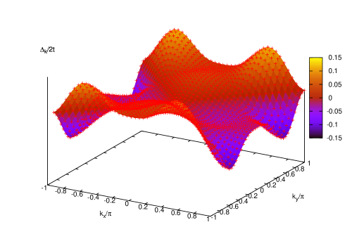
Figure 1: The superconducting gap function $\tilde{\Delta}_{\bf k}$ versus ${\bf k}$, as obtained from Eq. (44) for a square lattice with $N=40\times 40$ sites. The parameters are $\delta=0.08$, $t^{\prime}=0.4t$, $T=0$. Note that the gap function shows $d$-wave symmetry.

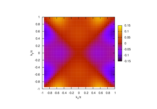
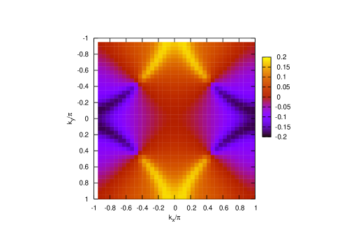
Figure 2: The superconducting gap $\tilde{\Delta}_{\bf k}$ (left panel) and the superconducting pairing function $\langle\hat{c}_{-{\bf k}\downarrow}\,\hat{c}_{{\bf k}\uparrow}\rangle$ for the same parameters as in Fig. 1 plotted as a 2d map.

IV.1.1 Zero temperature results

In Fig. 1, the superconducting gap function $\tilde{\Delta}_{\bf k}$ is plotted in ${\bf k}$-space for optimal doping, $\delta=0.08$. In agreement with experiment, the solution shows $d$-wave symmetry with nodal lines directed along the diagonals of the Brillouin zone from $(-\pi,-\pi)$ to $(\pi,\pi)$ and from $(\pi,-\pi)$ to $(-\pi,\pi)$. No $s$-wave like solutions were found.

In Fig. 2, both the superconduction gap function $\tilde{\Delta}_{\bf k}$ (left panel) and the pair correlation function $\langle\hat{c}_{-{\bf k}\downarrow}\,\hat{c}_{{\bf k}\uparrow}\rangle$ (right panel) are shown as a 2d-plot for the same parameter values as in Fig. 1. Again, in both functions, the nodal lines are clearly seen. Moreover, the absolute value of the pair correlation $|\langle\hat{c}_{-{\bf k}\downarrow}\,\hat{c}_{{\bf k}\uparrow}\rangle|$ has a pronounced maximum along the Fermi surface (FS). This behavior can easily be understood from Eq. (37). For ${\bf k}$-values close to the FS, ${\bf k}\approx{\bf k}_{F}$, where $\varepsilon_{\bf k}\leq{\cal O}(\tilde{\Delta}_{\bf k})$, the quantity $|\langle\hat{c}_{-{\bf k}\downarrow}\,\hat{c}_{{\bf k}\uparrow}\rangle|$ is of order ${\cal O}(1)$. In contrast, for ${\bf k}$-vectors away from the FS (with $\varepsilon_{\bf k}\gg{\cal O}(\tilde{\Delta}_{\bf k})$), the pair correlation function is of order ${\cal O}(\Delta/t)$. Note that the gap function $|\tilde{\Delta}_{\bf k}|$ has only a weak minimum at the Fermi surface. Additional weak maxima can be detected for the following ${\bf k}$-vectors: $(\pm\pi,\pm 0.55\pi)$, $(\pm 0.55\pi,\pm\pi)$, $(\pm 0.5\pi,0)$ and $(0,\pm 0.5\pi)$.

Fig. 3 shows the superconducting gap function $\tilde{\Delta}_{\bf k}$ on the Fermi surface as a function of the Fermi surface angle $\phi$ for three doping values, $\delta=0.05$ (underdoped case, blue line), $\delta=0.08$ (optimally doped, black line), and $\delta=0.12$ (overdoped, red line). The angle $\phi$ was already defined in paper I in the inset of Fig. 3. In all three cases, $\tilde{\Delta}_{\bf k}$ shows a characteristic overall increase from the nodal ($\phi=0$) to the anti-nodal point. Note, however, that the maximum value is already reached at a finite angle of about $27^{\circ}$, which is followed by a weak decrease of $\tilde{\Delta}_{\bf k}$.

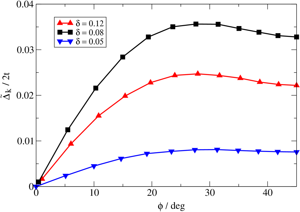
Figure 3: Superconducting gap function $\tilde{\Delta}_{\bf k}$ (in units of $2t$) as a function of the Fermi surface angle $\phi$ which was defined in the inset of Fig. 3 of paper I for three doping values, $\delta=0.05$ (underdoped case, blue line), $\delta=0.08$ (optimal doping, black line), and $\delta=0.12$ (overdoped case, red line).

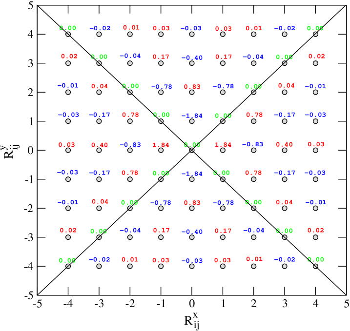
Figure 4: Superconducting order parameter in local space $\tilde{\Delta}_{ij}$ (in units of $10^{-2}(2t)$) for optimal doping $\delta=0.08$ and $T=0$. The hopping parameter $t^{\prime}$ between next-nearest neighbors is given by $t^{\prime}=0.4t$. $R_{ij}^{x}$ and $R_{ij}^{y}$ denote the $x$ and $y$ components of ${\bf R}_{i}-{\bf R}_{j}$.

According to Fig. 1, the gap function shows a pronounced ${\bf k}$-dependence in the whole Brillouin zone. By Fourier transforming $\tilde{\Delta}_{\bf k}$ to the local space,

$$\tilde{\Delta}_{ij} = \frac{1}{N}\sum_{i,j}\tilde{\Delta}_{\bf k}^{(\infty)}\,e^{i{\bf k}({\bf R}_{i}-{\bf R}_{j})}\,,$$ (38)

one finds the spatial dependence shown in Fig. 4. The figure again reveals the $d$-wave character of the superconducting order parameter. Note that the strong ${\bf k}$-dependence of $\tilde{\Delta}_{\bf k}$ maps on a short range behavior in local space. As is clearly seen, the local order parameter decays in space within a few lattice constants. This feature is consistent with the experimentally found superconducting coherence length in the cuprates of the order of a few lattice constants. The order parameter changes its sign by proceeding along the $x$- or $y$-axis. This can be seen for various hole fillings in Fig. 5, where $\tilde{\Delta}_{ij}$ is shown as a function of $R_{ij}^{x}$ (for fixed $R_{ij}^{y}=0$). Here $R_{ij}^{x}$ and $R_{ij}^{y}$ are the components of the difference vector ${\bf R}_{ij}={\bf R}_{i}-{\bf R}_{j}$ between lattice sites ${\bf R}_{i}$ and ${\bf R}_{j}$. The alternating sign of $\tilde{\Delta}_{ij}$ seems to be reminiscent of the sign behavior of antiferromagnetic correlations. However, the sign change is a property of the superconducting state and not of antiferromagnetic correlations.

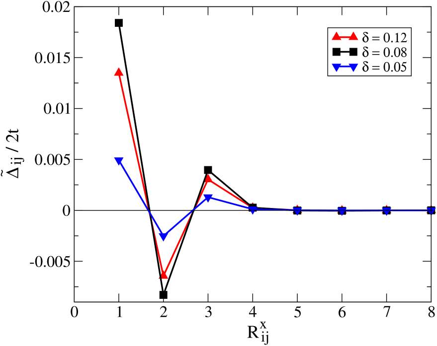
Figure 5: Superconducting order parameter $\tilde{\Delta}_{ij}$ (in units of $2t$) in local space along the $x$ direction (for $R_{ij}^{y}=0$) for three different hole fillings $\delta=0.05$ (blue), $0.08$ (black), and $0.12$ (red). The parameters $t^{\prime}$ and $T$ are the same as in Fig. 1.

IV.1.2 Finite temperature results

In Fig. 6, the local order parameter $\tilde{\Delta}_{ij}$ is plotted as a function of $T$ for different values of the distance between local sites, $\kappa=|{\bf R}_{ij}|$. The curves are obtained from Fourier back transforming Eq. (38) together with the temperature dependent expression for $\langle\hat{c}_{-{\bf k}\downarrow}\hat{c}_{{\bf k}\uparrow}\rangle$ from Sec. III.2. All curves vanish at the same temperature $T/2t\approx 0.026$, which defines the critical temperature $T_{c}$. Note that the temperature dependence of $\tilde{\Delta}_{ij}$ and thus of the gap function $\tilde{\Delta}_{\bf k}$ resembles that of the order parameter in BCS superconductors. This property can be traced back to the diagonalization approach on the basis of a Bogoliubov transformation in Appendix B, which is applied to the renormalized Hamiltonian $\tilde{\cal H}$ in the superconducting state. Also the pair correlation function $\langle\hat{c}_{-{\bf k}\downarrow}\hat{c}_{{\bf k}\uparrow}\rangle$ is evaluated in this way which results in a temperature dependence as in BCS superconductors as well.

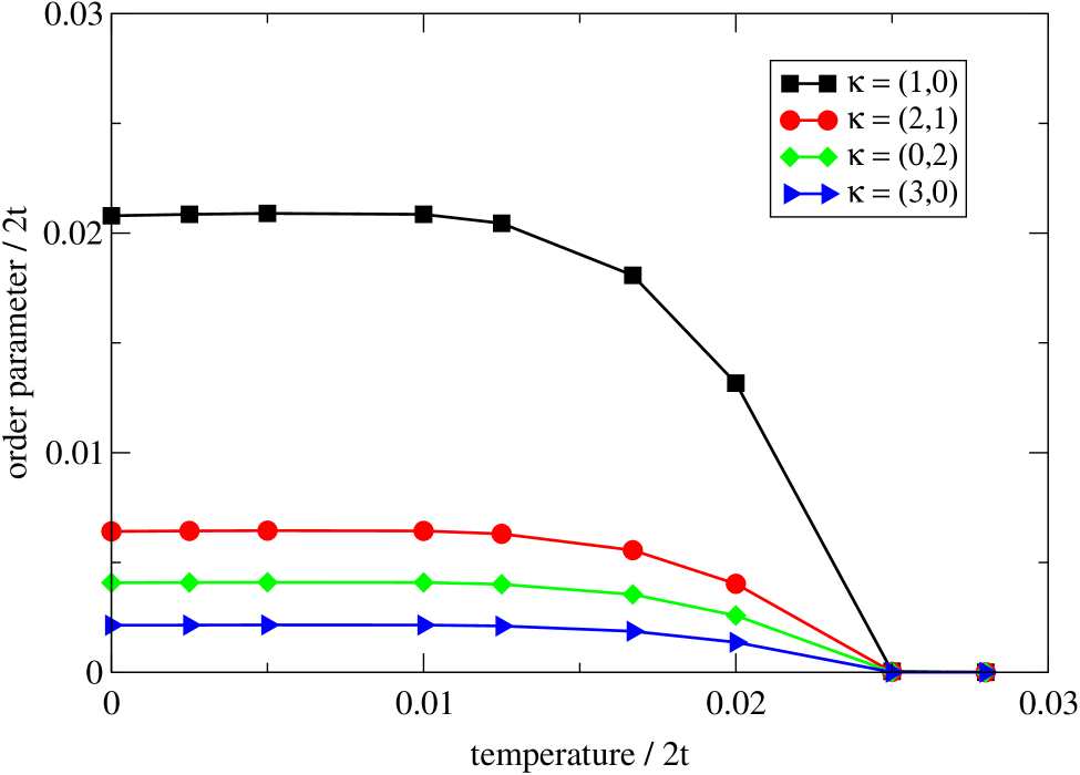
Figure 6: Local order parameter $\tilde{\Delta}_{ij}(T)$ as function of $T$ (both in units of $2t$) for different values of the distance $\kappa=|{\bf R}_{ij}|$. Note that all curves vanish at the same critical temperature $T_{c}$.

In Fig. 7, the critical temperature $T_{c}$ is given as a function of the hole doping $\delta$. The parameter values are again $t^{\prime}=0.4t$ and $J=0.2t$. Note that for small hole doping $\delta\leq 0.03$, no superconducting solutions are found. Also this result of the PRM is in good agreement with experiments. In the underdoped region for $\delta>0.03$, the critical temperature $T_{c}$ first increases substantially until it arrives a maximum value at about $\delta\approx 0.08$. Above the optimal doping concentration of $\delta=0.08$, the critical temperature decreases again (overdoped region). Within the parameter range, given in the figure, the $T_{c}$ behavior agrees very well with experiment. For still larger values of $\delta$ ($\delta>0.15$), our PRM result for $T_{c}$ remains finite. This feature is in disagreement with experiments, where the superconducting phase vanishes above a critical hole concentration. However, this defect of the present approach is by no means surprising. As was discussed in Sec. III, we have argued from the beginning that the present approach is not applicable for the case of large hole doping. Nevertheless, Fig. 7 demonstrates that we are able to explain the experimental findings at least in the underdoped and in the optimal doping regime. For the present parameter values, the maximum of $T_{c}$ at optimal doping is approximately given by $T_{c}\approx 0.06t$. Assuming a bare bandwidth of $8t\approx 10^{4}K$, this $T_{c}$-value corresponds to a critical temperature of order $50-100K$, which is in the correct order of magnitude.

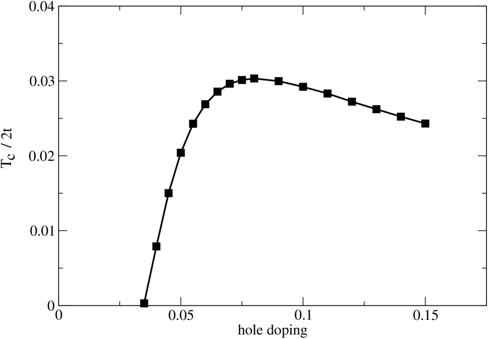
Figure 7: Critical temperature $T_{c}$ as a function of the hole doping $\delta$ for $t^{\prime}=0.4t$ and $J=0.2t$. No superconducting solution is found for $\delta\leq 0.03$. This result explains the vanishing of the superconducting phase in the cuprates at very low doping.

IV.1.3 Discussion

Next, we want to discuss the origin of the superconducting pairing mechanism. Let us start with the superconducting order parameter $\tilde{\Delta}_{\bf k}^{(1)}$ after the first renormalization step. According to Eq. (III.1), we have

$$\tilde{\Delta}_{{\bf k}}^{(n=1)} = {\Delta}_{{\bf k},\lambda=0}-\frac{1}{N}\sum_{\bf q}\frac{3J_{\bf q}}{4\hat{\omega}^{2}_{{\bf q},\lambda=0}}(\varepsilon_{{\bf k},\lambda=0}-\varepsilon_{{\bf k}+{\bf q},\lambda=0})^{2}\,\langle\hat{c}_{-({\bf k}+{\bf q})\downarrow}\,\hat{c}_{{\bf k}+{\bf q}\uparrow}\rangle.$$ (39)

The first term on the right hand side results from second order renormalization contributions according to Eq. (17). The numerical evaluation of Eq. (39) shows that it is small compared to the second term. According to Sec. III, the latter one results from the factorization of the contribution $\sim\dot{\bf S}_{\bf q}\dot{\bf S}_{-{\bf q}}$ in the renormalized Hamiltonian ${\cal H}_{\lambda=0}=\sum_{\bf q}({J_{\bf q}})/({2\hat{\omega}_{\bf q}^{2}})\dot{\bf S}_{\bf q}\dot{\bf S}_{-{\bf q}}+\cdots$ after the first renormalization cycle. Therefore, we can conclude from (48) that the dominant part of the microscopic pairing interaction is given by

$${\cal H}_{(SC)} = \frac{1}{N}\sum_{{\bf q}{\bf k}}\frac{J_{\bf q}}{4\hat{\omega}_{\bf q}^{2}}(\varepsilon_{\bf k}-\varepsilon_{{\bf k}-{\bf q}})^{2}\big{(}\hat{c}_{{\bf k}\uparrow}^{\dagger}\hat{c}_{-{\bf k}\downarrow}^{\dagger}\hat{c}_{-({\bf k}-{\bf q})\downarrow}\hat{c}_{{\bf k}-{\bf q}\uparrow}+2\hat{c}_{{\bf k}\uparrow}^{\dagger}\hat{c}_{-{\bf k}\downarrow}^{\dagger}\hat{c}_{{\bf k}-{\bf q}\downarrow}\hat{c}_{-({\bf k}-{\bf q})\uparrow}\big{)}\,.$$ (40)

Here, spin-singlet pairing was assumed. The expression (40) is our central result for the superconducting pairing mechanism in the cuprates. In contrast to usual BCS superconductors, where the pairing interaction between Cooper electrons is mediated by phonons, the present result can not be interpreted as an effective interaction of second order in some electron-bath coupling. Note that Eq. (40) results from the part of the exchange ${\cal H}_{J}$ which commutes with ${\cal H}_{t}$. An important feature of the pairing interaction is the oscillation frequency $\hat{\omega}_{\bf q}^{2}$ in the denominator of Eq. (40),

$$\hat{\omega}^{2}_{\bf q} = -2P_{0}(t^{2}_{{\bf q}=0}-t^{2}_{{\bf q}})=\hat{\omega}^{2}_{-{\bf q}}\geq 0,\quad\qquad t^{2}_{\bf q}=\sum_{l(\neq i)}t_{il}^{2}\,\cos{{\bf q}({\bf R}_{l}-{\bf R}_{i})}\,,$$ (41)

which enhances the pairing mechanism for small hole doping, since $P_{0}\sim\delta$. Therefore, the pairing interaction is mediated by oscillating hopping processes between nearest neighbors. This was discussed in detail in Sec. IV A of paper I. First, an electron hops to a neighboring site which is empty. In the second step, it hops back to the first site, since this site was certainly empty after the first hop. Thereby, the presence of short range antiferromagnetic correlations in the unperturbed Hamiltonian ${\cal H}_{0}$ is crucial, since it prevents the hopping to more distant sites.

In order to derive an approximate gap equation, let us again start from Eq. (39). When we restrict ourselves to a weak coupling theory, the $\lambda$-dependence of $\varepsilon_{{\bf k},\lambda}$ and $\hat{\omega}_{{\bf q},\lambda}$ can be neglected:

$$\tilde{\Delta}_{{\bf k}}^{(1)} = -\frac{1}{N}\sum_{\bf q}\frac{3J_{\bf q}}{4\hat{\omega}^{2}_{\bf q}}(\varepsilon_{\bf k}-\varepsilon_{{\bf k}+{\bf q}})^{2}\,\langle\hat{c}_{-({\bf k}+{\bf q})\downarrow}\,\hat{c}_{{\bf k}+{\bf q}\uparrow}\,\rangle\,,$$ (42)

where the first term from Eq. (39) was already omitted. For a purely qualitative discussion of the gap parameter, let us abandon all higher order renormalization effects, which would be included in the full renormalization scheme of Sec. III. Inserting the former expression (III.2.2) for $\langle\hat{c}_{-{\bf k}\downarrow}\hat{c}_{{\bf k}\uparrow}\rangle$ into Eq. (42), we find

$$\tilde{\Delta}_{{\bf k}}^{(1)} = -\frac{1}{N}\sum_{\bf q}\frac{3J_{\bf q}}{4\hat{\omega}^{2}_{\bf q}}(\varepsilon_{\bf k}-\varepsilon_{{\bf k}+{\bf q}})^{2}\,\tilde{u}_{{\bf k}+{\bf q}}^{2}D^{2}\frac{1-2f(E_{{\bf k}+{\bf q}})}{2\sqrt{\varepsilon_{{\bf k}+{\bf q}}^{2}+D^{2}\tilde{\Delta}_{{\bf k}+{\bf q}}^{2}}}\tilde{\Delta}_{{\bf k}+{\bf q}},$$ (43)

where $E_{\bf k}$ is again given by $E_{\bf k}=\sqrt{\varepsilon_{\bf k}^{2}+D^{2}\tilde{\Delta}_{\bf k}^{2}}$, and $f(E_{\bf k})$ is the Fermi function $f(E_{\bf k})=1/(1+e^{\beta E_{\bf k}})$. Moreover, by replacing on the left hand side also $\tilde{\Delta}_{\bf k}^{(1)}$ by $\tilde{\Delta}_{\bf k}$, we arrive at the following approximate gap equation

$$\tilde{\Delta}_{{\bf k}} \approx -\frac{1}{N}D^{2}\sum_{\bf q}\frac{3J_{\bf q}}{4\hat{\omega}^{2}_{{\bf q}}}(\varepsilon_{{\bf k}}-\varepsilon_{{\bf k}+{\bf q}})^{2}\,\tilde{u}_{{\bf k}+{\bf q}}^{2}\frac{1-2f(E_{{\bf k}+{\bf q}})}{2\sqrt{\varepsilon_{{\bf k}+{\bf q}}^{2}+D^{2}\tilde{\Delta}_{{\bf k}+{\bf q}}^{2}}}\tilde{\Delta}_{{\bf k}+{\bf q}}.$$ (44)

Note that the main features of our numerical results for the full renormalization scheme can already be detected from this equation. Due to the doping dependence of $\tilde{u}_{\bf k}$, shown in Fig. 9 of paper I, superconductivity sets in at the same small $\delta$-value, at which $\tilde{u}_{\bf k}$ becomes non-zero. With increasing hole doping, $\tilde{u}_{\bf k}$ increases, which also leads to a strengthening of the coherent excitation in $\Im G({\bf k},\omega)$. Moreover, superconductivity is favored for low doping due to the factor $\hat{\omega}^{2}_{\bf q}\sim\delta$ in the denominator of Eq. (44). Both features together, i.e. the increase of $\tilde{u}_{\bf k}$ with $\delta$ and $\hat{\omega}^{2}_{\bf q}\sim\delta$ lead to a maximum of $T_{c}$ at a finite doping value which is seen in Fig. 7. The property $\hat{\omega}^{2}_{\bf q}\sim\delta$ also explains the decrease of $T_{c}$ in the overdoped region, since renormalization processes become weaker for larger $\delta$.

The preference of the PRM to find solutions with $d$-wave symmetry for the gap parameter can also be understood from the gap equation (44). For an explanation, let us start by dividing the sum over $\bf q$ in Eq. (44) into two parts with $|\varepsilon_{{\bf k}+{\bf q}}|\leq|\tilde{\Delta}_{{\bf k}+{\bf q}}|$ and $|\varepsilon_{{\bf k}+{\bf q}}|>|\tilde{\Delta}_{{\bf k}+{\bf q}}|$. Omitting the second sum, one finds

$$\tilde{\Delta}_{{\bf k}} \approx -\frac{1}{N}\,\sum_{{\bf q},|\varepsilon_{{\bf k}+{\bf q}}|\leq|\tilde{\Delta}_{{\bf k}+{\bf q}}|}\frac{3J_{\bf q}}{4\hat{\omega}^{2}_{\bf q}}\,(\varepsilon_{\bf k}-\varepsilon_{{\bf k}+{\bf q}})^{2}\,\tilde{u}_{{\bf k}+{\bf q}}^{2}D^{2}\frac{1-2f(E_{{\bf k}+{\bf q}})}{2\sqrt{\varepsilon_{{\bf k}+{\bf q}}^{2}+\tilde{\Delta}_{{\bf k}+{\bf q}}^{2}}}\,\tilde{\Delta}_{{\bf k}+{\bf q}}.$$ (45)

For most values of ${\bf k}$, the neglected sum is smaller by a factor of order $\Delta/t$. An exception are ${\bf k}$-values close to the Fermi surface ${\bf k}\approx{\bf k}_{F}$ (with $|\varepsilon_{\bf k}|\leq O(\Delta_{\bf k})$), which will be excluded in the following discussion. Here, the sum with $|\varepsilon_{{\bf k}+{\bf q}}|>|\tilde{\Delta}_{{\bf k}+{\bf q}}|$ would be larger by a factor of order $t/\Delta$. With respect to Eq. (45), those terms of the ${\bf q}$ sum are most important, which have energies $|\varepsilon_{{\bf k}+{\bf q}}|$ not exceeding $|\tilde{\Delta}_{{\bf k}+{\bf q}}|$. For ${\bf k}$-values on the diagonal, $k_{x}=k_{y}$, of the Brillouin zone, it can be seen that ${\bf q}$-values with $q_{y}\approx q_{x}\pm\pi$ lead to small energies $\varepsilon_{{\bf k}+{\bf q}}\approx 0$ and thus to the dominant contributions in Eq. (45). Here, the dispersion relation $\varepsilon_{\bf k}=-2t(\cos{k_{x}a}+\cos{k_{y}a})$ was used. However, the prefactor $J_{\bf q}$ vanishes in this case. This explains the nodal line $k_{x}=k_{y}$ and similarly $k_{x}=-k_{y}$ of the gap parameter in Fig. 2. However note that the exchange constant $J_{\bf q}$ changes its sign as a function of $\bf q$. From this behavior, one can conclude that $d$-wave symmetry for the order parameter is more favorable than $s$-wave symmetry.

IV.2 ARPES Spectral functions

Finally, let us discuss the ARPES spectral function in the superconducting phase. This quantity is obtained from the dissipative part of the anticommutator Green function (28).

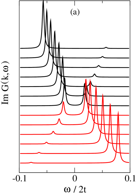
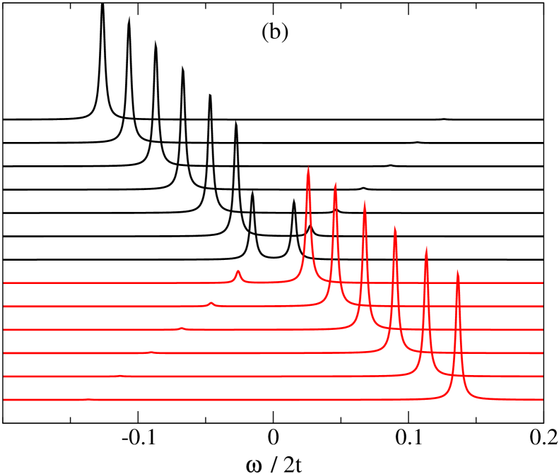
Figure 8: Spectral functions $\Im G({\bf k},\omega)$ in the superconducting phase at optimal doping, $\delta=0.08$ for two fixed $k_{x}$-values: (a) $k_{x}=\pi$ (anti-nodal region) and (b) $k_{x}=5\pi/8$ (in between anti-nodal and nodal region). By varying $k_{y}$ , the Fermi surface is crossed. The other parameters are $t^{\prime}=0.4t$, $J=0.2t$, and $T=0$.

In Figs. 8 - 10, our results for the superconducting phase are given which are obtained from the numerical evaluation of Eq. (III.2.1). First, in Fig. 8, we have chosen as parameters: $\delta=0.08$ (optimal doping), $T=0$, $t^{\prime}=0.4t$, and $J=0.2t$. Two cuts with fixed $k_{x}$ and varying $k_{y}$ are shown. Thereby the FS is crossed. In panel (a), where $k_{x}=\pi$, the spectra belong to ${\bf k}$-values in the anti-nodal region, whereas in (b) $k_{x}=5\pi/8$. Here, a ${\bf k}$-region is probed in-between the nodal and the anti-nodal point. The spectra in both panels display peak-like structures in a small energy range around $\omega=0$. Note that all structures are caused alone by the coherent part of $\Im G({\bf k},\omega)$ (first line in Eq. (III.2.1)), which consists of two peaks at the positions $\omega=\pm E_{\bf k}$. For ${\bf k}$-vectors, far away from the FS (top and bottom plots in Figs. 8(a) and (b)), a dominating peak at $\omega\approx\tilde{\varepsilon}_{\bf k}$ is found, which arises from the excitations at $\pm E_{\bf k}$, depending on the sign of $\tilde{\varepsilon}_{\bf k}$. By approaching the FS, a secondary peak arises at $\omega\approx-\tilde{\varepsilon}_{\bf k}$. An expansion of the prefactors in Eq. (III.2.1) shows that in each case the secondary peak has a smaller weight of order $(\tilde{\Delta}_{\bf k}/\tilde{\varepsilon}_{\bf k})^{2}$. Only for ${\bf k}$-values on the FS ($\tilde{\varepsilon}_{\bf k}=0$), the two coherent peaks have equal weight. They are separated by an energy distance, which is given by the gap parameter $(2D\tilde{\Delta}_{\bf k})$. Note that the gap size is almost the same for the two cases of Fig. 8.

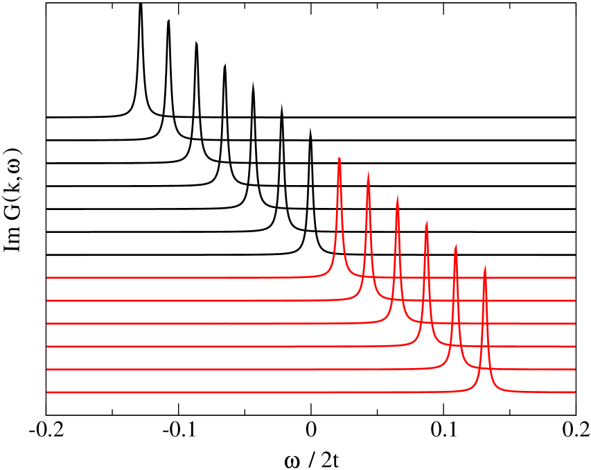
Figure 9: Spectral functions $\Im G({\bf k},\omega)$ as in Fig. 8 for a fixed $k_{x}$-value, $k_{x}=\pi/2$ . By varying $k_{y}$ the Fermi surface is crossed in the nodal region.

A comparison of both panels of Fig. 8 also shows that the secondary peak is more pronounced in the anti-nodal region than in-between the anti-nodal and nodal region. Furthermore, the overall dispersion of $\tilde{\varepsilon}_{\bf k}$ of the primary peak is weaker in the anti-nodal region than for the case of intermediate $k_{x}$-values. With respect to the incoherent contributions to $\Im G({\bf k},\omega)$, note that for optimal doping the overall weight of the coherent and of the incoherent excitations are approximately the same. However, the incoherent part of the spectrum is spread over a much larger frequency range. Therefore, in a small $\omega$-range, close to the Fermi level, the coherent excitations are dominant.

In Fig. 9, the spectral function is plotted in the nodal region for fixed $k_{x}=\pi/2$ and different values of $k_{y}$. Thereby, again the FS is crossed. Note that neither a secondary peak nor a superconducting gap is found in the nodal region. Also, the coherent peak moves almost unchanged through the FS, when $k_{y}$ is varied.

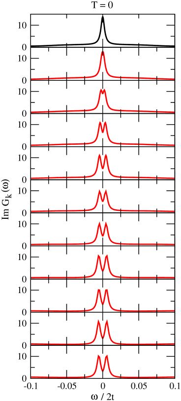
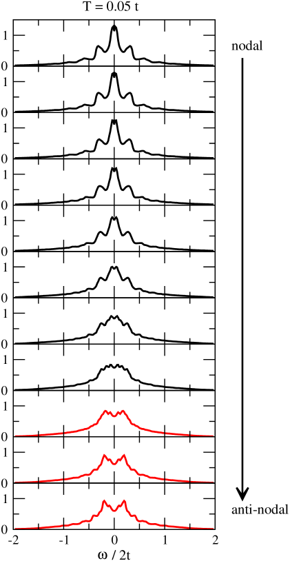
Figure 10: Symmetrized spectral functions $\Im G({\bf k},\omega)$ for ${\bf k}$-values on the FS between the nodal (top) and anti-nodal point (bottom) for two temperatures (a) in the superconducting phase at $T=0$, and (b) in the pseudogap phase at $T=0.05t$. The critical temperature is $T_{c}=0.03t$ (underdoped case $\delta=0.05$). The other parameters are the same as in Fig. 8.

Finally, Fig. 10 shows the results for the symmetrized spectral functions $\Im G({\bf k},\omega)$ for two different temperatures (a) $T=0$ (superconducting phase) and (b) $T=0.05t$ (pseudogap phase). The $\bf k$-values proceed on the FS between the nodal (top) and the anti-nodal (bottom) point. The hole concentration is $\delta=0.05$ (underdoped regime) which leads to a critical temperature $T_{c}=0.03t$. In the spectra at temperature $T=0$, one recognizes the opening of a superconducting gap for all $\bf k$-vectors except at the nodal point. The gap size as a function of the Fermi surface angle $\phi$ is given by the blue line in Fig. 3. Similar as before, the peak-like structure arises from the coherent excitations in a small $\omega$-range around $\omega=0$. For the higher temperature, $T=0.05t$ (pseudogap phase), the system is in the normal state. On a substantial part of the Fermi surface, the spectra now show the typical large spectral weight around $\omega=0$, indicating a Fermi arc of gapless excitations. The Fermi arc extents over a finite ${\bf k}$-range. In contrast to the superconducting case, the spectrum is now dominated by the incoherent excitations. In the anti-nodal region, they form the pseudogap around $\omega=0$ (see also paper I). Note that the pseudogap in Fig. 10(b) is about ten times larger than the superconducting gap at $T=0$ (for the present hole doping $\delta=0.05$). Note that for both temperatures, the spectra are in good qualitative agreement with recent ARPES measurementsK06 ,K07 ,K08 .

Let us finally make one remark concerning the linewidth of the coherent peaks. As was already mentioned in Sec. V of paper I, from the experimental point of view, we would expect a temperature dependent broadening of the coherent peaks which is caused by the coupling to other degrees of freedom. Such a broadening was not incorporated in the present approach. Note, however, that a broadening of the spectra is also produced by the incoherent excitations of $\Im G({\bf k},\omega)$. In order to include a temperature dependent broadening of the coherent excitations, we have added by hand a small linewidth in Fig. 10, which is taken of the order of $k_{B}T$.

V Conclusions

In this paper, we have given a microscopic approach to the superconducting phase in cuprate systems at moderate hole doping. Thereby, a recently developed projector-based renormalization method (PRM) was applied to the $t$-$J$ model. Our result for the superconducting order parameter shows $d$-wave symmetry with a coherence length of a few lattice constants which is in agreement with experiments. In contrast to usual BCS superconductors, where the pairing interaction between Cooper electrons is mediated by phonons, the superconducting pairing interaction in the cuprates can not be interpreted as an effective interaction of second order in some electron-bath coupling. Instead, the main contribution to the pairing results from the part of the exchange interaction which commutes with the hopping Hamiltonian ${\cal H}_{t}$. The superconducting state naturally arises from a typical oscillation behavior of the correlated electrons between neighboring lattice sites due to the presence of spin fluctuations. The theoretical results can explain the experimental findings in the underdoped as well as in the optimal doping regime. The obtained value of $T_{c}$ at optimal doping has the correct order of magnitude.

VI Acknowledgments

We would like to acknowledge stimulating and enlightening discussions with J. Fink and A. Hübsch. This work was supported by the DFG through the research program SFB 463.

Appendix A Factorization approximation for $\dot{\bf S}_{\bf q}\dot{\bf S}_{-{\bf q}}$

The aim of this appendix is to simplify the operator product $\dot{\bf S}_{\bf q}\dot{\bf S}_{-{\bf q}}$ which enters the expressions (9) for ${\cal H}_{0,\lambda}$ and ${\cal H}_{1,\lambda}$. As in paper I, we start from the expression

$$\dot{\bf S}_{{\bf q}}\dot{\bf S}_{-{\bf q}}=\frac{1}{4N}\sum_{\alpha\beta}\sum_{\gamma\delta}(\vec{\sigma}_{\alpha\beta}\cdot\vec{\sigma}_{\delta\gamma})\sum_{i\neq j}t_{ij}(e^{i{\bf q}{\bf R}_{i}}-e^{i{\bf q}{\bf R}_{j}})\sum_{l\neq m}t_{lm}(e^{-i{\bf q}{\bf R}_{l}}-e^{-i{\bf q}{\bf R}_{m}})\,\hat{c}_{i\alpha}^{\dagger}\hat{c}_{j\beta}\hat{c}_{m\delta}^{\dagger}\hat{c}_{l\gamma}.$$

The four-fermion operator on the right hand side can be factorized in two different ways: One can either reduce it to operators $\hat{c}^{\dagger}_{{\bf k}\sigma}\hat{c}_{{\bf k}\sigma}$ or to operators $\hat{c}^{\dagger}_{{\bf k}\sigma}\hat{c}^{\dagger}_{-{\bf k},-\sigma}$ and $\hat{c}_{-{\bf k},-\sigma}\,\hat{c}_{{\bf k},\sigma}$. The first factorization will lead to a renormalization of $\varepsilon_{\bf k}$, whereas the second one renormalizes the superconducting order parameter $\Delta_{\bf k}$. In the factorization, we have to pay attention to the fact that the averaged spin operator vanishes $\langle{\bf S}_{i}\rangle=0$ outside the antiferromagnetic regime. Moreover, all local indices in the four-fermion term of (A) should be different from each other. This follows from the former decomposition of the exchange interaction into eigenmodes of ${\sf L}_{t}$, where we have implicitly assumed that the operators $\dot{\bf S}_{{\bf q}}$ and $\dot{\bf S}_{-{\bf q}}$ do not overlap in the local space. Otherwise, the decomposition would be much more involved. However, it can be shown that these ’interference’ terms only make a minor impact on the results.

(i) For the ’normal’ factorization, we find

$$\dot{\bf S}_{{\bf q}}\dot{\bf S}_{-{\bf q}}|_{(\mbox{\tiny i})}=-\frac{3}{2N}\sum_{{\bf k}\sigma}(\varepsilon_{\bf k}-\varepsilon_{{\bf k}-{\bf q}})^{2}\langle(\hat{c}_{{\bf k}-{\bf q}\alpha}^{\dagger}\hat{c}_{{\bf k}-{\bf q}\alpha})_{NL}\rangle\,(\hat{c}_{{\bf k}\sigma}^{\dagger}\hat{c}_{{\bf k}\sigma})_{NL}\,,$$ (47)

where we have defined $(\hat{c}_{{\bf k}\sigma}^{\dagger}\hat{c}_{{\bf k}\sigma})_{NL}=\hat{c}_{{\bf k}\sigma}^{\dagger}\hat{c}_{{\bf k}\sigma}-({1}/{N})\sum_{{\bf k}^{\prime}}\hat{c}_{{\bf k}^{\prime}\sigma}^{\dagger}\hat{c}_{{\bf k}^{\prime}\sigma}$. The attached subscript ${NL}$ indicates that the local sites of the operators inside the brackets are different from each other. In Eq. (47), we have also neglected an additional c-number quantity, which enters in the factorization, and the sums over the spin indices in Eq. (A) have already been carried out

(ii) By assuming spin-singlet pairing, we obtain from Eq. (A),

$$\dot{\bf S}_{{\bf q}}\dot{\bf S}_{-{\bf q}}|_{(\mbox{\tiny{ii}})} = \frac{1}{2N}\sum_{{\bf k}}(\varepsilon_{\bf k}-\varepsilon_{{\bf k}-{\bf q}})^{2}\big{(}\hat{c}_{{\bf k}\uparrow}^{\dagger}\hat{c}_{-{\bf k}\downarrow}^{\dagger}\hat{c}_{-({\bf k}-{\bf q})\downarrow}\hat{c}_{{\bf k}-{\bf q}\uparrow}+2\hat{c}_{{\bf k}\uparrow}^{\dagger}\hat{c}_{-{\bf k}\downarrow}^{\dagger}\hat{c}_{{\bf k}-{\bf q}\downarrow}\hat{c}_{-({\bf k}-{\bf q})\uparrow}\big{)}.$$ (48)

According to Sec. IV A, the expression (48) leads to the main part of the superconducting pair interaction. In a factorization approximation, the two contributions in (48) can be combined to

$$\dot{\bf S}_{{\bf q}}\dot{\bf S}_{-{\bf q}}|_{(\mbox{\tiny{ii}})}=\frac{3}{2N}\sum_{{\bf k}}(\varepsilon_{\bf k}-\varepsilon_{{\bf k}-{\bf q}})^{2}\left\{\langle\hat{c}_{-({\bf k}-{\bf q})\downarrow}\hat{c}_{{\bf k}-{\bf q}\uparrow}\rangle\,\,\hat{c}_{{\bf k}\uparrow}^{\dagger}\hat{c}_{-{\bf k}\downarrow}^{\dagger}+h.c.\right\}.$$ (49)

Using Eqs. (47) and (49) together with Eq. (22), one is finally led to the renormalization result (III.1) for $\tilde{\varepsilon}_{\bf k}^{(0)}$ and $\tilde{\Delta}_{\bf k}^{(0)}$ to first order in $J$.

The above factorization can also be used to derive the renormalization contributions (III.1),(17) to ${\varepsilon}_{{\bf k},\lambda-\Delta\lambda}$ and $\Delta_{{\bf k},\lambda-\Delta\lambda}$. Using the expressions (47) and (48), we can first simplify the second order renormalization ${\cal H}_{\lambda-\Delta\lambda}^{(2)}$ of ${\cal H}_{\lambda-\Delta\lambda}$. In analogy to the results of Appendix B in paper I, we arrive at

$${\cal H}_{\lambda-\Delta\lambda}^{(2)} = 3\sum_{\bf q}(\frac{J_{\bf q}}{4\hat{\omega}_{\bf q}^{2}})^{2}\,\Theta_{\bf q}(\lambda,\Delta\lambda)\left(\left[\frac{1}{N}\sum_{{\bf k}\sigma}(2\varepsilon_{\bf k}-\varepsilon_{{\bf k}+{\bf q}}-\varepsilon_{{\bf k}-{\bf q}})\langle\hat{c}_{{\bf k}\sigma}^{\dagger}\hat{c}_{{\bf k}\sigma}\rangle\right]\,{\bf S}_{\bf q}\cdot{\bf S}_{-{\bf q}}\right.$$ (50)

$$\left.\qquad+\langle{\bf S}_{\bf q}\cdot{\bf S}_{-{\bf q}}\rangle\,\frac{1}{N}\sum_{{\bf k}\sigma}(2\varepsilon_{\bf k}-\varepsilon_{{\bf k}+{\bf q}}-\varepsilon_{{\bf k}-{\bf q}})\;\hat{c}_{{\bf k}\sigma}^{\dagger}\hat{c}_{{\bf k}\sigma}\right)$$

$$- \sum_{\bf q}(\frac{J_{\bf q}}{4\hat{\omega}_{\bf q}^{2}})^{2}\,\Theta_{\bf q}(\lambda,\Delta\lambda)\langle\dot{\bf S}_{\bf q}\cdot\dot{\bf S}_{-{\bf q}}\rangle\,\frac{1}{N}\sum_{{\bf k}\sigma}(2\varepsilon_{\bf k}-\varepsilon_{{\bf k}+{\bf q}}-\varepsilon_{{\bf k}-{\bf q}})\;\hat{c}_{{\bf k}\sigma}^{\dagger}\hat{c}_{{\bf k}\sigma}$$

$$+ \frac{3}{2N}\sum_{{\bf q}\sigma}(\frac{J_{\bf q}}{4\hat{\omega}_{\bf q}^{2}})^{2}\,\Theta_{\bf q}(\lambda,\Delta\lambda)\,\left[\frac{1}{N}\sum_{{\bf k}^{\prime}\sigma^{\prime}}(2\varepsilon_{{\bf k}^{\prime}}-\varepsilon_{{\bf k}^{\prime}+{\bf q}}-\varepsilon_{{\bf k}^{\prime}-{\bf q}})\langle\hat{c}_{{\bf k}^{\prime}\sigma^{\prime}}^{\dagger}\hat{c}_{{\bf k}^{\prime}\sigma^{\prime}}\rangle\right]\times$$

$$\qquad\times\sum_{{\bf k}\sigma}(\varepsilon_{\bf k}-\varepsilon_{{\bf k}-{\bf q}})^{2}\langle(\hat{c}_{{\bf k}-{\bf q}\alpha}^{\dagger}\hat{c}_{{\bf k}-{\bf q}\alpha})_{NL}\rangle\,(\hat{c}_{{\bf k}\sigma}^{\dagger}\hat{c}_{{\bf k}\sigma})_{NL}$$

$$- \frac{1}{2N}\sum_{{\bf q}\sigma}(\frac{J_{\bf q}}{4\hat{\omega}_{\bf q}^{2}})^{2}\,\Theta_{\bf q}(\lambda,\Delta\lambda)\,\left[\frac{1}{N}\sum_{{\bf k^{\prime}}\sigma^{\prime}}(2\varepsilon_{{\bf k}^{\prime}}-\varepsilon_{{\bf k}^{\prime}+{\bf q}}-\varepsilon_{{\bf k}^{\prime}-{\bf q}})\langle\hat{c}_{{\bf k}^{\prime}\sigma^{\prime}}^{\dagger}\hat{c}_{{\bf k}^{\prime}\sigma^{\prime}}\rangle\right]\times$$

$$\qquad\times\sum_{\bf k}(\varepsilon_{\bf k}-\varepsilon_{{\bf k}-{\bf q}})^{2}\langle(\hat{c}_{{\bf k}-{\bf q}\downarrow}\hat{c}_{{\bf k}-{\bf q}\uparrow})\rangle\,(\hat{c}_{{\bf k}\uparrow}^{\dagger}\hat{c}_{{\bf k}\downarrow}^{\dagger}+h.c.).$$

From (50), the second order renormalizations to $\varepsilon_{{\bf k},\lambda-\Delta\lambda}$ and $\Delta_{{\bf k},\lambda-\Delta\lambda}$ can immediately be deduced.

Appendix B Bogoliubov transformation for the superconducting Hamiltonian $\tilde{\cal H}$

The aim of this appendix is to diagonalize the renormalized Hamiltonian $\tilde{\cal H}$ for the superconducting phase. According to Eq. (25), the Hamiltonian $\tilde{\cal H}$ reads

$$\tilde{\cal H} = \sum_{{\bf k}\sigma}\tilde{\varepsilon}_{\bf k}\,\hat{c}_{{\bf k}\sigma}^{\dagger}\,\hat{c}_{{\bf k}\sigma}-\sum_{\bf k}\left(\tilde{\Delta}_{{\bf k}}\,\hat{c}_{{\bf k},\uparrow}^{\dagger}\hat{c}_{-{\bf k},\downarrow}^{\dagger}+\tilde{\Delta}_{{\bf k}}^{*}\,\hat{c}_{-{\bf k},\downarrow}\hat{c}_{{\bf k},\uparrow}\right)+\tilde{E}.$$ (51)

Due to the presence of the Hubbard operators in Eq. (51), the usual Bogoliubov transformation can only be applied approximately. Let us start by introducing new fermion operators,

$$\alpha_{\bf k}^{\dagger} = {\sf U}_{\bf k}\,\hat{c}_{{\bf k},\uparrow}^{\dagger}-{\sf V}_{\bf k}\,\hat{c}_{-{\bf k},\downarrow},$$ (52)

$$\beta_{\bf k}^{\dagger} = {\sf U}_{\bf k}\,\hat{c}_{-{\bf k},\downarrow}^{\dagger}+{\sf V}_{\bf k}\,\hat{c}_{{\bf k},\uparrow}.$$

We require that $\alpha_{\bf k}^{\dagger}$ and $\beta_{\bf k}^{\dagger}$ are eigenmodes of $\tilde{\cal H}$,

$$\tilde{\sf L}\alpha_{\bf k}^{\dagger} = E_{\bf k}\alpha_{\bf k}^{\dagger}\,,\quad\tilde{\sf L}\beta_{\bf k}^{\dagger}=E_{\bf k}\beta_{\bf k}^{\dagger}.$$ (53)

In order to find equations for ${\sf U}_{\bf k}$ and ${\sf V}_{\bf k}$, let us insert the expression (52) for $\alpha_{\bf k}^{\dagger}$ into the first equation of (53),

$${\sf U}_{\bf k}\,\tilde{\sf L}\hat{c}_{{\bf k},\uparrow}^{\dagger}-{\sf V}_{\bf k}\,\tilde{\sf L}\hat{c}_{-{\bf k},\downarrow} = E_{\bf k}\left({\sf U}_{\bf k}\,\hat{c}_{{\bf k},\uparrow}^{\dagger}-{\sf V}_{\bf k}\,\hat{c}_{-{\bf k},\downarrow}\right).$$ (54)

The two commutators on the left hand side of Eq. (54) will be evaluated separately. For the first one, $\tilde{\sf L}\hat{c}_{{\bf k}\sigma}=[\tilde{\cal H},\hat{c}_{{\bf k},\uparrow}^{\dagger}]$, we obtain:

$$\tilde{\sf L}\hat{c}_{{\bf k},\uparrow}^{\dagger} = \tilde{\sf L}_{t}\hat{c}_{{\bf k},\uparrow}^{\dagger}-\sum_{{\bf k}^{\prime}}\tilde{\Delta}_{{\bf k}^{\prime}}^{*}[\hat{c}_{-{\bf k}^{\prime},\downarrow}\hat{c}_{{\bf k}^{\prime},\uparrow},\hat{c}_{{\bf k},\uparrow}^{\dagger}].$$

Here, the Liouville operator $\tilde{\sf L}_{t}$ corresponds to the commutator with the hopping Hamiltonian $\tilde{\cal H}_{t}=\sum_{\bf k}\tilde{\varepsilon}_{\bf k}\,\hat{c}_{{\bf k}\sigma}^{\dagger}\hat{c}_{{\bf k}\sigma}$, which agrees with the fully renormalized Hamiltonian $\tilde{\cal H}$ in the normal state investigated in paper I. Therefore, we can use $\tilde{\sf L}_{t}\hat{c}_{{\bf k},\uparrow}^{\dagger}=\tilde{\varepsilon}_{\bf k}\,\hat{c}_{{\bf k}\sigma}^{\dagger}$ and find using the anti-commutator relation (2)

$$\tilde{\sf L}\hat{c}_{{\bf k},\uparrow}^{\dagger} = \tilde{\varepsilon}_{\bf k}\hat{c}_{{\bf k},\uparrow}^{\dagger}-\frac{1}{\sqrt{N}}\sum_{i\neq j}\tilde{\Delta}_{i,j}^{*}\left(e^{-i{\bf k}{\bf R}_{j}}{\cal D}_{\uparrow}(j)\,\hat{c}_{i,\downarrow}-e^{-i{\bf k}{\bf R}_{i}}S_{i}^{-}\hat{c}_{j,\uparrow}\right)\,.$$ (55)

The quantity $\tilde{\Delta}_{i,j}^{*}$ is defined by $\tilde{\Delta}_{i,j}^{*}=\frac{1}{N}\sum_{\bf k}\tilde{\Delta}_{\bf k}^{*}e^{i{\bf k}({\bf R}_{i}-{\bf R}_{j})}$, and ${\cal D}_{\sigma}(j)=1-n_{j,-\sigma}={\cal P}_{0}+\hat{n}_{i\sigma}$ was already given in Eq. (2). The main contribution to the second term in Eq. (55) is caused by the following process: First, two holes are generated at sites $i$ and $j$ before the hole at $j$ is annihilated again by a local creation operator in $\hat{c}_{{\bf k}\uparrow}^{\dagger}$. The arising local projector ${\cal D}_{\sigma}(i)$ will be approximated by its average $D=\langle{\cal D}_{\sigma}(j)\rangle=1-\langle n_{j,-\sigma}\rangle$. Thus, we obtain

$$\tilde{\sf L}\hat{c}_{{\bf k},\uparrow}^{\dagger} = \tilde{\varepsilon}_{\bf k}\hat{c}_{{\bf k},\uparrow}^{\dagger}-\frac{D}{\sqrt{N}}\sum_{i\neq j}\tilde{\Delta}_{i,j}^{*}e^{-i{\bf k}{\bf R}_{j}}\hat{c}_{i,\downarrow}$$ (56)

$$= \tilde{\varepsilon}_{\bf k}\hat{c}_{{\bf k},\uparrow}^{\dagger}-D\tilde{\Delta}_{\bf k}^{*}c_{-{\bf k},\downarrow}\,,$$

where $\tilde{\Delta}_{i,j}^{*}$ was Fourier back transformed to $\tilde{\Delta}_{\bf k}^{*}$. A corresponding contribution from the last term in Eq. (55) vanishes, since $\langle S_{i}^{-}\rangle=0$ outside the antiferromagnetic regime. The evaluation of the second commutator in Eq. (54) can be done in analogy to the result (56),

$$\tilde{\sf L}\hat{c}_{-{\bf k},\downarrow} = -\tilde{\varepsilon}_{\bf k}\hat{c}_{-{\bf k},\downarrow}-D\tilde{\Delta}_{\bf k}c_{{\bf k},\uparrow}^{\dagger}.$$ (57)

Inserting Eqs. (56) and (57) into Eq. (54) leads to the following two equations for ${\sf U}_{\bf k}$ and ${\sf V}_{\bf k}$:

$${\sf U}_{\bf k}\left(\tilde{\varepsilon}_{\bf k}-E_{\bf k}\right)+{\sf V}_{\bf k}D\tilde{\Delta}_{\bf k} = 0,$$

$$-{\sf U}_{\bf k}D\tilde{\Delta}_{\bf k}^{*}+{\sf V}_{\bf k}\left(\tilde{\varepsilon}_{\bf k}+E_{\bf k}\right) = 0.$$ (58)

The eigenvalue $E_{\bf k}$ for this system of equations is easily obtained:

$$E_{\bf k}=\sqrt{\tilde{\varepsilon}_{\bf k}^{2}+D^{2}|\tilde{\Delta}_{\bf k}|^{2}}.$$ (59)

The expectation value $\langle\hat{c}_{{\bf k},\uparrow}^{\dagger}\hat{c}_{-{\bf k},\downarrow}\rangle_{\tilde{\cal H}}$, formed with the superconducting Hamiltonian $\tilde{\cal H}$, is found by solving (52) for $\hat{c}_{{\bf k},\uparrow}^{\dagger}$ and $\hat{c}_{-{\bf k},\downarrow}$. Using the property (53), one finds

$$\left\langle\hat{c}_{{\bf k},\uparrow}^{\dagger}\hat{c}_{-{\bf k},\downarrow}^{\dagger}\right\rangle_{\tilde{\cal H}} = \frac{D^{2}\tilde{\Delta}_{\bf k}^{*}}{2E_{\bf k}}\left(1-\frac{2}{1+e^{\beta E_{\bf k}}}\right).$$ (60)

References

• (1) J.G. Bednorz and K.A. Müller, Z. Phys. B 64, 189 (1986).
• (2) J. Corson et al., Nature 398, 221 (1999).
• (3) V.J. Emery and S.A. Kivelson, Nature 374, 434-437 (1995).
• (4) D. Pines, Physica C 282287, 273 (1997).
• (5) M. Randeria, cond-mat 9710223 (1997).
• (6) C.M. Varma, Phys. Rev. B 55, 14554 (1997).
• (7) M.R. Norman et.al., Nature (London) 392, 157 (1998).
• (8) K.M: Shen et al.. Science 307, 901 (2005).
• (9) K. Terashima et al., Phys. Rev. Lett. 99, 017003 (2007).
• (10) A. Kanigel et al., Nature Phys. 2, 447 (2006).
• (11) A. Kanigel et al., Phys. Rev. Lett. 99, 157001 (2007).
• (12) A. Kanigel et al., Phys. Rev. Lett. 101, 137002 (2008).
• (13) S. Sykora and K.W. Becker, cond-mat 0903.0921 (2009).
• (14) K.W. Becker et al., Phys. Rev. B 66, 235115 (2002); for a review see A. Hübsch et al., cond-mat 0809.3360 (2008).
• (15) P. Fazekas in Lecture Notes on Electron Correlations and Magnetism, World Scientific, Singapore, New Jersey, London, Hongkong, 1999.
• (16) J.L: Tallon and J.W. Loram, Physica 249C, 53 (2001).