Influence on observation from IR divergence during inflation
— Single field inflation —

Abstract

A naive computation of the correlation functions of fluctuations generated during inflation suffers from logarithmic divergences in the infrared (IR) limit. In this paper, we propose one way to solve this IR divergence problem in the single-field inflation model. The key observation is that the variables that are commonly used in describing fluctuations are influenced by what we cannot observe. Introducing a new perturbation variable which mimics what we actually observe, we propose a new prescription to solve the time evolution of perturbation in which this leakage of information from the unobservable region of the universe is shut off. We give a proof that IR divergences are absent as long as we follow this new scheme. We also show that the secular growth of the amplitude of perturbation is also suppressed, at least, unless very higher order perturbation is discussed.

I Introduction

Inflation has become the leading paradigm to explain the seed of inhomogeneities of the universe as seen in the Cosmic Microwave Background (CMB). Despite its attractive aspects, there are still many unknown aspects about inflation scenario Lidsey:1995np ; Bassett:2005xm ; Lyth:2007qh ; Linde:2007fr . When we discuss the primordial fluctuations within linear analysis, many inflation models predict almost the same results, which are compatible with the observational data, although the underlying models are quiet different. To discriminate between different inflationary models, it is important to take into account nonlinear effects Bartolo:2001cw ; Bartolo:2004if ; Maldacena:2002vr ; Kim:2006te ; Babich:2004gb ; Seery:2005wm ; Seery:2005gb ; Weinberg:2005vy ; Weinberg:2006ac ; Rigopoulos:2005xx ; Rigopoulos:2005ae ; Rigopoulos:2005us ; Vernizzi:2006ve ; Chen:2006nt ; Battefeld:2006sz ; Yokoyama:2007dw ; Yokoyama:2008by ; Seery:2008ax ; Naruko:2008sq ; Weinberg:2008mc ; Weinberg:2008nf ; Weinberg:2008si ; Cogollo:2008bi ; Rodriguez:2008hy . However, it is widely recognized that we encounter divergences originating from the infrared (IR) corrections in computing the nonlinear perturbations generated during inflation Boyanovsky:2004gq ; Boyanovsky:2004ph ; Boyanovsky:2005sh ; Boyanovsky:2005px ; Onemli:2002hr ; Brunier:2004sb ; Prokopec:2007ak ; Sloth:2006az ; Sloth:2006nu ; Seery:2007we ; Seery:2007wf ; Urakawa:2008rb . These divergences are due to the massless (or quasi massless) fields including the inflaton which gives the almost scale invariant power spectrum, i.e., $\mathcal{P}(k)\propto k^{-3}$.

We can easily observe the appearance of logarithmic divergences in the IR limit from the direct computation of loop corrections under the assumption of scale invariant power spectrum. As a simple example, let us consider a one-loop diagram containing only one four-point vertex as shown in Fig. 1.

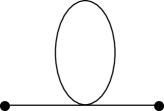
Figure 1: One-loop diagram having one four-point interaction vertex for the two-point correlation function.

The end points of the loop are connected to the same four-point vertex. Therefore the factor coming from the integral of this loop becomes $\int d^{3}k\,\mathcal{P}(k)$. Substituting the scale invariant power spectrum into $\mathcal{P}(k)\propto k^{-3}$, we find that the integral is logarithmically divergent in the IR limit like $\int d^{3}k/k^{3}$. As is seen also in this simple example, the IR divergences are typically logarithmic Onemli:2002hr ; Brunier:2004sb ; Prokopec:2007ak ; Sloth:2006az ; Sloth:2006nu ; Seery:2007we ; Seery:2007wf ; Urakawa:2008rb ; Cogollo:2008bi ; Rodriguez:2008hy . To be a little more precise, we also need to care about UV divergences. However, since the fluctuation modes whose wavelength is well below the horizon scale (sub-horizon modes) do not feel the cosmic expansion, they are expected to behave as if in Minkowski spacetime. Namely, the quantum state of sub-horizon modes is approximately given by the one in the adiabatic vacuum. Hence, the sub-horizon modes will not give any time-dependent cumulative contribution to the loop integral after appropriate renormalization. They are therefore irrelevant for the discussions in this paper. Throughout this paper, we neglect the contribution due to sub-horizon modes by introducing the UV cut-off of momentum at around the co-moving horizon scale $aH$ where $a$ is the scale factor and $H$ is the expansion rate of the universe.

As a practical way to make the loop corrections finite, we often introduce the IR cut-off at the co-moving scale corresponding to the Hubble horizon scale at the initial time, $a_{i}H_{i}$ Afshordi:2000nr . This kind of artificial IR cut-off is not fully satisfactory because it leads to the logarithmic amplification of the loop corrections as we push the initial time to the past like

$$(\mbox{Loop integral})\sim\int_{aH>|k|>a_{i}H}d^{3}k\,k^{-3}\propto\log(a/a_{i})~{},$$ (1)

where $a_{i}$ is the scale factor at the initial time and we neglected the time dependence of the Hubble parameter. Due to the non-vanishing IR contribution, the choice of the IR cut-off affects the amplitude of loop corrections. Furthermore, the reason why we select a specific IR cut-off is not clear. This means that, in order to obtain a reliable estimate for the IR corrections, we need to derive a scheme to make the corrections finite from physically reasonable requirements. This is what we wish to discuss in this paper.

To begin with, we point out that the usual gauge invariant perturbation theory cannot describe the fluctuations that we actually observe. This is because we can observe only the fluctuations within the region causally connected to us. To discuss the so-called observable quantities in the framework of the gauge invariant perturbation, in general, it is necessary to fix the gauge in all region of the universe. However, in reality it is impossible for us to make observations imposing the gauge conditions in the region causally disconnected from us. Since we cannot specify the gauge conditions in the causally disconnected region, the gauge invariant variables that we usually consider as observables are undetermined. We need to be careful also in defining what are the observable fluctuations. We usually define the fluctuation by the deviation from the background value which is the spatial average over the whole universe. However, since we can observe only a finite volume of the universe, the fluctuations evaluated in such a way are inevitably influenced by the information contained in the unobservable region. In particular, in the chaotic inflation the longer wavelength mode has the larger amplitude of fluctuation Lidsey:1995np ; Bassett:2005xm ; Lyth:2007qh ; Linde:2007fr , and therefore the value averaged over the whole universe is not even well-defined. In general, the deviation from the global average is much larger than the deviation from the local average, which leads to the over-estimation of the fluctuations due to the contribution from long wavelength fluctuations.

In this paper, we show that, taking an appropriate gauge, we can compute the evolution of fluctuations which better correspond to what we actually observe. It is often the case to adapt the flat gauge or the comoving gauge in computing nonlinear quantum effects. Those are thought to be a way of complete gauge fixing. However, in § II, we will explain that, even if we impose such gauge conditions in the observable finite region, the gauge conditions are not completely fixed. To remove the residual gauge degrees of freedom, we impose further gauge conditions. In doing so, we require also the gauge fixing conditions not to be affected by the influence from the causally disconnected region. The violation of causality due to careless choice of variables, even if it is superficial such as pure gauge contributions, can lead to divergences in computation. In § III, we prove that IR corrections no longer diverge in the single field model, once we adopt an appropriate choice of variables with appropriate gauge conditions. We also show that the amplitude of perturbation does not grow secularly even if we send the initial time to the distant past unless very higher order perturbations are considered. In § IV, we summarize our statement.

II A prescription to solve IR problem

II.1 Setup of the problem

We first define the setup that we study in this paper. We consider the single field inflation model with the conventional kinetic term. The total action is given by

$$S=\frac{1}{2}\int\sqrt{-g}~{}[M_{\rm pl}^{2}R-g^{\mu\nu}\Phi_{,\mu}\Phi_{,\nu}-2U(\Phi)]d^{4}x~{}.$$ (2)

where $M_{\rm pl}$ is the Planck mass. We perform the following change of variables

$$\phi\equiv\Phi/M_{\rm pl},\quad V(\phi)\equiv U(\Phi)/M_{\rm pl}^{2},$$ (3)

to factorize $M_{\rm pl}^{2}$ from the action as

$$S=\frac{M_{\rm pl}^{2}}{2}\int\sqrt{-g}~{}[R-g^{\mu\nu}\phi_{,\mu}\phi_{,\nu}-2V(\phi)]d^{4}x~{}.$$ (4)

Hereafter we work with this rescaled non-dimensional field $\phi$. For simplicity, we assume that $V(\phi)$ and all of its higher order derivatives are at most $O(H^{2})$, where $H$ is the Hubble parameter. This condition is satisfied in slow roll inflation. Since the Planck mass is completely factored out, the equations of motion do not depend on it. The Planck mass appears only in the amplitude of quantum fluctuation. Namely, the typical amplitude of fluctuation of $\Phi$ is $H$, and hence that of $\phi$ is $H/M_{\rm pl}$.

In order to discuss the nonlinearity, it is convenient to use the ADM formalism, where the line element is expressed in terms of the lapse function $N$, the shift vector $N^{a}$, and the purely spatial metric $h_{ab}$:

$$ds^{2}=-N^{2}dt^{2}+h_{ab}(dx^{a}+N^{a}dt)(dx^{b}+N^{b}dt)~{}.$$ (5)

Substituting this metric form, we can denote the action as

$$S \!\!= \!\!\frac{M_{\rm pl}^{2}}{2}\int\sqrt{h}\Bigl{[}N~{}^{(3)}R-2NV(\phi)+\frac{1}{N}(E_{ab}E^{ab}-E^{2})$$ (6)

$$\hskip 14.22636pt+~{}\frac{1}{N}(\dot{\phi}-N^{a}\partial_{a}\phi)^{2}-Nh^{ab}\partial_{a}\phi\partial_{b}\phi\Bigr{]}d^{4}x~{},$$

where

$$E_{ab}=\frac{1}{2}\{\dot{h}_{ab}-D_{a}N_{b}-D_{b}N_{a}\}~{},$$ (7)

$$E=h^{ab}E_{ab}~{}.$$ (8)

In the ADM formalism, we can obtain the constraint equations easily by varying the action with respect to $N$ and $N^{a}$, which play the role of Lagrange multipliers. We obtain the Hamiltonian constraint equation and the momentum constraint equations as

$${}^{(3)}R-2V-N^{-2}(E^{ab}E_{ab}-E^{2})$$ (9)

$$\qquad-~{}N^{-2}(\dot{\phi}-N^{a}\partial_{a}\phi)^{2}-h^{ab}\partial_{a}\phi\partial_{b}\phi=0~{},$$ (10)

$$D_{a}[N^{-1}(E^{a}_{~{}b}-\delta^{a}_{~{}b}E)]-N^{-1}\partial_{b}\phi~{}(\dot{\phi}-N^{a}\partial_{a}\phi)=0~{}.$$

Hereafter, neglecting the vector perturbation, we denote the shift vector as $N_{a}=\partial_{a}\chi$. In this paper we work in the flat gauge, defined by

$$h_{ab}=e^{2\rho}\delta_{ab}~{},$$ (12)

where $a\equiv e^{\rho}$ is the background scale factor. Here we have also neglected the tensor perturbation, focusing only on the scalar perturbation, in which the IR divergence of our interest arises Boyanovsky:2005px ; Urakawa:2008rb .

In this gauge, using $N$, $\chi$ and the fluctuation of the scalar field $\varphi$, the total action is written as

$$S \!= \!\frac{M_{\rm pl}^{2}}{2}\int dtd^{3}\!{\bm{x}}\,e^{3\rho}\Bigl{[}~{}-2N~{}\displaystyle\sum_{n=0}\frac{1}{n!}V^{(n)}(\phi)\varphi^{n}$$

$$~{}~{}+N^{-1}\{-6\dot{\rho}^{2}+4\dot{\rho}~{}\triangle\chi$$

$$\hskip 71.13188pt+(\nabla^{a}\nabla^{b}\chi\nabla_{a}\nabla_{b}\chi-(\triangle\chi)^{2})\}$$

$$~{}~{}+N^{-1}(\dot{\phi}+\dot{\varphi}-\nabla^{a}\chi\nabla_{a}\varphi)^{2}-N(\nabla\varphi)^{2}\Bigr{]}~{},$$

and two constraint equations are

$$2N^{2}\displaystyle\sum_{n=0}\frac{1}{n!}(\partial_{\phi}^{n}V(\phi))\varphi^{n}-6\dot{\rho}^{2}$$

$$~{}~{}+4\dot{\rho}\triangle\chi+\{\nabla^{a}\nabla^{b}\chi\nabla_{a}\nabla_{b}\chi-(\triangle\chi)^{2}\}$$

$$~{}~{}+(\dot{\phi}+\dot{\varphi}-\nabla^{a}\chi\nabla_{a}\varphi)^{2}+N^{2}(\nabla\varphi)^{2}=0,$$

(14)

$$(\nabla_{a}N)\{2\dot{\rho}\delta^{a}_{~{}b}+(\nabla^{a}\nabla_{b}\chi-\delta^{a}_{~{}b}\triangle\chi)\}$$

$$~{}~{}-(\nabla_{b}\varphi)N~{}(\dot{\phi}+\dot{\varphi}-\nabla^{a}\chi\nabla_{a}\varphi)=0~{},$$

where

$$\nabla_{a}\equiv e^{-\rho}\partial_{a}~{},$$

represents the three dimensional partial differentiation with respect to the proper length coordinates $e^{\rho}{\bm{x}}$ and

$$\triangle\equiv\delta^{ab}\nabla_{a}\nabla_{b}~{}.$$

Spatial indices, $a,b,\cdots$, are raised by $\delta^{ab}$. This notation, which respects the proper distance, is convenient for the later discussions because it eliminates all the complicated scale factor dependences from the action.

The background quantities $\rho$ and $\phi$ satisfy

$$3\dot{\rho}^{2}=\frac{1}{2}\dot{\phi}^{2}+V(\phi)~{},$$

$$\ddot{\phi}+3\dot{\rho}~{}\dot{\phi}+V_{\phi}=0~{},$$

$$\ddot{\rho}=-\frac{1}{2}\dot{\phi}^{2}~{},$$ (16)

where $V_{\phi}\equiv\partial_{\phi}V(\phi)$. Expanding $N$, $\chi$ and $\varphi$ as

$$N = 1+\delta N_{1}+\frac{1}{2}\delta N_{2}+\cdots,$$ (17)

$$\chi = \chi_{1}+\frac{1}{2}\chi_{2}+\cdots~{},$$ (18)

$$\varphi = \varphi_{1}+\frac{1}{2}\varphi_{2}+\cdots~{},$$ (19)

we find that the first order constraint equations are written as

$$V_{\phi}\varphi_{1}+2V\delta N_{1}+2\dot{\rho}\triangle\chi_{1}+\dot{\phi}~{}\dot{\varphi}_{1}=0~{},$$ (20)

$$\nabla_{a}(2\dot{\rho}~{}\delta N_{1}-\dot{\phi}~{}\varphi_{1})=0~{},$$ (21)

and the second order ones as

$$V_{\phi}\varphi_{2}+2V\delta N_{2}+2\dot{\rho}\triangle\chi_{2}+\dot{\phi}~{}\dot{\varphi}_{2}$$ (22)

$$~{}~{}~{}+V_{\phi\phi}\varphi^{2}+2V\delta N_{1}^{2}+4V_{\phi}\delta N_{1}\varphi_{1}$$ (23)

$$~{}~{}~{}+2\dot{\rho}\triangle\chi_{2}+~{}\nabla^{a}\nabla^{b}\chi_{1}\nabla_{a}\nabla_{b}\chi_{1}-(\triangle\chi_{1})^{2}$$ (24)

$$~{}~{}~{}-2\dot{\phi}e^{-2\rho}\nabla^{a}\chi_{1}\nabla_{a}\varphi_{1}+\dot{\varphi}_{1}^{2}+(\nabla\varphi_{1})^{2}=0~{},$$ (25)

$$\nabla_{a}(2\dot{\rho}~{}\delta N_{2}-\dot{\phi}~{}\varphi_{2})$$ (26)

$$~{}~{}~{}+2(\nabla_{b}\delta N_{1})(\nabla^{b}\nabla_{a}\chi_{1}-\delta^{b}_{~{}a}\triangle\chi_{1})$$ (27)

$$~{}~{}~{}-2\nabla_{a}\varphi_{1}(\dot{\phi}~{}\delta N_{1}+\dot{\varphi}_{1})=0~{}.$$ (28)

Taking the variation of the action with respect to $\varphi$, we can derive the equation of motion for $\varphi$, which includes the Lagrange multipliers $\delta N$ and $\chi$. For example, from the third order action, we can derive the equation of motion with quadratic interaction terms as follows,

$$\ddot{\varphi}+3\dot{\rho}\dot{\varphi}-\triangle\varphi+V_{\phi\phi}\varphi-\dot{\phi}\triangle\chi+\delta NV_{\phi}-3\dot{\rho}\,\dot{\phi}\delta N-\partial_{t}(\delta N\dot{\phi})$$

$$\hskip 14.22636pt+\frac{1}{2}V_{\phi\phi\phi}\varphi^{2}-\nabla_{a}(\dot{\varphi}-\dot{\phi}\delta N)\nabla^{a}\chi-(\dot{\varphi}-\dot{\phi}\delta N)\triangle\chi-\dot{\rho}\nabla^{a}\chi\nabla_{a}\varphi-\partial_{t}(\nabla^{a}\chi\nabla_{a}\varphi)$$

$$\hskip 14.22636pt-3\dot{\rho}\,\dot{\varphi}\,\delta N-\partial_{t}(\delta N\dot{\varphi})-\nabla_{a}(\delta N\nabla^{a}\varphi)+V_{\phi\phi}\,\varphi\,\delta N+3\dot{\rho}\,\dot{\phi}\,\delta N^{2}+\partial_{t}(\dot{\phi}\,\delta N^{2})=0~{}.$$ (29)

Solving the constraint equations for the lapse function and shift vector at each order, we can express $\delta N$ and $\chi$ as functions of $\varphi$. Substituting these expressions into the original action (LABEL:action_in_flat), we obtain the reduced action in the flat gauge written solely in terms of the dynamical degrees of freedom, $\varphi$.

II.2 Tree-shaped graphs

In this subsection, as a preparation for computing $n$-point functions of $\varphi(x)$, we consider an expansion of the Heisenberg field $\varphi(x)$ in terms of the interaction picture field $\varphi_{I}(x)$. When we compute $n$-point functions for a given initial state, we often use the closed time path formalism Chou:1984es ; Jordan:1986ug ; Calzetta:1986ey , in which $n$-point functions are perturbatively expanded by using the four different types of Green functions: the Wightman function $G^{+}(x,x^{\prime})$, the Feynman propagator $G_{F}(x,x^{\prime})$ and their complex conjugations $G^{-}(x,x^{\prime})$ and $G_{D}(x,x^{\prime})$. Here we shall adopt a different approach in which we take the full advantage of using the retarded (or advanced) Green function. In contrast to the above four Green functions, the retarded Green function

$$G_{R}(x,x^{\prime})=i\theta(t-t^{\prime})M^{2}_{\rm pl}\{G^{+}(x,x^{\prime})-G^{-}(x,x^{\prime})\}~{},$$ (30)

(31)

is non-vanishing only when $x$ is in the causal future of $x^{\prime}$. In fact, when these two points are mutually space-like, the two field operators $\varphi(x)$ and $\varphi(x^{\prime})$ commute with each other, which leads to $G^{+}(x,x^{\prime})=G^{-}(x,x^{\prime})$. Since the retarded Green function $G_{R}(x,x^{\prime})$ has a finite non-vanishing support for fixed $t$ and $t^{\prime}$, its three dimensional Fourier transform becomes regular in the IR limit, while the other Green functions behave like $k^{-3}$. (This IR behaviour leads to the scale invariant power spectrum, $P(k)\propto 1/k^{3}$. We will discuss these issues in more detail later.) Hence, in order to prove the IR regularity in loop corrections to $n$-point functions, it is convenient to use $G_{R}(x,x^{\prime})$ as much as possible.

Let us denote the equation of motion for $\varphi$ schematically as

$${\cal L}\varphi=-\Gamma[\varphi]~{},$$ (32)

where ${\cal L}$ is a second order differential operator corresponding to the linearized equation for $\varphi$ (Eq. (49)) and $\Gamma$ stands for all the nonlinear interaction terms. We stress that this equation of motion does not depend on $M_{pl}$ as anticipated. Using the retarded Green function $G_{R}(x,x^{\prime})$ that satisfies

$${\cal L}G_{R}(x,x^{\prime})=-a^{-3}\delta^{4}(x-x^{\prime})~{},$$ (33)

we can solve Eq. (32) formally as

$$\varphi(x)=\varphi_{I}(x)+\int d^{4}\!x^{\prime}\,G_{R}(x,x^{\prime})a^{3}(t^{\prime})\Gamma[\varphi](x^{\prime}).$$ (34)

Here the factor $a^{3}$ originates from the background value of $\sqrt{-g}$. Substituting this expression for $\varphi(x)$ iteratively into $\Gamma[\varphi]$ on the r.h.s., we obtain the Heisenberg field $\varphi(x)$ expanded in terms of $\varphi_{I}(x)$ to any order using the retarded Green function $G_{R}(x,x^{\prime})$. A diagrammatic illustration as given in Fig. 2 will be useful. In Fig. 2 we showed the procedure of expanding the Heisenberg operator when only a simple three-point interaction is present, i.e. $\Gamma[\varphi]=\frac{\lambda}{2!}\varphi^{2}$. Here, we represent the Heisenberg field, the interaction picture field, and the retarded Green function by a thick line, a thin line and a thin line associated with the index “$R$”, respectively. Now it will be easy to understand that the Heisenberg field can be expressed by a summation of tree-shaped graphs of this kind not only for this specific case, but also for any polynomial interaction. Let us summarize the structure of tree-shaped graphs. Looking at a tree-shaped graph from left to right, it starts with a retarded Green function except for the first trivial graph that does not contain any vertex. All the retarded Green functions $G_{R}(x,x^{\prime})$ are followed by two or more $\varphi_{I}(x^{\prime})$ or $G_{R}(x^{\prime},x^{\prime\prime})$ with some integro-differential operators. All the interaction picture fields $\varphi_{I}(x)$ are located at the right most ends of the graphs.

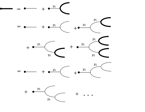
Figure 2: Diagrammatic expression for the Heisenberg field expanded in terms of the interaction picture fields when only the three point interaction vertex is present. Here the Heisenberg field, the interaction picture field, and the retarded Green function are represented by a thick line, a thin line and a thin line with the index “$R$”, respectively.

When we compute the expectation value for $n$-point functions of the Heisenberg field, the interaction picture fields $\varphi_{I}$ that appear at the right ends of tree-shaped graphs are contracted with each other to make pairs. Then, when we evaluate the expectation value, the pairs of $\varphi_{I}$ are replaced with Wightman functions, $G^{+}(x,x^{\prime})$ or $G^{-}(x,x^{\prime})(=G^{+}(x^{\prime},x))$. As these propagators are IR singular ($\propto 1/k^{3}$) in contrast to $G_{R}(x,x^{\prime})$, they are the possible origin of IR divergences in momentum integrations.

II.3 Gauge degree of freedom in flat gauge

We consider the time evolution for the period $[t_{i},~{}t_{f}]$, where $t_{f}$ represents the final time at which we evaluate the field fluctuations. In this paper we assume that the universe is still inflating at $t=t_{f}$. Reflecting the fact that our observable region is bounded, we evaluate only the fluctuations within a finite region ${\cal O}_{t_{f}}$, and we denote the causal past of this region ${\cal O}_{t_{f}}$ by ${\cal O}$. To exclude the effect from the unobservable part of the universe, the evolution of $\varphi$ in ${\cal O}$ should be determined without any knowledge about the region outside ${\cal O}$. If $\Gamma[\varphi]$ were written in terms of local functions of $\varphi$, Eq. (32) would determine the Heisenberg field $\varphi(x)$ for $x\in{\cal O}_{t_{f}}$ solely written in terms of the interaction picture fields $\varphi_{I}(x^{\prime})$ with $x^{\prime}\in{\cal O}$. However, we also need to solve equations of elliptic-type such as Eqs. (20), (21), (25), and (28). The solutions of these constraint equations, which determine the lapse function and the shift vector, depend on the boundary conditions when a finite volume is assumed. Irrespective of the distance to the boundary, the boundary conditions immediately affect the solution owing to the non-hyperbolic nature of the equations.

In the linear order, these extra degrees of freedom appears as an arbitrary time-dependent integration constant. Indeed, we can solve the first order momentum constraint equation (21) as

$$\delta{N}_{1}(x) = f_{1}(t)+\frac{\dot{\phi}}{2\dot{\rho}}{\varphi}_{1}(x)~{},$$ (35)

where an arbitrary function $f_{1}(t)$ was introduced as an integration constant. Substituting this into the lowest order Hamiltonian constraint (20), we can solve it for $\chi_{1}$ to obtain

$${\chi}_{1}(x)=-\frac{\dot{\phi}^{2}}{2\dot{\rho}^{2}}\triangle^{-1}\partial_{t}\Bigl{(}\frac{\dot{\rho}}{\dot{\phi}}{\varphi}_{1}\Bigr{)}-\frac{V}{6\dot{\rho}}f_{1}(t)r^{2},$$ (36)

where $r$ is the proper spatial distance from the center defined by

$$r^{2}=e^{2\rho}x_{a}x^{a}.$$

Since the last term in Eq.(36) proportional to $r^{2}$ cannot be expanded in terms of the spatial harmonics ($\approx e^{i\hbox{\boldmath{\scriptsize$kx$}}}$), we do not have this residual gauge degree of freedom in the standard cosmological perturbation scheme. Here, we do not care about the region outside ${\cal O}$. Then, the solution of Eq. (20) restricted to the region ${\cal O}$ is not uniquely determined. Although we could have added more arbitrary harmonic functions (homogeneous solutions of the Poisson equation) with time-dependent coefficients to the above solution for $\chi_{1}$, we neglected them for simplicity.

The degree of freedom $f_{1}(t)$ introduced above corresponds to scale transformation:

$$x^{a}~{}\longrightarrow~{}~{}\tilde{x}^{a}=e^{\dot{\rho}\alpha(t)}x^{a}~{}.$$ (37)

Such a scale transformation is compatible with the perturbative expansion only when our interest is concentrated on a finite region of spacetime. Once we consider an infinite volume, this transformation does not remain to be a small change of coordinates irrespective of the amplitude of $\alpha(t)$. Simultaneously, we apply the time coordinate transformation $t~{}\rightarrow~{}\tilde{t}=t-\alpha(t)$. Under this transformation, in the linear order, the spatial metric components are transformed to

$$\tilde{h}_{ab}(\tilde{x}) = e^{-2\dot{\rho}\alpha(t)}\,h_{ab}(x)$$ (38)

$$= e^{-2\dot{\rho}\alpha(t)}e^{2\rho(\tilde{t}+\alpha(t))}\,\delta_{ab}(x)$$ (39)

$$= e^{2\rho(\tilde{t})}\delta_{ab}~{}.$$ (40)

Thus, we find that this scale transformation keeps the flat gauge conditions that we imposed on the spatial metric (12) unchanged, and therefore it is in fact a residual gauge degree of freedom.

Under the same coordinate transformation with the identification

$$f_{1}=\dot{\alpha}-{\dot{\phi}^{2}\over 2\dot{\rho}}\alpha~{},$$ (41)

we can easily confirm that the first order lapse function and the shift vector transform as given in Eqs.(35) and (36). Here we have explained only for the first order lapse function and the shift vector, the corresponding degree of freedom also exists in the higher order. In this paper we focus on the flat gauge, but a similar discussion applies for the comoving gauge, too.

II.4 Iteration scheme and local gauge conditions

As is mentioned in § I, our final goal is to define finite observable quantities in place of the naively divergent quantum correlation functions. We should note that in general, we cannot discuss observables in the gauge invariant manner by fixing the gauge completely over the whole universe. In this subsection, we show that imposing the boundary conditions unaffected by the information in the outside region, we can shut off the influence from the unobservable region of the universe. (We refer to such a gauge as a local gauge, in which the causality is maintained also for the evolution of quantum Heisenberg field operators.) Once we choose the local gauge, we need not to care about the evolution outside the observable region as well as the gauge conditions there.

Keeping the flat gauge conditions, we impose an additional local gauge condition:

$$\hat{W}_{t}\tilde{\varphi}(t)\equiv\frac{1}{L_{t}^{3}}\int d^{3}\bm{x}~{}W_{t}(\bm{x})~{}\tilde{\varphi}(t,~{}\bm{x})=0~{},$$ (42)

by using the degree of freedom $f_{1}(t)$ introduced in the preceding subsection and its higher order extension, where $W_{t}(\bm{x})$ is a window function, which is unity in the finite region ${\cal O}_{t}\equiv{\cal O}\cap\Sigma_{t}$ with a rapidly vanishing halo in the surrounding region, where $\Sigma_{t}$ means a $t=$const. hypersurface corresponding to the time $t$. For definiteness, we introduce ${\cal O}^{\prime}_{t_{f}}\supset{\cal O}_{t_{f}}$ and define ${\cal O}^{\prime}$ as the causal past of ${\cal O}^{\prime}_{t_{f}}$. We require $W_{t}(\bm{x})$ to vanish in the region outside ${\cal O}^{\prime}$. In addition, $W_{t}(\bm{x})$ is supposed to be a sufficiently smooth function so that an artificial UV contribution is not induced by a sharp cutoff. $L_{t}$, an approximate radius of the region ${\cal O}_{t}$, is defined such that the normalization condition

$$\hat{W}_{t}1=1~{},$$

is satisfied.

Roughly speaking, $L_{t}$ follows the radial null geodesic equation. Hence, we have

$$L_{t}\approx\int{dt\over a(t)}\approx L_{t_{f}}+{1\over a(t)H(t)}~{}.$$ (43)

For $t\gtrsim t_{c}$, we have $L_{t}\approx L_{t_{f}}$, where $t_{c}$ is defined by $a(t_{c})H(t_{c})L_{t_{f}}=1$. While, for $t\lesssim t_{c}$, $L_{t}$ agrees with the comoving horizon radius at that time. (See Fig. 4.)

By construction, $\tilde{\varphi}$ represents the deviation from the local average value in ${\cal O}_{t}$. We associated “$~{}\tilde{}~{}$” with the variables in this particular gauge, in order to clearly distinguish them from the variables for which the above additional gauge condition is not imposed. The difference between the variables with and without “$~{}\tilde{}~{}$” is only in the boundary conditions. Hence, they obey the same differential equations, (21)-(29).

Now we give a prescription to fix the arbitrary function $f_{1}(t)$ in Eqs. (35) and (36) as well as its higher order counterpart $f_{n}(t)$ ($n=2,3,4,\cdots$) to satisfy the gauge condition (42). For this purpose, we need to obtain a formal solution for $\tilde{\varphi}$. First, we consider the equations to fix the lapse functions. The higher order lapse functions are determined by the momentum constraint given in the form

$$\nabla_{a}\left(\delta\tilde{N}_{n}-{\dot{\phi}\over 2\dot{\rho}}\varphi_{n}\right)=\Xi^{(n)}_{a},\quad(n=1,2,3,\cdots),~{}$$ (44)

where the r.h.s. is a three vector at $n$-th order nonlinear terms expressed in terms of the lower order lapse functions, shift vectors, and $\tilde{\varphi}$. These equations do not have a solution in general since there are three equations with one variable. This situation happens because we have neglected the vector perturbation. Hence, we consider only the scalar part of these equations, i.e. its divergence. This prescription is consistent with our neglecting the vector perturbation. The scalar part of Eq.(2.32) is formally solved as

$$\delta\tilde{N}_{n}=\delta\breve{N}_{n}+f_{n},$$ (45)

with

$$\delta\breve{N}_{n}={\dot{\phi}\over 2\dot{\rho}}\varphi_{n}+\triangle^{-1}\nabla^{a}\Xi^{(n)}_{a}.$$

The operation $\triangle^{-1}$ in Eq. (36) is also to be defined so as to be completely determined by the local information in the neighborhood of ${\cal O}_{t}$. We therefore define $\triangle^{-1}$ by

$$\triangle^{-1}F(x)=-\frac{1}{4\pi}\int\frac{W_{t}(e^{-\rho}{\bm{Y}})d^{3}{\bm{Y}}}{|{\bm{X}}-{\bm{Y}}|}F(t,e^{-\rho}{\bm{Y}})~{}.$$ (46)

where we have used the proper length coordinates ${\bm{X}}\equiv e^{\rho}{\bm{x}}$ . Similarly, the higher order shift vectors satisfy the Hamiltonian constraint in the form

$$\triangle\tilde{\chi}_{n} = -{1\over 2}\!\left({\dot{\phi}\over\dot{\rho}}\right)^{2}\partial_{t}\left({\dot{\rho}\over\dot{\phi}}\varphi_{n}\right)$$

$$\qquad\qquad-{V\over\dot{\rho}}\left(f_{n}+\triangle^{-1}\nabla^{a}\Xi^{(n)}_{a}\right)+C_{n},$$

where $C_{n}$ on the r.h.s. is a function expressed in terms of the lower order lapse functions, shift vector and $\tilde{\varphi}$. A formal solution for $\tilde{\chi}_{n}$ is given by

$$\tilde{\chi}_{n} \!\!= \!\!\breve{\chi}_{n}-{r^{2}V\over 6\dot{\rho}}f_{n}~{},$$ (47)

with

$$\breve{\chi}_{n} = -\triangle^{-1}\Biggl{(}{1\over 2}\!\left({\dot{\phi}\over\dot{\rho}}\right)^{2}\partial_{t}\left({\dot{\rho}\over\dot{\phi}}\varphi_{n}\right)$$

$$\qquad\qquad\qquad\qquad+{V\over\dot{\rho}}\triangle^{-1}\left(\nabla^{a}\Xi^{(n)}_{a}\right)+C_{n}\Biggr{)}~{}.$$

Next, we consider the equation of motion for $\tilde{\varphi}$, which is Eq. (29) with all perturbation variables replaced to the ones with “$~{}\tilde{}~{}$”. Substituting the expressions for the lapse function (45) and the shift vector (47) into the equation of motion for $\tilde{\varphi}$ truncated at the $n$-th order, we obtain an equation

$${\cal L}\tilde{\varphi}_{n}-\dot{\phi}\dot{f}_{n}+\left({V\dot{\phi}\over\dot{\rho}}+2V_{\phi}\right)f_{n}=-\Gamma_{n},$$ (48)

where

$${\cal L}\equiv\partial^{2}_{t}+3\dot{\rho}\,\partial_{t}-\triangle+\left(V_{\phi\phi}-e^{-3\rho}\dot{A}\right).$$ (49)

with

$$A(t)\equiv e^{3\rho}\dot{\phi}^{2}/\dot{\rho}~{},$$

and $\Gamma_{n}$ on the r.h.s. of Eq. (48) represents all the remaining nonlinear terms expressed in terms of lower order terms in $f(t)$ and $\tilde{\varphi}$.

The equation for $\tilde{\varphi}_{n}$ is obtained by eliminating $f_{n}$ from Eq. (48) by operating $\hat{\bar{W}}_{t}\equiv 1-\hat{W}_{t}$ as

$$\hat{\bar{W}}_{t}\,{\cal L}\tilde{\varphi}_{n}=-\hat{\bar{W}}_{t}\,\Gamma_{n}[\tilde{\varphi}]~{}.$$ (50)

This equation alone is not sufficient to determine $\tilde{\varphi}_{n}$ because its homogeneous part is projected out. The homogeneous part of $\tilde{\varphi}_{n}$ is determined by the gauge condition $\hat{W}_{t}\,\tilde{\varphi}_{n}=0$. Practically, $\tilde{\varphi}_{n}(x)$ is obtained by

$$\tilde{\varphi}_{n}(x)\equiv\hat{\bar{W}}_{t}\,\breve{\varphi}_{n}(x)~{},$$ (51)

where $\breve{\varphi}_{n}$ satisfies

$${\cal L}\breve{\varphi}_{n}(x)=-W_{t}({\bm{x}})\Gamma_{n}[\tilde{\varphi}]~{}.$$ (52)

Here, for later convenience, we have inserted a window function $W_{t}({\bm{x}})$ on the r.h.s. of Eq. (52), although it is possible to get the same conclusion without introducing this factor. As an effect of this inserted factor, thus obtained $\tilde{\varphi}_{n}(x)$ satisfies the field equation (48) only within the region ${\cal O}$.

We found a way to obtain $\tilde{\varphi}_{n}$ before we know $f_{n}$. Now we discuss how to fix $f_{n}$. Operating $\hat{W}_{t}\equiv\frac{1}{L_{t}^{3}}\int d^{3}{\bm{x}}W_{t}({\bm{x}})$ on Eq. (49), we obtain

$$\dot{\phi}\dot{f}_{n}-\left({V\dot{\phi}\over\dot{\rho}}+2V_{\phi}\right)f_{n}=\hat{W}_{t}(\Gamma_{n}+{\cal L}\tilde{\varphi}_{n}),$$ (53)

Using $A(t)$, which satisfies the corresponding homogeneous equation

$$\frac{\dot{A}}{A}=-\frac{V}{\dot{\rho}}-2{V_{\phi}\over\dot{\phi}}=3\dot{\rho}-{\ddot{\rho}\over\dot{\rho}}+2{\ddot{\phi}\over\dot{\phi}}~{},$$ (54)

we can solve Eq. (53) for $f_{n}$ as

$$f_{n}(t)=\frac{1}{A(t)}\int^{t}dt^{\prime}~{}\frac{A(t^{\prime})}{\dot{\phi}(t^{\prime})}\hat{W}_{t^{\prime}}(\Gamma_{n}+{\cal L}\tilde{\varphi}_{n}).$$ (55)

Here we note that the r.h.s. is completely written in terms of the lower order perturbation variables and $\tilde{\varphi}_{n}$, both of which are already given.

From the above discussions we find that the lapse function, the shift vector and $\tilde{\varphi}$ can be solved iteratively. Therefore all the higher order terms can be written in terms of $\tilde{\varphi}_{1}(x)=\hat{\bar{W}}_{t}\varphi_{I}(x)$ with $x\in{\cal O}^{\prime}_{t_{i}}$. In this sense, our prescription to find a solution of Heisenberg equations within ${\cal O}$ guarantees approximate causality, avoiding influence from the outside of ${\cal O}^{\prime}$. We summarize our iteration scheme in Fig. 3.

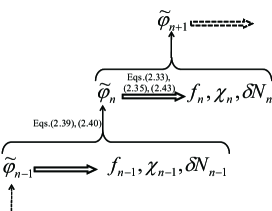
Figure 3: Summary of the iteration scheme to obtain higher order perturbation $\tilde{\varphi}_{n}$.

To summarize, we defined observable perturbations, which are not affected by the information in the region outside ${\cal O}^{\prime}$, by imposing an additional local gauge condition. Imposing appropriate boundary conditions in solving elliptic-type equations that determine the lapse function and shift vector, we have shown that the local gauge condition that we require can be consistently imposed and the influence from the causally disconnected region is completely shut off in this gauge, in contrast to the traditional flat gauge.

II.5 Quantization

Even if we consider the perturbations in the local flat gauge, to quantize the fluctuation and to specify the initial state, we have to start with the ordinary flat gauge. This is because we need to give a complete set of mode functions on a Cauchy surface to specify the initial vacuum state and to constitute the Fock space. After specifying the initial state, we transform the perturbation variables into the local flat gauge, in which the causality is maintained .

Using a set of mode functions $\{\phi_{\hbox{\boldmath{\scriptsize$k$}}}(x)\equiv u_{k}(t)e^{i\hbox{\boldmath{\scriptsize$kx$}}}\}$, which satisfy the linear perturbation equation

$$0 = e^{-i{\hbox{\boldmath{\scriptsize$k$}}}\cdot{\hbox{\boldmath{\scriptsize$x$}}}}{\cal L}\phi_{\hbox{\boldmath{\scriptsize$k$}}}$$ (56)

$$= \left[\partial^{2}_{t}+3\dot{\rho}\partial_{t}+e^{-2\rho}k^{2}+\left(V_{\phi\phi}-{\dot{A}\over e^{3\rho}}\right)\right]u_{\hbox{\boldmath{\scriptsize$k$}}}(t)~{},$$ (57)

we expand the globally defined interaction picture field as

$$\varphi_{I}(x)=\int\frac{d^{3}{\bm{k}}}{(2\pi)^{3/2}}~{}\left\{{u_{k}(t)\over M_{\rm pl}}e^{i{\hbox{\boldmath{\scriptsize$k$}}}\cdot{\hbox{\boldmath{\scriptsize$x$}}}}a_{\hbox{\boldmath{\scriptsize$k$}}}+\mbox{h.c.}\right\}~{}.$$ (59)

Here the creation and annihilation operators, $a_{\hbox{\boldmath{\scriptsize$k$}}}^{\dagger}$ and $a_{\hbox{\boldmath{\scriptsize$k$}}}$, satisfy the commutation relation

$$\left[a_{\lower 2.0pt\hbox{$\hbox{\boldmath{\scriptsize$k$}}$}},a_{{\hbox{\boldmath{\scriptsize$k$}}}^{\prime}}^{\dagger}\right]=\delta^{3}({\bm{k}}-{\bm{k}}^{\prime}).$$

The mode functions are normalized by

$$u_{k}(t)\dot{u}^{*}_{k}(t)-\dot{u}_{k}(t)u^{*}_{k}(t)={i\over a^{3}(t)}~{}.$$ (60)

The initial vacuum state $|0\rangle$ is annihilated by the operation of any annihilation operator:

$$\!a_{\hbox{\boldmath{\scriptsize$k$}}}|0\rangle=0\hskip 28.45274pt\mbox{for}~{}~{}^{\forall}{\bm{k}}~{}.$$

We assume that the initial vacuum state is not so different from the adiabatic vacuum state at the initial time, especially for the long wavelength modes. On the initial surface, the Heisenberg operator corresponding to the scalar field fluctuation in the local flat gauge is related to that in the ordinary flat gauge as $\tilde{\varphi}_{1}(x)=\hat{\bar{W}}_{t}\varphi_{1}(x)$.

III IR regularity

In this section, we show that $n$-point functions for $\tilde{\varphi}$ are IR regular for the most of inflation models. In § III.1 we study the behavior of the mode function, especially focusing on the long wavelength limit. We show that the Wightman function is singular in the long wavelength limit like $1/k^{3}$, while the retarded Green function is completely regular. In § III.2 we will show that $n$-point functions calculated following our prescription are free from IR divergences in momentum integration when we do not care about secular growth of the amplitude of perturbation, which will be discussed in § III.3. We will show that the secular growth does not occur unless very higher order perturbation is concerned. Secular growth means the increase of the amplitude of fluctuation in proportion to some power of the e-folding number $N$ in the slow-roll limit. Here, as we discuss more general setup in which $H(t)$ monotonically decreases, $t$ is bounded by the condition $H(t)<H_{i}\ll M_{\rm pl}$. Namely, the initial time is never sent to the infinite past where quantum gravity effects cannot be neglected. Therefore the $e$-holding number $N$ in our setup is not infinitely long. In this sense, there arise no divergences from the time integration. Instead, our main concern is the dependence of the final result on the initial time $t_{i}$.

III.1 IR limit of mode functions and retarded Green function

In this subsection we first discuss generic behavior of mode functions in the long wavelength limit. Using that general notion, we discuss the asymptotic behavior of the retarded Green function $G_{R}(x,x^{\prime})$ in the IR limit.

To obtain the mode functions, $v_{k}\equiv-{\dot{\rho}\over\dot{\phi}}u_{k}$ and the conformal time coordinate $\eta\equiv\int dt/a$ are used. In terms of $v_{k}$, Eq.(LABEL:modeequ) becomes

$$v_{k}^{\prime\prime}(\eta)+2\frac{z^{\prime}}{z}v_{k}^{\prime}(\eta)+k^{2}v_{k}(\eta)=0~{},$$ (61)

where $~{}{}^{\prime}~{}$ denotes a differentiation with respect to $\eta$ and $z^{2}\equiv a^{2}(\dot{\phi}/\dot{\rho})^{2}=-2a^{2}\ddot{\rho}/\dot{\rho}^{2}$. The normalization condition of mode functions (60) becomes

$$v_{k}(\eta)v^{*}_{k}{}^{\prime}(\eta)-v^{\prime}_{k}(\eta)v^{*}_{k}(\eta)={i\over z^{2}(\eta)}~{}.$$ (62)

In the long wavelength limit we obtain two independent growing and decaying solutions as

$$v_{k}^{(g)}=1+k^{2}\int^{\eta}\!{d\eta^{\prime}\over z^{2}(\eta^{\prime})}\int^{\eta^{\prime}}\!d\eta^{\prime\prime}z^{2}(\eta^{\prime\prime})+\cdots,$$ (63)

$$v_{k}^{(d)}=-{1\over 2}\int^{\eta}\!{d\eta^{\prime}\over z^{2}(\eta^{\prime})}+\cdots.$$ (64)

Combining these two solutions, we can construct a mode function that satisfies the normalization condition (62) as

$$v_{k}={1\over c(k)}v_{k}^{(g)}+ic^{*}(k)v_{k}^{(d)},$$ (65)

with an arbitrary parameter $c(k)$.

To proceed further, let us consider a simple case in which the scale factor evolves as $H=H_{0}a^{-\epsilon}$, where $\epsilon\equiv-\dot{H}/H^{2}$ is one of the standard slow roll parameters, and we assume that $\epsilon$ is constant. Since the Hubble parameter should decay as $a$ increases, $\epsilon>0$ is understood. As we are interested in the universe in an accelerated expansion phase, $\dot{a}\propto a^{1-\epsilon}$ should grow as $a$ increases. Hence, $\epsilon<1$ is also required. In this case, the original mode function $u_{k}$ is related to $v_{k}$ as $u_{k}=-\sqrt{2\epsilon}v_{k}$. The above two long wavelength solutions (64) are reduced to

$$v_{k}^{(g)}=1+{k^{2}\over 2(1-\epsilon^{2})a^{2}H^{2}}+\cdots,$$ (66)

$$v_{k}^{(d)}=-{1\over 2\epsilon(1+\epsilon)a^{3}H}+\cdots.$$ (67)

At the horizon crossing, where $k\approx aH$, the growing and decaying solutions should contribute to the positive frequency function $v_{k}$ to the same order if the initial quantum state is not very different from the adiabatic vacuum. Assuming that $\epsilon$ is not very close to 1, this requirement determines the order of magnitude of $c(k)$ as

$$c(k)=O\left(\sqrt{\epsilon k^{3}}/H\right).$$ (68)

First of all, from the above estimate of $c(k)$, we find that the leading order term in $u_{k}$ in the long wavelength limit behaves like $\approx H/\sqrt{\epsilon k^{3}}$. Hence, the Wightman function $G^{+}(x,x^{\prime})\equiv\langle\varphi_{I}(x)\varphi_{I}(x^{\prime})\rangle$ and its complex conjugation $G^{-}(x,x^{\prime})$ have IR divergence. In fact, the Fourier transform of the Wightman function is given by

$$\langle\varphi^{I}_{k}(t)\varphi^{I}_{k}(t^{\prime})\rangle=u_{k}(t)u^{*}_{k}(t^{\prime}),$$ (69)

and it is $O(H^{2}/(\epsilon k^{3}))$ in the long wavelength limit.

The amplitude of oscillations of $u_{k}$ changes approximately in proportion to $1/z\propto 1/a$ on sub-horizon scales, where $k\gg aH$. Hence, the amplitude of the positive and negative frequency functions is enhanced for shorter wavelength modes compared with that in the long wavelength limit. However, if such an enhancement causes problematic divergences, such divergences should be attributed to the issue of UV regularization, which is not our main concern in this paper. On the other hand, the long wavelength limit of the decaying solution $v_{k}^{(d)}$, grows faster than $1/a$ as we decrease $a$. Hence, the absolute magnitude of the expression for $v_{k}^{(d)}$ in the long wavelength limit (67) gives an approximate upper bound on the true value of $|v_{k}^{(d)}|$.

In § III.3 we will also use the expression for the retarded Green function $G_{R}(x,x^{\prime})$. Formally, in terms of mode functions, we can give an expression for the retarded Green function as

$$G_{R}(x,~{}x^{\prime})=-i\theta(t-t^{\prime})\int\frac{d^{3}{\bm{k}}}{(2\pi)^{3}}~{}e^{i{\hbox{\boldmath{\scriptsize$k$}}}\cdot({\hbox{\boldmath{\scriptsize$x$}}}-{\hbox{\boldmath{\scriptsize$x$}}}^{\prime})}R_{k}(t,t^{\prime})~{},$$ (70)

(71)

where

$$R_{k}(t,t^{\prime})\equiv u_{k}(t)u^{*}_{k}(t^{\prime})-u^{*}_{k}(t)u_{k}(t^{\prime})~{}.$$ (72)

Substituting the expression (65), we obtain

$$R_{k}(t(\eta),t^{\prime}(\eta^{\prime}))$$ (73)

$$\quad=-2i\epsilon\left(v_{k}^{(g)}(\eta)v_{k}^{(d)}(\eta^{\prime})-v_{k}^{(d)}(\eta)v_{k}^{(g)}(\eta^{\prime})\right).\quad$$ (74)

Then, using the expressions in Eq. (67), we find that $R_{k}$ is regular in $k$ without any singular behavior in the limit $k\to 0$.

III.2 Momentum integration

Now we are ready to discuss the IR regularity of $n$-point functions of $\tilde{\varphi}(x)$. Our discussion is restricted to the case excluding the slow roll limit $\epsilon\to 0$. In this limit, the background scalar field stays constant. Therefore we cannot choose $\hat{W}_{t}\tilde{\varphi}=0$ by a simple change of time coordinate. As a result, a singular behavior appears in Eq. (55). In the following discussion we do not care about the factor $\epsilon$ in the final estimate of the order of magnitude, assuming that $\epsilon$ is not extremely small D

In this subsection we do not consider the secular growth of the amplitude of perturbation due to the integration for a long period of time. Namely, we consider the case that $t_{i}$ is not very distant past from $t_{f}$. Therefore we do not care about the time integration. We defer this issue to the succeeding subsection. Here we just consider the IR divergences originating from the momentum integration. We show that, if we follow the prescription described in § II, the amplitude of perturbation is IR regular without introducing any IR cutoff scale by hand.

As $\tilde{\varphi}(x)$ is composed of $\tilde{\varphi}_{n}~{}(n=1,2,3,\cdots)$, we use the mathematical induction to show the regularity of all $\tilde{\varphi}_{n}$. $\tilde{\varphi}_{n}(x)$ is, by definition, $n$-th order in the interaction picture field $\varphi_{I}$. Formally, we define $C[\tilde{\varphi}_{n}](x;{\bm{p}}_{1},\cdots,{\bm{p}}_{n})$ by expanding $\tilde{\varphi}_{n}(x)$ as

$$\tilde{\varphi}_{n}(x) = \left[\prod_{j=1}^{n}\int{d^{3}\!p_{j}\over(2\pi p_{j})^{3/2}}a_{{\hbox{\boldmath{\scriptsize$p$}}}_{j}}\right]C[\tilde{\varphi}_{n}](x;{\bm{p}}_{1},\cdots,{\bm{p}}_{n})$$ (76)

$$\qquad\qquad\qquad\qquad\qquad+\cdots~{},$$

where we have suppressed terms containing creation operators. The above expression is the result that we obtain after conducting all the integrations over the intermediate vertexes. The momenta $\{{\bm{p}}_{j}\}$ in the argument of $C[\tilde{\varphi}_{n}]$ are those associated with the right most ends of the corresponding tree-shaped graph.

What we will show below is the following properties of $C[\tilde{\varphi}_{n}](x;{\bm{p}}_{1},\cdots,{\bm{p}}_{n})$:

• It is a smooth function with respect to $x$ in ${\cal O}^{\prime}$ for ${}^{\forall}p_{j}\equiv|{\bm{p}}_{j}|<a(t)\Lambda$, where $\Lambda$ is a momentum cutoff scale.

• It vanishes in the long wavelength limit $p_{j}\to 0$.

If $C[\tilde{\varphi}_{n}]$ satisfies the properties mentioned above, one can easily show that $n$-point functions $\langle\tilde{\varphi}(t_{f},{\bm{x}}_{1})\cdots\tilde{\varphi}(t_{f},{\bm{x}}_{n})\rangle$ are free from IR divergences. When we take the expectation value of the product of $\tilde{\varphi}_{j}(j<n)$ in the form of Eq. (76), we consider all the possible ways of pairing $a_{{\hbox{\boldmath{\scriptsize$k$}}}}$ with $a_{{\hbox{\boldmath{\scriptsize$k$}}}^{\prime}}^{\dagger}$. Then, each pair of $a_{{\hbox{\boldmath{\scriptsize$k$}}}}$ and $a_{{\hbox{\boldmath{\scriptsize$k$}}}^{\prime}}^{\dagger}$ is replaced with $\delta^{3}({\bm{k}}-{\bm{k}}^{\prime})$. One of the momentum integrations over ${\bm{k}}$ and ${\bm{k}}^{\prime}$ is performed to obtain an expression in the form

$$\int{d^{3}\!k\over(2\pi k)^{3}}C[\tilde{\varphi}_{n_{1}}](x_{1};\cdots,{\bm{k}},\cdots)C[\tilde{\varphi}_{n_{2}}](x_{2};\cdots,{\bm{k}},\cdots).$$

The remaining momentum integration does not have IR divergences owing to the second property of $C[\tilde{\varphi}_{n}]$, i.e. $\lim_{{\hbox{\boldmath{\scriptsize$k$}}}\to 0}C[\tilde{\varphi}_{n}](x;\cdots,{\bm{k}},\cdots)=0$.

For brevity, we denote a function which satisfies the above-mentioned two properties by an IR vanishing smooth function (IRVSF). In the following process of mathematical induction to show these properties, there is no operation on the momentum arguments in $C[\tilde{\varphi}_{n}]$. Not to confuse the readers, we stress that only the first argument, $x$, is relevant in the following discussion. Our discussion in the rest of this subsection will proceed mostly in the real space representation without switching to the Fourier space representation, because the finiteness of the volume ${\cal O}^{\prime}_{t}$ is the clearer in the former representation.

It will be obvious that IRVSFs satisfy the following properties:

Lemma

If $C_{1}(x;\{{\bm{p}}_{j}\})$ and $C_{2}(x;\{{\bm{q}}_{j}\})$ are IRVSFs and there is no overlap between the list of momenta $\{{\bm{p}}_{j}\}$ and $\{{\bm{q}}_{j}\}$, then $\nabla_{a}C_{1}({x};\{{\bm{p}}_{j}\})$, ${\bm{x}}\,C_{1}(x;\{{\bm{p}}_{j}\})$, $\dot{C}_{1}(x;\{{\bm{p}}_{j}\})$, $\triangle^{-1}C_{1}(x;\{{\bm{p}}_{j}\})$, $\hat{\bar{W}}_{t}C_{1}(x;\{{\bm{p}}_{j}\})$, $\int dt\,C_{1}(x;\{{\bm{p}}_{j}\})$, and $C_{1}(x;\{{\bm{p}}_{j}\})\times C_{2}(x;\{{\bm{q}}_{j}\})$ are all IRVSFs.

To start the mathematical induction, one can easily check the first step that $\tilde{\varphi}_{1}(x)$ is an IRVSF. $\tilde{\varphi}_{1}(x)=\hat{\bar{W}}_{t}\varphi_{I}(x)$ is expressed as

$$\tilde{\varphi}_{1}(x)=\int{d^{3}\!p\over(2\pi)^{3/2}}\left[e^{i{\hbox{\boldmath{\scriptsize$p$}}}\cdot{\hbox{\boldmath{\scriptsize$x$}}}}-\frac{W_{t,-{\hbox{\boldmath{\scriptsize$p$}}}}}{W_{t,0}}\right]{u_{p}(t)\over M_{\rm pl}}a_{\hbox{\boldmath{\scriptsize$p$}}}+\{\rm h.c.\},$$

where

$$W_{t,-{\hbox{\boldmath{\scriptsize$p$}}}}\equiv\int d^{3}\!x\,e^{i{\hbox{\boldmath{\scriptsize$p$}}}\cdot{\hbox{\boldmath{\scriptsize$x$}}}}\,W_{t}({\bm{x}}).$$ (78)

Here we note that $W_{t,{\hbox{\boldmath{\scriptsize$0$}}}}=\int d^{3}\!x\,W_{t}({\bm{x}})=L_{t}^{3}$. Hence, we have

$$C[\tilde{\varphi}_{1}](x,{\bm{p}})=\left[e^{i{\hbox{\boldmath{\scriptsize$p$}}}\cdot{\hbox{\boldmath{\scriptsize$x$}}}}-\frac{W_{t,-{\hbox{\boldmath{\scriptsize$p$}}}}}{W_{t,0}}\right]{p^{3/2}u_{p}(t)\over M_{\rm pl}}.$$ (79)

This expression for $C[\tilde{\varphi}_{1}](x,{\bm{p}})$ is manifestly regular for the argument ${\bm{x}}$. In the limit $p\to 0$, the factor $[e^{i{\hbox{\boldmath{\scriptsize$p$}}}\cdot{\hbox{\boldmath{\scriptsize$x$}}}}-W_{t,-{\hbox{\boldmath{\scriptsize$p$}}}}/W_{0}]$ vanishes. While the combination $p^{3/2}u_{p}(t)$ is regular from the discussion in § III.1. (See Eqs. (65), (67) and (68).) Therefore $C[\tilde{\varphi}_{1}](x,{\bm{p}})$ vanishes in the limit $p\to 0$. Thus we find that $C[\tilde{\varphi}_{1}](x,{\bm{p}})$ is an IRVSF of $O(H/M_{\rm pl})$ on super-horizon scales, $p\lesssim a(t)H(t)$.

The $n$-th order perturbation is obtained by

$$\tilde{\varphi}_{n} \!= \!\hat{\bar{W}}_{t}\hat{G}_{R}(W_{t^{\prime}}\Gamma_{n})$$ (80)

$$\!= \!\hat{\bar{W}}_{t}\!\int^{t}\!dt^{\prime}\!\int\!d^{3}\!x^{\prime}a^{3}(t^{\prime})G_{R}(x,x^{\prime})W_{t^{\prime}}(x^{\prime})\Gamma_{n}(x^{\prime}).$$ (81)

$W_{t^{\prime}}(x^{\prime})\Gamma_{n}(x^{\prime})$ is constructed from lower order perturbations $\delta{\tilde{N}}_{j}$, ${\tilde{\chi}}_{j}$, $f_{j}$ and $\tilde{\varphi}_{j}$ with $j<n$ using the operations listed in the above Lemma. Furthermore, from Eqs. (45), (47) and (55), we find that $\delta{\tilde{N}}_{j}$, ${\tilde{\chi}}_{j}$ and $f_{j}$ are all constructed from $\tilde{\varphi}_{j}$ by the operations listed there, too. Hence, $C[W_{t^{\prime}}\Gamma_{n}]$, the expansion coefficient of $W_{t^{\prime}}(x^{\prime})\Gamma_{n}(x^{\prime})$ analogous to $C[\tilde{\varphi}_{n}]$ in Eq. (76), is also an IRVSF. Since the expression of the retarded Green function (71) with Eq. (74) is regular in the IR limit, its Fourier transform $G_{R}(x,x^{\prime})$ should be regular, too. (Regularity in UV is assumed to be guaranteed by an appropriate UV renormalization.) Since the integration volume of ${\bm{x}}^{\prime}$ is finite, the integral of a product of regular functions $\int\!d^{3}\!x^{\prime}a^{3}(t^{\prime})G_{R}(x,x^{\prime})W_{t^{\prime}}(x^{\prime})\Gamma_{n}(x^{\prime})$ should be finite, and hence it is IRVSF. Since the operation $\hat{\bar{W}}_{t}$ preserves the properties of IRVSF, $\tilde{\varphi}_{n}=\hat{\bar{W}}_{t}\hat{G}_{R}(W_{t^{\prime}}\Gamma_{n})$ is also found to be IRVSF.

III.3 Time integration

In the preceding subsection we have shown that the amplitude of perturbation is regular as long as we do not care about the possibility of its secular growth. However, if we try to send the initial hypersurface $\Sigma_{t_{i}}$ to a very distant past, another significant amplification of the amplitude may arise. In this subsection we discuss this remaining issue, i.e. the initial time dependence of the amplitude of $C[\tilde{\varphi}_{n}]$. We will show that there is no significant secular growth in $\tilde{\varphi}_{n}$ for

$$n<n_{c}\equiv{1\over\epsilon}-1~{},$$

and its amplitude is bounded by

$$C[\tilde{\varphi}_{n}]\leq O({\cal A}_{n}),$$ (83)

where

$${\cal A}_{n}\equiv\left\{\begin{array}[]{ll}\left[{H\over M_{\rm pl}}\right]^{n},&\quad{\rm for}~{}n<n_{c}~{},\cr(a_{i}H_{i}L_{t})\left[{H_{i}\over M_{\rm pl}}\right]^{n},&\quad{\rm for}~{}n>n_{c}~{},\end{array}\right.$$

Time integration appears not only in Eq. (92) but also in Eq. (55). Both contain the interaction vertex $\Gamma_{n}$. The interaction vertexes and the retarded Green function $G_{R}$ do not contain $M_{\rm pl}$ because the the factor $M_{\rm pl}^{2}$ is completely factored out in the action. Hence, all the dimensional coefficients whose mass dimension is one are $O(H)$. Owing to the assumption of induction, we have $\varphi_{j}=O({\cal A}_{j})$ for $j<n$. Thus, based on dimensional analysis, the order of magnitude of $C[\Gamma_{n}]$ is estimated as

$$C[\Gamma_{n}]=H^{2}O\left({\cal B}_{n}\right),$$ (85)

with

$${\cal B}_{n}\equiv\left\{\begin{array}[]{ll}\left[{H\over M_{\rm pl}}\right]^{n},&{\rm for}~{}n<n_{c}~{},\cr{\rm max}\Bigl{\{}\left[{H\over M_{\rm pl}}\right]^{n}\!\!,(a_{i}H_{i}L_{t}){H\over M_{\rm pl}}\left[{H_{i}\over M_{\rm pl}}\right]^{n-1}\!\!\!\!,&\cr\qquad\qquad(a_{i}H_{i}L_{t})^{2}\left[{H_{i}\over M_{\rm pl}}\right]^{n}\Bigr{\}},&{\rm for}~{}n>n_{c}~{},\end{array}\right.$$

Here we have used

$$C[f_{j}]=O\left({\cal B}_{j}\right)~{},$$ (87)

for $j<n$, which will be proven immediately below.

To derive this rough estimate of the order of magnitude, we use the simple model introduced in § III.1 again. Assuming that $H\propto a^{-\epsilon}$ with $0<\epsilon<1$ as before, we read the time integration in Eq. (55) as

$$f_{j}\! \approx \!{1\over\sqrt{2\epsilon}\,a^{3}H}\int\frac{da(t^{\prime})}{a(t^{\prime})}{a^{3}(t^{\prime})\over H(t^{\prime})}\hat{W}_{t^{\prime}}(\Gamma_{j}+{\cal L}\tilde{\varphi}_{j})$$ (88)

$$\lesssim \!O\left({1\over H^{2}}\Gamma_{j},\tilde{\varphi}_{j}\right),$$ (89)

where in the last inequality we have assumed that the integral is dominated by the later epoch, $t^{\prime}\approx t$. For $j<n_{c}$, this is always the case. Then, it will be obvious that the condition $(\ref{Orderfi})$ is satisfied. For $j>n_{c}$, a similar argument holds when the integral is dominated by the later epoch. However, there is also a possibility that the integral is dominated by the earlier epoch. In this case we have

$$f_{j} \lesssim \!{a_{i}^{3}H_{i}\over a(t)^{3}H(t)}O\left(\left[{H_{i}\over M_{\rm pl}}\right]^{j}\right).$$ (90)

(Notice that $a_{i}H_{i}L_{t_{i}}\approx 1$. ) Since $a_{i}^{3}H_{i}/a^{3}(t)H(t)<(a_{i}H_{i}L_{t})^{3}<(a_{i}H_{i}L_{t})^{2}$, the condition $(\ref{Orderfi})$ is satisfied in this case, too.

Now we turn to the time integration in Eq. (LABEL:WGWG), which can be expressed, using the Fourier component $(W_{t^{\prime}}\Gamma_{n})_{\hbox{\boldmath{\scriptsize$k$}}}\equiv\int d^{3}\!x^{\prime}\,e^{-i{\hbox{\boldmath{\scriptsize$k$}}}\cdot{\hbox{\boldmath{\scriptsize$x$}}}^{\prime}}W_{t^{\prime}}({\bm{x}}^{\prime})\Gamma_{n}({\bm{x}}^{\prime})$, as

$$\hat{G}_{R}(W_{t^{\prime}}\Gamma_{n}) \!= \!-i\!\int^{t}\!dt^{\prime}\!\int\!{d^{3}k\over(2\pi)^{3}}e^{i{\hbox{\boldmath{\scriptsize$k$}}}\cdot{\hbox{\boldmath{\scriptsize$x$}}}}$$ (92)

$$\times a^{3}(t^{\prime})R_{k}(t,t^{\prime})(W_{t^{\prime}}\Gamma_{n})_{\hbox{\boldmath{\scriptsize$k$}}}.$$

(We have introduced $W_{t^{\prime}}$ in Eq.(52) in order to make the Fourier component $(W_{t^{\prime}}\Gamma_{n})_{\hbox{\boldmath{\scriptsize$k$}}}$ well-defined here.) Since $(W_{t^{\prime}}\Gamma_{n})_{\hbox{\boldmath{\scriptsize$k$}}}$ is a regular function whose non-vanishing support is limited to a finite region, its Fourier coefficient is also regular as a function of ${\bm{k}}$. When we consider a fixed value of $k$, the time integration should be truncated at $t_{k}$ defined by

$$k=a(t_{k})H(t_{k}),$$

due to the UV cutoff . Thus the relevant modes for the integration over a long period of time are concentrated on small $k$ limit. (In this sense, the problem of initial time dependence (or secular growth) is a kind of IR divergence problem.) Since the inequality $k\lesssim a(t_{k})H(t_{k})<a(t)H(t)$ holds for the relevant modes in the inflating universe, we can assume that all the modes in the momentum integration are on super-horizon scales at $t$. Then, one can use the long wavelength expansion for $v_{k}(t)$ in Eq. (74). For $v_{k}^{(d)}(t^{\prime})$ the expression in the long wavelength expansion is not a good approximation. However, as we have seen in § III.1, the leading order expression for $v_{k}^{(d)}(t^{\prime})$ in the long wavelength limit can be used as an estimate of the upper bound of its magnitude. Thus we find

$$|R_{k}(t,t^{\prime})|\approx|2\epsilon v^{(d)}_{k}(t^{\prime})|\lesssim{1\over a^{3}(t^{\prime})H(t^{\prime})}~{},$$ (93)

Using this expression for the retarded Green function, Eq. (92) is estimated as

$$|(\hat{G}_{R}(W_{t^{\prime}}\Gamma_{n}))_{\hbox{\boldmath{\scriptsize$k$}}}| \!\!\lesssim \!\!\int^{a(t)}_{a(t_{k})}\!{da(t^{\prime})\over a(t^{\prime})}\left|{(W_{t^{\prime}}\Gamma_{n})_{\hbox{\boldmath{\scriptsize$k$}}}\over H^{2}(t^{\prime})}\right|~{}.$$ (94)

Using the fact that the amplitude of the Fourier coefficient $(W_{t^{\prime}}\Gamma_{n})_{\hbox{\boldmath{\scriptsize$k$}}}$ is bounded by the amplitude of $\Gamma_{n}(x^{\prime})$ multiplied by the volume of the window function $L_{t^{\prime}}^{3}$.

$$\left|C[\hat{G}_{R}(W_{t^{\prime}}\Gamma_{n})]_{\hbox{\boldmath{\scriptsize$k$}}}\right|\lesssim\int^{a(t)}_{a(t_{k})}\!{da(t^{\prime})\over a(t^{\prime})}L_{t^{\prime}}^{3}{\cal B}_{n}.$$ (95)

To proceed further, we divide the area of the above integration in two dimensional space of $(k,a(t^{\prime}))$ into two regions; (i) $k\gtrsim L_{t_{f}}^{-1}$ and (ii) $k\lesssim L_{t_{f}}^{-1}$, as shown in Fig. 4.

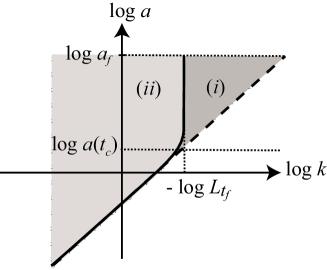
Figure 4: The dark grey region represents the region (i). The light grey region represents the region (ii). These two regions are divided by the solid curve which shows the scale of the causally connected region, i.e., $k=L_{t}^{-1}$. The dashed line is the horizon scale, i.e., $k=a(t)H(t)$, which corresponds to the effective UV cutoff scale.

We discriminate the region (ii) in which the operation of $\hat{\bar{W}}_{t}$ results in an additional suppression of amplitude from the region (i) in which it does not.

Let us consider first the region (i). In this case, as is obvious from Fig. 4, the time integration is restricted to $t^{\prime}\gtrsim t_{c}$. Hence, we have $L_{t^{\prime}}\approx L_{t}\approx L_{t_{f}}$. Furthermore, since $t_{c}$ is not so far from $t_{f}$, we can approximate $H(t^{\prime})$ by $H(t)$. Hence, for $n<n_{c}$ we obtain

$$\left|C[\hat{G}_{R}(W_{t^{\prime}}\Gamma_{n})]_{\hbox{\boldmath{\scriptsize$k$}}}\right| \!\!\lesssim \!\!\int^{a(t)}_{a(t_{k})}\!{da(t^{\prime})\over a(t^{\prime})}L_{t^{\prime}}^{3}\Bigl{(}\frac{H(t^{\prime})}{M_{\rm pl}}\Bigr{)}^{n}$$

$$\simeq L_{t}^{3}\left({H(t)\over M_{\rm pl}}\right)^{n}\log(a(t)/a(t_{c}))~{}.$$

Since $\log(a(t)/a(t_{c}))$ cannot be a large number, this inequality means that $C[\hat{G}_{R}(W_{t^{\prime}}\Gamma_{n})]=O([H(t)/M_{\rm pl}]^{n})$. A parallel argument holds for $n>n_{c}$, too.

Next, we consider the region (ii). To consider this region, it is essential to take into account the operation of $\hat{\bar{W}}_{t}$. Using the relation (95), we have

$$C[\hat{\bar{W}}_{t}\!\!\! \hat{G}_{R}\!\!\! (W_{t^{\prime}}\Gamma_{n})]$$ (96)

$$\!\!\lesssim \!\!\int\!{da(t^{\prime})\over a(t^{\prime})}\int_{k<L_{t^{\prime}}^{-1}}{d^{3}\!k\over(2\pi)^{3}}$$ (98)

$$\times\left(e^{i{\hbox{\boldmath{\scriptsize$k$}}}\cdot{\hbox{\boldmath{\scriptsize$x$}}}}-{W_{t,-{\hbox{\boldmath{\scriptsize$k$}}}}\over W_{t,{\hbox{\boldmath{\scriptsize$0$}}}}}\right)L_{t^{\prime}}^{3}\left[{H(t^{\prime})\over M_{\rm pl}}\right]^{n}~{}.$$

Here we have changed the order of integrations.

As we consider the region $k\lesssim L_{t}^{-1}$, $W_{t,-{\hbox{\boldmath{\scriptsize$k$}}}}/W_{t,{\hbox{\boldmath{\scriptsize$0$}}}}$ will be expanded as $W_{t,-{\hbox{\boldmath{\scriptsize$k$}}}}/W_{t,{\hbox{\boldmath{\scriptsize$0$}}}}=1+O((L_{t}k)^{2})$. Therefore the factor $\hat{\bar{W}}_{t}e^{i{\hbox{\boldmath{\scriptsize$k$}}}\cdot{\hbox{\boldmath{\scriptsize$x$}}}}=e^{i{\hbox{\boldmath{\scriptsize$k$}}}\cdot{\hbox{\boldmath{\scriptsize$x$}}}}-{W_{t,-{\hbox{\boldmath{\scriptsize$k$}}}}/W_{t,{\hbox{\boldmath{\scriptsize$0$}}}}}$ is approximated by $i{\bm{k}}\cdot{\bm{x}}$. Then, performing the momentum integration, we obtain

$$\left|C[\hat{\bar{W}}_{t}\hat{G}_{R}(W_{t^{\prime}}\Gamma_{n})]\right|\lesssim L_{t}\int\!{da(t^{\prime})\over a(t^{\prime})}L_{t^{\prime}}^{-1}\left[{H(t^{\prime})\over M_{\rm pl}}\right]^{n}\!\!,$$ (100)

where we have used $|{\bm{x}}|\lesssim L_{t}$. For small $a(t^{\prime})$, $L_{t^{\prime}}^{-1}\approx a(t^{\prime})H(t^{\prime})$. Thus we find that the integrand $L^{-1}_{t^{\prime}}(H/M_{\rm pl})^{n}$ is proportional to $(aH)H^{n}\propto a^{1-(n+1)\epsilon}$. For $n<n_{c}=\epsilon^{-1}-1$, the integration is dominated by the later epoch. Hence, we have an estimate $C[\hat{\bar{W}}_{t}\hat{G}_{R}(W_{t^{\prime}}\Gamma_{n})]=O\left(\left[{H(t)/M_{\rm pl}}\right]^{n}\right)$. For $n>n_{c}=\epsilon^{-1}-1$, there are terms whose order of magnitude is bounded by

$$(a_{i}H_{i}L_{t})\left[{H_{i}\over M_{\rm pl}}\right]^{n-1}\!\int\!{da(t^{\prime})\over a(t^{\prime})}{H(t^{\prime})\over M_{\rm pl}},$$

or

$$(a_{i}H_{i}L_{t})\left[{H_{i}\over M_{\rm pl}}\right]^{n}\!\int\!{da(t^{\prime})\over a(t^{\prime})}(a_{i}H_{i}L_{t^{\prime}}),$$

besides the terms that are estimated as in Eq. (100). In all cases the time integration is dominated by the earlier epoch. Thus, we have an estimate $C[\hat{\bar{W}}_{t}\hat{G}_{R}(W_{t^{\prime}}\Gamma_{n})]=O\left((a_{i}H_{i}L_{t})\left[{H_{i}/M_{\rm pl}}\right]^{n}\right)~{}.$ We find that the initial time dependence remains in $C[\tilde{\varphi}_{n}]$ for $n>n_{c}$, but it has at least one suppression factor $(a_{i}H_{i}L_{t})$ associated. To conclude, we have shown that the condition (83) is satisfied in all cases.

Before closing this section, we would like to stress the importance of the factor $\hat{\bar{W}}_{t}e^{i{\hbox{\boldmath{\scriptsize$k$}}}\cdot{\hbox{\boldmath{\scriptsize$x$}}}}$ in Eq.( LABEL:important1), which is absent in the standard treatment. This factor is the origin of the factor $L_{t}/L_{t^{\prime}}$ in Eq. (100). If it were not for this factor, this integral would be dominated by the earlier epoch for any $n$. (In the slow-roll limit $\epsilon\to 0$, the integral would be proportional to the $e$-holding number $N=\log a(t)/a(t_{i})$.) Hence, the initial time dependence appears in the $n$-point functions even for small $n$ at the lowest tree-level order.

Even if we follow our improved prescription, the contribution from $\tilde{\varphi}_{n}$ with $n>n_{c}$ carries the dependence on the artificial choice of the initial time $t_{i}$. Physical origin of this dependence on $t_{i}$ is clear. This dominance of the contribution from the earlier epoch originates simply from larger amplitude of fluctuation due to larger $H$. Even if the propagation of fluctuation from far past is suppressed, the source $\Gamma_{n}$ rapidly increases toward the past for large $n$. Therefore we suspect that this initial time dependence might be really physical, although it appears only when we consider sufficiently higher order perturbations. However, as we have not used all the residual gauge degrees of freedom, there might be a better prescription for the gauge fixing in which the critical order $n_{c}$ is larger.

IV Conclusion

As the possibility of detecting nonlinearities in the primordial perturbations of the universe is increasing, it becomes more important to understand the issue of IR divergences in the computation of primordial perturbations and to predict their finite amplitude that we actually observe Komatsu:2008hk . In this paper, we pointed out that the standard prescription of the cosmological perturbation theory contains residual gauge degrees of freedom if the gauge conditions are imposed only locally within our observable universe, and that it is important to fix these gauge degrees of freedom to remove IR divergences. In order to fix the residual gauge degrees of freedom, taking the boundary conditions which shut off the influence from the unobservable region, we proposed the use of local gauge fixing conditions.

When we have an equation of elliptic type, the boundary conditions are not arbitrary in general. If we change the boundary conditions for an elliptic type equation, we obtain a different solution. However, here the elliptic type equations appear only for determining the lapse function and the shift vector. The boundary conditions in solving the elliptic type equations are not specified from the flat gauge condition alone. A different choice of the boundary conditions corresponds to a different way of fixing the residual gauge degrees of freedom. Our choice of local gauge conditions is not unique, but it completely fixes the gauge in ${\cal O}$ without using any information outside ${\cal O}^{\prime}$.

It is true that the $n$-point functions calculated in the present manner depend on the choice of fixing the residual gauge. Making use of the transfer functions, any real observables like the angular power spectrum of the CMB sky map can be described in terms of these $n$-point functions for the primordial perturbations observables . For the single field inflation model, we have shown that the amplitude of our primordial perturbations is free from IR divergences (unless the Hubble parameter at the initial time is well below the Planck scale). Then, the real observables should be also IR regular. We also pointed out the possibility that the terms which depend on the initial time may dominate in higher order perturbations above a critical order.

At the end of this paper, let us comment on the case in which more than one fields participate in IR divergences. In our proof of the absence of IR divergences we used the gauge in which the local average of the inflaton field does not fluctuate using one of the residual gauge degrees of freedom mentioned above. This adjustment of the average value is possible only for one field. When plural fields have scale invariant or even redder spectra, therefore our prescription presented here is not enough to regularize IR divergences. This claim is on the same line with the argument given by G. Geshnizjani and R. Brandenberger in Geshnizjani:2002wp ; Geshnizjani:2003cn . Discussing the backreaction on the background expansion rate due to classical fluctuations, they showed that the observable expansion rate does not suffer from cumulative backreaction in single-component models, while it does in multi-component models.

Thus, when plural fields are concerned with IR divergences, we need more careful discussion about what we actually observe. When we consider the eternal inflation scenario, the wave function of the universe is infinitely spread in the field space, and the expectation values of field fluctuations will diverge. We think that these divergences due to the fields other than inflaton are physical. However, in the actual observation of the universe we will not see any divergences. The key idea will be that what we compute as the correlation functions in field theory are different from what we really observe. We think that in this case it is essential to take into account the decoherence effects in order to remove these IR divergences. Deferring the detailed explanation to the succeeding paper IRmulti , we describe here our basic idea how to handle the divergences in the multi-field case briefly. We focus on the field whose IR corrections still diverge even after the local gauge fixing. We denote it by $\varphi_{IR}$. The adiabatic vacuum state can be decomposed into a superposition of wave packets which have a peak at a certain value of the local average $\hat{W}_{t}\varphi_{IR}(\tau_{f})$. As the universe evolves, the wave packets lose correlation to each other. Through this so-called decoherence process, the coherent superposition of the wave packets starts to behave as a statistical ensemble of many different worlds, where each world means the universe described by a decohered wave packet Polarski:1995jg ; Kiefer:2006je ; Starobinsky:1986fx . Our observed world is just a representative one expressed by a wave packet randomly chosen from various possibilities. Once one wave packet is selected after the decoherence process, the evolution of our world will not be affected by the other parallel worlds. However, the initial vacuum state does include the contributions from all the wave packets. This implies that a naive computation of $n$-point functions is contaminated by the contribution from the other worlds uncorrelated to ours, which is the origin of the divergences.

Recently the stochastic approach Starobinsky:1986fx ; Starobinsky:1994bd ; Nakao:1988yi ; Nambu:1988je ; Morikawa:1989xz ; Morikawa:1987ci ; Tanaka:1997iy has been employed in order to solve the IR divergence problem Bartolo:2007ti ; Riotto:2008mv ; Enqvist:2008kt . This is in harmony with our claim. However, it is hard to deny the spiteful suspicion that the reason why the problem of IR divergence does not appear in the stochastic approach might be simply because quantum fluctuations in the IR limit are neglected by hand. Therefore, in our succeeding paper, we describe the decoherence effect without relying on the stochastic approach, and discuss the regularity of the IR corrections.

In contrast, when we consider the case in which only a single field is responsible for IR divergences, using the residual gauge degrees of freedom, we can adjust the local average value of the field not to fluctuate. Then, as we have shown in this paper, we need not to pick-up one decohered wave packet from the superposition of infinitely many wave packets.

- (1) J. E. Lidsey, A. R. Liddle, E. W. Kolb, E. J. Copeland, T. Barreiro and M. Abney, Rev. Mod. Phys. 69, 373 (1997) [arXiv:astro-ph/9508078].
- (2) B. A. Bassett, S. Tsujikawa and D. Wands, Rev. Mod. Phys. 78, 537 (2006) [arXiv:astro-ph/0507632].
- (3) D. H. Lyth, Lect. Notes Phys. 738, 81 (2008) [arXiv:hep-th/0702128].
- (4) A. Linde, Lect. Notes Phys. 738, 1 (2008) [arXiv:0705.0164 [hep-th]].
- (5) N. Bartolo, S. Matarrese and A. Riotto, Phys. Rev. D 65, 103505 (2002) [arXiv:hep-ph/0112261].
- (6) N. Bartolo, E. Komatsu, S. Matarrese and A. Riotto, Phys. Rept. 402, 103 (2004) [arXiv:astro-ph/0406398].
- (7) J. M. Maldacena, JHEP 0305, 013 (2003) [arXiv:astro-ph/0210603].
- (8) S. A. Kim and A. R. Liddle, Phys. Rev. D 74, 063522 (2006) [arXiv:astro-ph/0608186].
- (9) D. Babich, P. Creminelli and M. Zaldarriaga, JCAP 0408, 009 (2004) [arXiv:astro-ph/0405356].
- (10) D. Seery and J. E. Lidsey, JCAP 0506, 003 (2005) [arXiv:astro-ph/0503692].
- (11) D. Seery and J. E. Lidsey, JCAP 0509, 011 (2005) [arXiv:astro-ph/0506056].
- (12) S. Weinberg, Phys. Rev. D 72, 043514 (2005) [arXiv:hep-th/0506236].
- (13) S. Weinberg, Phys. Rev. D 74, 023508 (2006) [arXiv:hep-th/0605244].
- (14) G. I. Rigopoulos, E. P. S. Shellard and B. J. W. van Tent, Phys. Rev. D 73, 083521 (2006) [arXiv:astro-ph/0504508].
- (15) G. I. Rigopoulos, E. P. S. Shellard and B. J. W. van Tent, Phys. Rev. D 73, 083522 (2006) [arXiv:astro-ph/0506704].
- (16) G. I. Rigopoulos, E. P. S. Shellard and B. J. W. van Tent, Phys. Rev. D 76, 083512 (2007) [arXiv:astro-ph/0511041].
- (17) F. Vernizzi and D. Wands, JCAP 0605, 019 (2006) [arXiv:astro-ph/0603799].
- (18) X. Chen, M. x. Huang, S. Kachru and G. Shiu, JCAP 0701, 002 (2007) [arXiv:hep-th/0605045].
- (19) T. Battefeld and R. Easther, JCAP 0703, 020 (2007) [arXiv:astro-ph/0610296].
- (20) S. Yokoyama, T. Suyama and T. Tanaka, Phys. Rev. D 77, 083511 (2008) [arXiv:0711.2920 [astro-ph]].
- (21) S. Yokoyama, T. Suyama and T. Tanaka, JCAP 0902, 012 (2009) [arXiv:0810.3053 [astro-ph]].
- (22) D. Seery, M. S. Sloth and F. Vernizzi, arXiv:0811.3934 [astro-ph].
- (23) A. Naruko and M. Sasaki, Prog. Theor. Phys. 121, 193 (2009) [arXiv:0807.0180 [astro-ph]].
- (24) S. Weinberg, arXiv:0805.3781 [hep-th].
- (25) S. Weinberg, Phys. Rev. D 78, 123521 (2008) [arXiv:0808.2909 [hep-th]].
- (26) S. Weinberg, arXiv:0810.2831 [hep-ph].
- (27) H. R. S. Cogollo, Y. Rodriguez and C. A. Valenzuela-Toledo, JCAP 0808, 029 (2008) [arXiv:0806.1546 [astro-ph]].
- (28) Y. Rodriguez and C. A. Valenzuela-Toledo, arXiv:0811.4092 [astro-ph].
- (29) D. Boyanovsky and H. J. de Vega, Phys. Rev. D 70, 063508 (2004) [arXiv:astro-ph/0406287].
- (30) D. Boyanovsky, H. J. de Vega and N. G. Sanchez, Phys. Rev. D 71, 023509 (2005) [arXiv:astro-ph/0409406].
- (31) D. Boyanovsky, H. J. de Vega and N. G. Sanchez, Nucl. Phys. B 747, 25 (2006) [arXiv:astro-ph/0503669].
- (32) D. Boyanovsky, H. J. de Vega and N. G. Sanchez, Phys. Rev. D 72, 103006 (2005) [arXiv:astro-ph/0507596].
- (33) V. K. Onemli and R. P. Woodard, Class. Quant. Grav. 19, 4607 (2002) [arXiv:gr-qc/0204065].
- (34) T. Brunier, V. K. Onemli and R. P. Woodard, Class. Quant. Grav. 22, 59 (2005) [arXiv:gr-qc/0408080].
- (35) T. Prokopec, N. C. Tsamis and R. P. Woodard, arXiv:0707.0847 [gr-qc].
- (36) M. S. Sloth, Nucl. Phys. B 748, 149 (2006) [arXiv:astro-ph/0604488].
- (37) M. S. Sloth, Nucl. Phys. B 775, 78 (2007) [arXiv:hep-th/0612138].
- (38) D. Seery, JCAP 0711, 025 (2007) [arXiv:0707.3377 [astro-ph]].
- (39) D. Seery, JCAP 0802, 006 (2008) [arXiv:0707.3378 [astro-ph]].
- (40) Y. Urakawa and K. i. Maeda, Phys. Rev. D 78, 064004 (2008) [arXiv:0801.0126 [hep-th]].
- (41) N. Afshordi and R. H. Brandenberger, Phys. Rev. D 63, 123505 (2001) [arXiv:gr-qc/0011075].
- (42) K. c. Chou, Z. b. Su, B. l. Hao and L. Yu, Phys. Rept. 118, 1 (1985).
- (43) R. D. Jordan, Phys. Rev. D 33, 444 (1986).
- (44) E. Calzetta and B. L. Hu, Phys. Rev. D 35, 495 (1987).
- (45) E. Komatsu et al. [WMAP Collaboration], arXiv:0803.0547 [astro-ph].
- (46) In this paper, we refered to the primordial fluctuation in the local flat gauge as the observable fluctuation. However, strictly speaking, this fluctuation cannot be directly observed. To obtain the expression for what we actually observe through some measurement, such as the CMB angular power spectrum, we need further computations. However, if the correlation functions of the primordial fluctuation that we discussed here are free from IR divergences, the true observables are also guaranteed to be so.
- (47) G. Geshnizjani and R. Brandenberger, Phys. Rev. D 66, 123507 (2002) [arXiv:gr-qc/0204074].
- (48) G. Geshnizjani and R. Brandenberger, JCAP 0504, 006 (2005) [arXiv:hep-th/0310265].
- (49) Y. Urakawa and T. Tanaka, arXiv:0904.4415 [hep-th].
- (50) D. Polarski and A. A. Starobinsky, Class. Quant. Grav. 13, 377 (1996) [arXiv:gr-qc/9504030].
- (51) C. Kiefer, I. Lohmar, D. Polarski and A. A. Starobinsky, Class. Quant. Grav. 24, 1699 (2007) [arXiv:astro-ph/0610700].
- (52) A. A. Starobinsky, Lect. Notes Phys. 246, 107 (1986).
- (53) A. A. Starobinsky and J. Yokoyama, Phys. Rev. D 50, 6357 (1994) [arXiv:astro-ph/9407016].
- (54) K. i. Nakao, Y. Nambu and M. Sasaki, Prog. Theor. Phys. 80, 1041 (1988).
- (55) Y. Nambu and M. Sasaki, Phys. Lett. B 219, 240 (1989).
- (56) M. Morikawa, Phys. Rev. D 42, 1027 (1990).
- (57) M. Morikawa, Prog. Theor. Phys. 77, 1163 (1987).
- (58) T. Tanaka and M. a. Sakagami, Prog. Theor. Phys. 100, 547 (1998) [arXiv:gr-qc/9705054].
- (59) D. H. Lyth, JCAP 0712, 016 (2007) [arXiv:0707.0361 [astro-ph]].
- (60) N. Bartolo, S. Matarrese, M. Pietroni, A. Riotto and D. Seery, JCAP 0801, 015 (2008) [arXiv:0711.4263 [astro-ph]].
- (61) A. Riotto and M. S. Sloth, JCAP 0804, 030 (2008) [arXiv:0801.1845 [hep-ph]].
- (62) K. Enqvist, S. Nurmi, D. Podolsky and G. I. Rigopoulos, JCAP 0804, 025 (2008) [arXiv:0802.0395 [astro-ph]].