Coverage in Multi-Antenna Two-Tier Networks

Abstract

In two-tier networks – comprising a conventional cellular network overlaid with shorter range hotspots (e.g. femtocells, distributed antennas, or wired relays) – with universal frequency reuse, the near-far effect from cross-tier interference creates dead spots where reliable coverage cannot be guaranteed to users in either tier. Equipping the macrocell and femtocells with multiple antennas enhances robustness against the near-far problem. This work derives the maximum number of simultaneously transmitting multiple antenna femtocells meeting a per-tier outage probability constraint. Coverage dead zones are presented wherein cross-tier interference bottlenecks cellular and femtocell coverage. Two operating regimes are shown namely 1) a cellular-limited regime in which femtocell users experience unacceptable cross-tier interference and 2) a hotspot-limited regime wherein both femtocell users and cellular users are limited by hotspot interference. Our analysis accounts for the per-tier transmit powers, the number of transmit antennas (single antenna transmission being a special case) and terrestrial propagation such as the Rayleigh fading and the path loss exponents. Single-user (SU) multiple antenna transmission at each tier is shown to provide significantly superior coverage and spatial reuse relative to multiuser (MU) transmission. We propose a decentralized carrier-sensing approach to regulate femtocell transmission powers based on their location. Considering a worst-case cell-edge location, simulations using typical path loss scenarios show that our interference management strategy provides reliable cellular coverage with about $60$ femtocells per cellsite.

I Introduction

Wireless operators are in the process of augmenting the macrocell network with supplemental infrastructure such as microcells, distributed antennas and relays. An alternative with lower upfront costs is to improve indoor coverage and capacity using the concept of end-consumer installed femtocells or home base stations[1]. A femtocell is a low power, short range ($10-50$ meters) wireless data access point (AP), functioning in service provider owned licensed spectrum, which provides in-building coverage to home users and transports the user traffic over internet based backhaul such as cable modem. Because of the proximity of users to their APs, femtocells provide higher spatial reuse of spectrum and cause less interference to other users. The spatial reuse (in $\mathrm{b/s/Hz/m^{2}}$) is readily expressible by the area spectral efficiency (ASE) [2] which is a measure of the total obtainable network throughput per unit Hz per unit area. Previous studies[1] have shown a nearly $25$x improvement in overall spatial reuse when moving from a macrocell-only network to a two-tier underlay with $50$ femtocells per cellsite.

In addition to improved spatial reuse, cellular operators desire to operate both cellular and indoor femtocell users in the same bandwidth (termed universal frequency reuse), as is assumed in this paper, for cost effectiveness and flexible deployment [3]. With shared spectrum, practical challenges stem from the absence of coordination across tiers [1, 4] due to scalability issues. Because femtocells are consumer deployed in their self-interest and because of reasons of security and limited backhaul capacity, these femtocells will potentially offer privileged coverage only to licensed, subscribed indoor users. This paper assumes Closed Access (CA), which means only licensed home users within radio range can communicate with their own femtocell. The drawback of such a co-channel closed access deployment of femtocells is that cross-tier interference becomes the capacity-limiting factor. For example, a cellular user located at the edge of their macrocell may experience unacceptable interference from an actively transmitting femtocell in vicinity. Commercial femtocell offerings (such as Verizon’s “home network expander”) provide both public access and closed access operation which are user configurable. Our results provide a networkwide performance benchmark in a closed access setting.

I-A Problem Definition

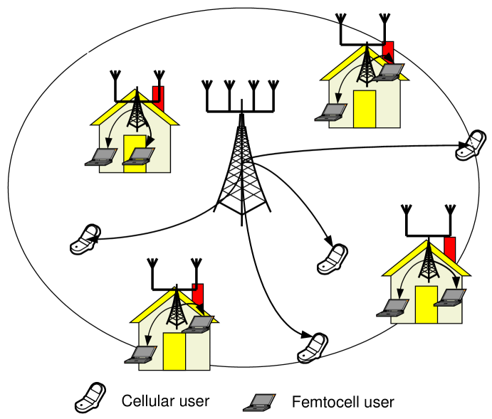
Figure 1: Multiuser multiple antenna transmission in a two-tier network.

The motivation behind this paper is to understand how exploiting the available degrees of freedom through multiple antenna transmission influences coverage and spatial reuse in a two-tier network with universal frequency reuse. We consider both single-user (SU) multiple antenna transmission and multiuser (MU) multiple antenna transmission (Fig. 1) employed by the macrocell basestation (BS) and femtocell APs. Array gain resulting from SU transmission provides robustness against cross-tier interference. Multiuser transmission, on the other hand, increases the number of simultaneous transmissions at the expense of reduced signal strength per user terminal and potential inter-user interference.

Given a multiple antenna transmission strategy (SU or MU), let $\lambda_{f}$ denote the maximum density (in femtocells per square meter) of simultaneously transmitting femtocells – denoted as the maximum femtocell contention density – that guarantees a certain minimum per-tier Quality of Service (QoS) requirement. Given a certain minimum per-tier target Signal-to-Interference Ratio (SIR) equaling $\Gamma$, the QoS requirement stipulates that the instantaneous SIR at each user should exceed $\Gamma$ with a probability of at least $1-\epsilon$, where $\epsilon$ is a design parameter. Since the signal power for a cellular user decays as $D^{-\alpha_{c}}$ ($D$ being the distance from the macrocell BS and $\alpha_{c}$ is the outdoor path loss exponent), satisfying its QoS requirement requires $\lambda_{f}$ to be a monotonically decreasing function of $D$. Conversely, satisfying the QoS requirement for a femtocell user at $D$ necessitates $\lambda_{f}$ to be monotonically decreasing as $D\rightarrow 0$.

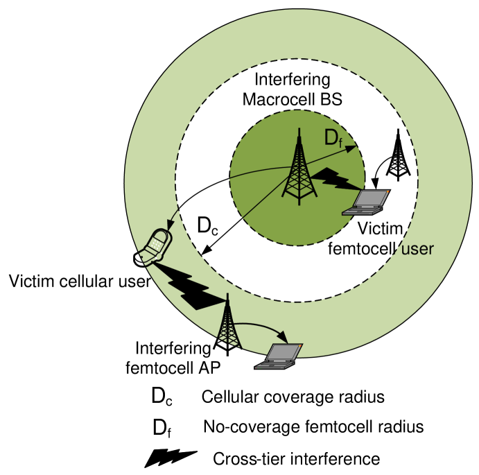
Figure 2: No-coverage femtocell radius and cellular coverage radius in a two-tier network with cochannel deployment.

This paper characterizes near-far effects and the resulting per-tier coverage by defining two quantities of interest namely the No-Coverage Femtocell Radius and the Cellular Coverage Radius. The no-coverage femtocell radius $D_{f}$ determines the minimum SIR feasible femtocell distance from the macrocell (see Fig. 2). Any femtocell user within $D<D_{f}$ meters from the macrocell experiences an outage probability greater than $\epsilon$ due to excessive cellular interference. This suggests that any user at $D<D_{f}$ should communicate with the macrocell because of its potentially higher cellular SIR. The cellular coverage radius $D_{c}$ denotes the maximum SIR feasible distance from the macrocell up to which a cellular user can satisfy its outage probability constraint in the presence of hotspot interference. Since there is no coordination between tiers for managing interference, providing greater spatial reuse using femtocells trades off the coverage radii and vice-versa. Because the cellular network serves as the primary network to mobile outdoor users, it is desirable to maximize $D_{c}$ in the presence of hotspot interference.

Assuming that each tier employs either transmit beamforming (BF) [for SU transmission] or linear zero-forcing precoding [for MU transmission] with transmission powers $P_{c}$ and $P_{f}$ in each resource (eg. frequency sub-band), this work poses the following questions:

• What is the maximum femtocell contention density $\lambda_{f}$ as a function of the location $D$ with respect to (w.r.t) the macrocell BS, the ratio $P_{c}/P_{f}$, the transmission strategy (SU vs. MU transmission), the number of transmit antennas per macrocell BS and femtocell AP, the target per-tier SIR $\Gamma$, the maximum outage probability $\epsilon$ and the path loss exponents?

• Given an average of $N_{f}$ transmitting femtocells per cell-site, how much cellular coverage can the macrocell BS provide to its users?

• How does the no-coverage femtocell radius vary with SU and MU transmission strategies?

• How should femtocells adapt their transmission power for ensuring reliable cellular coverage?

I-B Related Work

Prior research in tiered networks have mainly considered an operator planned underlay of a macrocell with single/multiple microcells[5, 6]. A microcell has a much larger radio range (100-500 m) than a femtocell, and generally implies centralized deployment, i.e. by the service-provider. This allows the operator to either load balance users or preferentially assign high data rate cellular users to the microcell [7, 8] because of its inherently larger capacity. In contrast, femtocells are consumer installed and the traffic requirements at femtocells are user determined without any operator influence. Consequently, decentralized strategies for interference management may be preferred[9, 1, 10, 11].

The subject of this work is related to Huang et al.[12] which derives per-tier transmission capacities with spectrum underlay and spectrum overlay. In contrast to their work which assumes relay-assisted cell-edge users, our work proposes to improve coverage by regulating femtocell transmit powers. Hunter et al.[13] have derived transmission capacities in an ad hoc network with spatial diversity. Our work has extended this analysis to a cellular-underlaid ad hoc network.

Finally, related works on cognitive radios (CR) include (but not restricted to) 1. analyzing sensing-throughput tradeoffs[14] for computing optimal sensing time by CR users and 2. limit transmit powers of CR users[15, 16, 17, 18] . The differentiating aspect of our work is a decentralized femtocell transmit power selection scheme which ensures a per-tier outage probability below a desired threshold.

I-C Contributions

Given $T_{c}$ antennas at the macrocell BS and $T_{f}$ antennas per femtocell AP, a maximum tolerable per-tier outage probability $\epsilon$ and path loss exponents $\alpha_{c}$ (outdoor cellular transmission) and $\alpha_{fo}$ (during indoor-to-outdoor femtocell transmission) respectively, this work provides the following contributions.

Coverage.

We derive coverage zones wherein cross-tier interference prevents users in each tier from satisfying their QoS requirements. Single-user macrocell transmission is shown to increase the cellular coverage radius by a factor $T_{c}^{2/\alpha_{c}}$ relative to MU transmission. Single-user femtocell transmission is shown to decrease the no-coverage femtocell radius $D_{f}$ by a factor of $(T_{f}/\epsilon^{1-1/T_{f}})^{1/\alpha_{c}}$ relative to MU femtocell transmission. This suggests that SU transmission results in superior coverage in either tier. We also show that femtocell performance is regulated by cellular interference and hotspot interference is negligible in comparison.

Hotspot Contention Density.

We derive the maximum femtocell contention density $\lambda_{f}^{\ast}(D)$ at distance $D$ from the macrocell BS. Two distinct operating regimes are shown namely a 1. Cellular-limited regime, wherein femtocell users are primarily affected by cellular interference and 2. Hotspot-limited regime wherein both cellular and hotspot users are affected by hotspot interference . Regime 1 determines the coverage provided to femtocell users, while Regime 2 determines $\lambda_{f}^{\ast}(D)$ and the cellular coverage radius. In Regime 2, SU macrocell transmission is shown to increase $\lambda_{f}^{\ast}(D)$ by a factor of $\mathbf{\Gamma}(1-2/\alpha_{fo})T_{c}^{4/\alpha_{fo}}$ (where $\mathbf{\Gamma}(z)\triangleq\int_{0}^{\infty}t^{z-1}e^{-t}\textrm{ d}t\ \forall\textrm{Re}(t)>0$ is the Gamma function) relative to MU transmission. Femtocells maximize their area spectral efficiency by choosing their transmission strategy depending on $\alpha_{fo}$, with SU transmission being desirable with considerable hotspot interference ($\alpha_{fo}<4$). This suggests that per-tier SU transmission is preferable from a spatial reuse perspective.

Power control.

We propose a carrier-sensing approach in which a femtocell chooses its transmit power depending on its distance from the macrocell BS for minimizing cross-tier interference. This strategy provides reliable cellular coverage with up to 60 femtocells per cell site (with typical cellular parameters).

II System Model

Assume a central macrocell $B_{0}$ using $T_{c}$ antennas to service a geographical region $\mathcal{C}$, assumed as a circular disc with radius $R_{c}$ and area $|\mathcal{C}|=\pi R_{c}^{2}$. Each femtocell is equipped with $T_{f}$ antennas. Femtocell users are located on the circumference of a disc of radius $R_{f}$ centered at their femtocell AP. Both cellular users and femtocell users are assumed to be equipped with single-antenna receivers. In a given time/frequency slot, each macrocell [resp. femtocell] employs its $T_{c}$ [resp. $T_{f}$] antennas for serving $1\leq U_{c}\leq T_{c}$ cellular [resp. $1\leq U_{f}\leq T_{f}$ indoor] users. Although user selection has a potentially beneficial impact, it is not considered in this work for analytical tractability.

This paper employs a stochastic geometry framework for modeling the random spatial distribution of the underlying femtocells. Hotspot locations are likely to vary from one cell site to another, and be opportunistic rather than planned, so an analysis that embraces instead of neglecting randomness should provide more accurate results and more plausible insights. The randomly located femtocells are assumed to be distributed according to a Spatial Poisson Point Process (SPPP) $\Pi_{f}$ (see [19, 20] for background, prior works include [21, 22, 23]). Provided $\Pi_{f}$ is a homogeneous SPPP (or the intensity $\lambda_{f}$ in femtocells per square meter stays constant over $\mathcal{C}$), the average number of actively transmitting femtocells is readily obtained as $N_{f}=\lambda_{f}|\mathcal{C}|$ femtocells per cellsite. Because of near-far effects inherent to a two-tier network, the maximum hotspot intensity varies with the location $D$ in the cell-site.

II-A Terrestrial Path Loss Model

The signal decay encountered using terrestrial propagation to users in either tier is represented using a distance based path loss model. Temporal amplitude variations of the complex vector downlink channel are modeled as frequency-flat Rayleigh fading – e.g. each frequency sub-band in frequency division multiple access (FDMA) transmission – with individual complex entries distributed as $\mathcal{CN}(0,1)$. For analytical simplicity, this work does not consider random lognormal shadow fading. Instead, we shall assume a fixed partition loss encountered during outdoor-to-indoor and indoor-to-indoor wireless propagation. Shown below, we use the IMT-2000 channel model[24, Page 26] for modeling indoor losses (based on the COST231 indoor model[24, Page 44]) and outdoor path losses.

Macrocell to Cellular Users.

The decibel path loss between $B_{0}$ and cellular user $0$ is modeled as $\mathrm{PL}_{c,\textrm{dB}}=A_{c,\textrm{dB}}+10\alpha_{c}\log_{10}D$ where $\alpha_{c}$ is the outdoor path loss exponent, $A_{c,\textrm{dB}}=30\log_{10}f_{c}-71$ represents the fixed decibel loss during outdoor propagation, $f_{c}$ is the carrier frequency in MHz and $D$ is the distance between $B_{0}$ and its user.

Macrocell to Femtocell Users.

We model each femtocell as a point object, hence all indoor users served by a given femtocell experience identical path loss from cellular interference. This decibel path loss is given as $\mathrm{PL}_{f,c,\textrm{dB}}=A_{f,c,\textrm{dB}}+10\alpha_{c}\log_{10}(D)$ where $A_{f,c,\textrm{dB}}=30\log_{10}f_{c}-71+W_{\textrm{dB}}$ designates the fixed decibel path loss, $D$ is the distance between $B_{0}$ and the femtocell and $W_{\textrm{dB}}$ equals the decibel wall partition loss during outdoor-to-indoor wireless propagation.

Femtocell to Subscribed Home Users.

The decibel path loss between a femtocell to its licensed, subscribed indoor users is modeled as $\mathrm{PL}_{fi,\textrm{dB}}=A_{fi,\textrm{dB}}+10\alpha_{fi}\log_{10}(R_{f})$ where $A_{fi,\textrm{dB}}=37$ dB models the fixed propagation loss in decibels between the femtocell to its desired user, $\alpha_{fi}$ represents the indoor path loss exponent.

Femtocell to Outdoor Cellular Users.

Given a transmitting femtocell, any cellular user located at distance $D$ will experience cross-tier interference with decibel path loss modeled as $\mathrm{PL}_{c,f\textrm{dB}}=A_{c,f,\textrm{dB}}+10\alpha_{fo}\log_{10}(D)$. Here, the fixed decibel path loss is designated by $A_{c,f,\textrm{dB}}=P_{\textrm{dB}}+37$, while $\alpha_{fo}$ denotes the path loss exponent during indoor-to-outdoor wireless propagation.

Femtocell to Neighboring Femtocells.

The decibel path loss of the hotspot interference caused by a transmitting femtocell at another femtocell is given as $\mathrm{PL}_{f,f\textrm{dB}}=A_{f,f,\textrm{dB}}+10\alpha_{fo}\log_{10}(D)$ where $A_{f,f,\textrm{dB}}=2W_{\textrm{dB}}+37$ denotes the fixed decibel path loss (the factor of $2$ models the double wall partition loss during indoor to indoor propagation) and $D$ is the distance between the two femtocells.

III Per-Tier Signal-to-Interference Ratios

Assume that the macrocell $B_{0}$ serves $1\leq U_{c}\leq T_{c}$ users. Define $\mathbf{h}_{j}\in\mathbb{C}^{T_{c}\times 1}$ as the channel from $B_{0}$ to cellular user $j\in\{0,1,\dots,U_{c}-1\}$ with its entries distributed as $h_{k,j}\sim\mathcal{CN}(0,1)$. The direction of each vector channel is represented as $\tilde{\mathbf{h}}_{j}\triangleq\frac{\mathbf{h}_{j}}{||\mathbf{h}_{j}||}$. Designate $\tilde{\mathbf{H}}=[\tilde{\mathbf{h}}_{0},\ \tilde{\mathbf{h}}_{1},\ \dots,\ \tilde{\mathbf{h}}_{U_{c}-1}]^{\dagger}\in\mathbb{C}^{U_{c}\times T_{c}}$ as the concatenated matrix of channel directions, where the symbol $\dagger$ denotes conjugate transpose.

AS 1

Perfect channel state information (CSI) is assumed at the central macrocell [resp. femtocells] regarding the channels to their own users.

Although we acknowledge that imperfect channel estimation plays a potentially significant role, we defer its analysis for subsequent research and instead employ AS1 for analytical tractability.

AS 2

For analytical tractability, interference from neighboring macrocell BSs is ignored.

This work assumes linear zero-forcing (ZF) precoding transmission because it has low complexity, yet achieves the same multiplexing gain as higher complexity schemes such as dirty-paper coding. With ZF precoding transmission, macrocell BS $B_{0}$ chooses its precoding matrix $\mathbf{V}\in\mathbb{C}^{T_{c}\times U_{c}}=[\mathbf{v}_{i}]_{1\leq i\leq U_{c}}$ as the normalized columns of the pseudoinverse $\tilde{\mathbf{H}}^{\dagger}(\tilde{\mathbf{H}}\tilde{\mathbf{H}}^{\dagger})^{-1}\in\mathbb{C}^{T_{c}\times U_{c}}$. Similarly, each femtocell $F_{j}\in\Pi_{F}$ serves $1\leq U_{f}\leq T_{f}$ users with the channel directions between $F_{j}$ to its individual users represented as $\tilde{\mathbf{G}}_{j}=[\tilde{\mathbf{g}_{0,j}},\ \tilde{\mathbf{g}_{1,j}},\ \dots\ \tilde{\mathbf{g}}_{U_{f}-1,j}]^{\dagger}\in\mathbb{C}^{U_{f}\times T_{f}}$, where $\tilde{\mathbf{g}}_{i,j}\triangleq\frac{\mathbf{g}_{i,j}}{||\mathbf{g}_{i,j}||}$ with the entries of $\mathbf{g}_{i,j}$ distributed as $\mathcal{CN}(0,1)$. With ZF precoding, the columns of the precoding matrix $\mathbf{W}_{j}=[\mathbf{w}_{j,i}]_{1\leq i\leq U_{f}}\in\mathbb{C}^{T_{f}\times U_{f}}$ equal the normalized columns of $\tilde{\mathbf{G}_{j}}^{\dagger}(\tilde{\mathbf{G}_{j}}\tilde{\mathbf{G}_{j}}^{\dagger})^{-1}\in\mathbb{C}^{T_{f}\times U_{f}}$.

III-A SIR Analysis at a Femtocell User

Consider a reference femtocell $F_{0}$ at distance $D$ from the macrocell $B_{0}$. During a given signaling interval, the received signal at femtocell user $0$ at distance $R_{f}$ w.r.t $F_{0}$ is given as

$$y_{0}=\underbrace{\sqrt{{A}_{fi}}R_{f}^{-\frac{\alpha_{fi}}{2}}\mathbf{g}_{0}^{\dagger}\mathbf{W}_{0}\mathbf{r}_{0}}_{\textrm{Desired Signal}}+\sqrt{{A}_{f,f}}\underbrace{\sum_{F_{j}\in\Pi_{f}\setminus{F_{0}}}|X_{0,j}|^{-\frac{\alpha_{fo}}{2}}\mathbf{g}_{0,j}^{\dagger}\mathbf{W}_{j}\mathbf{r}_{j}}_{\textrm{Intra-tier Interference}}+\underbrace{\sqrt{A_{f,c}}D^{-\frac{\alpha_{c}}{2}}\mathbf{f}_{0}^{\dagger}\mathbf{V}\mathbf{s}}_{\textrm{Cross-tier Interference}}+\mathbf{n}$$

where the vectors $\mathbf{s}\in\mathbb{C}^{U_{c}\times 1}$ and $\mathbf{r}_{j}\in\mathbb{C}^{U_{f}\times 1}$ designate the transmit data symbols for users in $B_{0}$ and $F_{j}$, which satisfy $\mathbb{E}[|\mathbf{s}||^{2}]\leq P_{c}$ and $\mathbb{E}[||\mathbf{r}_{j}||^{2}]\leq P_{f}$ respectively (assuming equal power allocation) and $\mathbf{n}$ represents background noise. The term $\mathbf{f}_{0}\in\mathbb{C}^{T_{c}\times 1}$ [resp. $\mathbf{g}_{0,j}$] designates the downlink vector channel from the interfering macrocell BS $B_{0}$ [resp. interfering femtocell AP $F_{j}$] to user $0$. Neglecting receiver noise for analytical simplicity, the received SIR for user $0$ is given as

$$\mathrm{SIR}_{f}(F_{0},D)=\frac{\frac{P_{f}}{U_{f}}A_{fi}R_{f}^{-\alpha_{fi}}|\mathbf{g}_{0}^{\dagger}\mathbf{w}_{0,0}|^{2}}{\frac{P_{c}}{U_{c}}A_{f,c}D^{-\alpha_{c}}||\mathbf{f}_{0}^{\dagger}\mathbf{V}||^{2}+\frac{P_{f}}{U_{f}}A_{f,f}\sum_{F_{j}\in\Pi_{f}\setminus F_{0}}||\mathbf{g}_{0,j}^{\dagger}\mathbf{W}_{j}||^{2}|X_{0,j}|^{-\alpha_{fo}}}.$$ (1)

For successfully decoding the message intended for user $0$, $\mathrm{SIR}_{f}(F_{0},D)$ should be greater than equal to the minimum SIR target $\Gamma$. For clarity of exposition, we define

$$\mathcal{P}_{f}=\frac{P_{c}}{P_{f}}\frac{A_{f,c}}{A_{f,f}}D^{-\alpha_{c}},\ \mathcal{Q}_{f}=\frac{A_{f,f}}{A_{fi}}R_{f}^{\alpha_{fi}}U_{f}.$$ (2)

User $0$ can successfully decode its signal provided $\mathrm{SIR}_{f}(F_{0},D)$ is at least equal to its minimum SIR target $\Gamma$. Combining (1) and (2), the probability of successful reception is given as

$$\mathbb{P}{[\mathrm{SIR}_{f}(F_{0},D)\geq\Gamma]}=\mathbb{P}{\left[|\mathbf{g}_{0}^{\dagger}\mathbf{w}_{0,0}|^{2}\geq\Gamma\mathcal{Q}_{f}\left(\frac{\mathcal{P}_{f}}{U_{c}}||\mathbf{f}_{0}^{\dagger}\mathbf{V}||^{2}+\frac{1}{U_{f}}\sum_{j\in\Pi_{F}}||\mathbf{g}_{0,j}^{\dagger}\mathbf{W}_{j}||^{2}|X_{0,j}|^{-\alpha_{fo}}\right)\right]}.$$ (3)

$$\mathrm{Let}\ \kappa=\frac{\mathcal{P}_{f}\mathcal{Q}_{f}\Gamma}{U_{c}}=\Gamma\frac{P_{c}/U_{c}}{P_{f}/U_{f}}\frac{A_{f,c}}{A_{fi}}\frac{D^{-\alpha_{c}}}{R_{f}^{-\alpha_{fi}}}.$$ (4)

Note that $\kappa\geq 0$ and the expression $\frac{\kappa}{\kappa+1}\in[0,1)$ characterizes the relative strength of cellular interference. As $\kappa$ increases (or $\frac{\kappa}{\kappa+1}\rightarrow 1$), user $0$ experiences progressively poor coverage due higher cellular interference. Conversely, as $\kappa\rightarrow 0$, $\mathrm{SIR}_{f}(F_{0},D)$ is limited by interference from neighboring femtocells. For satisfying the femtocell QoS requirement, $\mathbb{P}{[\mathrm{SIR}_{f}(F_{0},D)\geq\Gamma]}\geq 1-\epsilon$ in equation (3).

Because of cellular interference, any femtocell user within $D\leq D_{f}$ meters of $B_{0}$ ($D_{f}$ being the no-coverage femtocell radius) cannot satisfy their QoS requirement. As long as $D>D_{f}$, a femtocell user can tolerate interference from both cellular transmissions and hotspot transmissions. Before computing $D_{f}$, we provide the following definitions.

Definition 1

Given a Beta distributed random variable $X\sim\textrm{Beta}(a,b)$ with two positive shape parameters $a$ and $b$, denote its cumulative distribution function (cdf) $F_{X}(x)\triangleq\mathbb{P}[X\leq x]$ – namely the regularized incomplete beta function – as $\mathcal{I}_{x}(a,b)$.

Definition 2

Given a Beta distributed random variable $X\sim\textrm{Beta}(a,b)$ with cdf $F_{X}(x)=\mathcal{I}_{x}(a,b)$, denote its inverse cdf $x\triangleq\mathcal{I}^{-1}(y;a,b)$ as that value of $x$ for which $\mathcal{I}_{x}(a,b)=y$.

Theorem 1

Any femtocell $F_{0}$ within $D<D_{f}$ meters of the macrocell $B_{0}$ cannot satisfy its QoS requirement $\epsilon$, where $D_{f}$ is given as

$$D_{f}=\left[\frac{K}{\Gamma}\frac{P_{f}/U_{f}}{P_{c}/U_{c}}\left(\frac{\mathcal{I}^{-1}(\epsilon;T_{f}-U_{f}+1,U_{c})}{1-\mathcal{I}^{-1}(\epsilon;T_{f}-U_{f}+1,U_{c})}\right)\right]^{-1/\alpha_{c}}\textrm{, where }K\triangleq\frac{A_{fi}}{A_{f,c}}R_{f}^{-\alpha_{fi}}.$$ (5)

Proof:

Refer to Appendix A. ∎

Proposition 1

The inverse function $\mathcal{I}^{-1}(x;a,b)$ is monotonically increasing with $a$ and monotonically decreasing with $b$ for any $a,b\geq 0$.

Proof:

We use the following two expansions [25, Page 29] for $\mathcal{I}_{x}(a,b)$.

$$\mathcal{I}_{x}(a,b)\overset{(a)}{=}1-\sum_{i=1}^{a}\frac{\mathbf{\Gamma}(b+i-1)}{\mathbf{\Gamma}(b)\mathbf{\Gamma}(i)}x^{i-1}(1-x)^{b}\overset{(b)}{=}\sum_{i=1}^{b}\frac{\mathbf{\Gamma}(a+i-1)}{\mathbf{\Gamma}(a)\mathbf{\Gamma}(i)}x^{a}(1-x)^{i-1}$$ (6)

where the Gamma function $\mathbf{\Gamma}(k)=(k-1)!$ for any positive integer $k$. Relation (a) shows that $\mathcal{I}_{x}(a,b)$ monotonically decreases with $a$. The equivalent Relation (b) shows that $\mathcal{I}_{x}(a,b)$ is monotone increasing w.r.t $b$. Consequently, the inverse function $\mathcal{I}^{-1}(x;a,b)$ monotonically increases with $a$ and monotonically decreases with $b$. ∎

Remark 1

With SU femtocell transmission ($U_{f}=1$), the no-coverage radius $D_{f,\textrm{SU}}$ is strictly smaller than the no-coverage radius $D_{f,\textrm{MU}}$ with MU transmission ($1<U_{f}\leq T_{f}$). This follows by applying Proposition 1 to (5) in Theorem 1.

Corollary 1

With $K$ as defined in Theorem 1 and $U_{c}=1$, the reduction in the no-coverage radius using a SU transmission strategy at femtocells relative to MU transmission to $U_{f}=T_{f}$ users [resp. single antenna transmission] is given as

$$\frac{D_{f,\textrm{SU}}}{D_{f,\textrm{MU}}} =\left[\left(\frac{1-\epsilon^{1/T_{f}}}{\epsilon^{1/T_{f}}}\right)\frac{\epsilon}{1-\epsilon}\frac{1}{T_{f}}\right]^{1/\alpha_{c}}\approx\left[\frac{\epsilon^{1-1/T_{f}}}{T_{f}}\right]^{1/\alpha_{c}}.$$

$$\frac{D_{f,\textrm{SU}}}{D_{f,1\textrm{ Antenna}}} =\left[\left(\frac{1-\epsilon^{1/T_{f}}}{\epsilon^{1/T_{f}}}\right)\frac{\epsilon}{1-\epsilon}\right]^{1/\alpha_{c}}\approx\epsilon^{\frac{1}{\alpha_{c}}\left(1-1/T_{f}\right)}.$$

Proof:

With SU femtocell transmission [resp. MU transmission to $U_{f}=T_{f}$ users] and $U_{c}=1$ user, the incomplete beta function $\mathcal{I}_{\frac{\kappa}{\kappa+1}}(T_{f}-U_{f}+1,U_{c})$ simplifies as

$$\mathcal{I}_{\frac{\kappa_{1}}{\kappa_{1}+1}}(T_{f},1)=\left(\frac{\kappa_{1}}{\kappa_{1}+1}\right)^{T_{f}},\ \mathcal{I}_{\frac{\kappa_{2}}{\kappa_{2}+1}}(1,1)=\left(\frac{\kappa_{2}}{\kappa_{2}+1}\right)$$ (7)

where $\kappa_{1}=\frac{1}{K}\frac{P_{c}}{P_{f}}D_{f,\textrm{SU}}^{-\alpha_{c}}$ and $\kappa_{2}=\frac{1}{K}\frac{P_{c}}{P_{f}/T_{f}}D_{f,\textrm{MU}}^{-\alpha_{c}}$ respectively. Therefore, the no-coverage distances in (5) are respectively given as

$$D_{f,\textrm{SU}}=\left[\frac{K}{\Gamma}\frac{P_{f}}{P_{c}}\left(\frac{\epsilon^{1/T_{f}}}{1-\epsilon^{1/T_{f}}}\right)\right]^{-1/\alpha_{c}},\ D_{f,\textrm{MU}}=\left[\frac{K}{\Gamma}\frac{P_{f}/T_{f}}{P_{c}}\left(\frac{\epsilon}{1-\epsilon}\right)\right]^{-1/\alpha_{c}}.$$ (8)

Assuming small $\epsilon$, SU femtocell transmission consequently reduces $D_{f}$ by a factor of approximately $\left(\frac{T_{f}}{\epsilon^{1-1/T_{f}}}\right)^{1/\alpha_{c}}$ relative to MU transmission. A similar argument shows that SU transmission reduces $D_{f}$ by a factor of approximately $\epsilon^{-\frac{1}{\alpha_{c}}\left(1-1/T_{f}\right)}$ relative to single antenna transmission. ∎

Remark 2

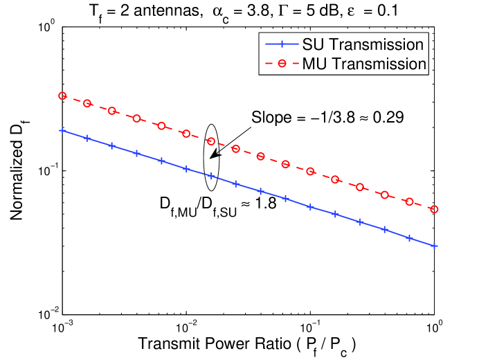
Figure 3: No-coverage femtocell radius for different values of $\frac{P_{f}}{P_{c}}$.

For fixed $T_{f}$, $U_{f}$ and $U_{c}$, the no-coverage femtocell radius $D_{f}$ in (5) scales as $(P_{f}/P_{c})^{-1/\alpha_{c}}$. Decreasing $D_{f}$ by a factor of $k$ requires increasing $P_{f}$ by $10\alpha_{c}\log_{10}k$ decibels. This suggests that a graph of $D_{f}$ versus $P_{f}/P_{c}$ (see Fig. 3) is a straight line on a log-log scale with slope $-1/\alpha_{c}$.

Next, we derive the maximum obtainable spatial reuse from multiple antenna femtocells when they share spectrum with cellular transmissions. Mathematically, the maximum femtocell contention density satisfying (3) is expressed as

$$\lambda_{f}^{\ast}(D)=\mathop{\rm arg\,max}\lambda_{f}(D),\ \textrm{subject to }\mathbb{P}{(\mathrm{SIR}_{f}(F_{0},D)\geq\Gamma)}\geq 1-\epsilon.$$ (9)

Theorem 2

In a two-tier network, the maximum femtocell contention density $\lambda_{f}^{\ast}(D)$ at distance $D$ from the macrocell $B_{0}$, which satisfies (9) (in the small-$\epsilon$ regime) is given as

$$\lambda_{f}^{\ast}(D)=\frac{1}{\mathcal{C}_{f}(\mathcal{Q}_{f}\Gamma)^{\delta_{f}}}\left[\frac{\epsilon-\mathcal{I}_{\frac{\kappa}{\kappa+1}}(T_{f}-U_{f}+1,U_{c})}{\frac{1}{\mathcal{K}_{f}}-\mathcal{I}_{\frac{\kappa}{\kappa+1}}(T_{f}-U_{f}+1,U_{c})}\right]$$ (10)

where $\delta_{f}=2/\alpha_{fo}$, $\mathcal{Q}_{f}$ is given by (2), $\kappa$ is given by (4), and

$$\mathcal{C}_{f}=\pi\delta_{f}U_{f}^{-\delta_{f}}\sum_{k=0}^{U_{f}-1}\binom{U_{f}}{k}B(k+\delta_{f},U_{f}-k-\delta_{f})$$ (11)

$$\mathcal{K}_{f}=\left[1+\frac{1}{(1+\kappa)^{U_{c}}}\sum_{j=0}^{T_{f}-U_{f}-1}\left(\frac{\kappa}{\kappa+1}\right)^{j}\binom{U_{c}+j-1}{j}\sum_{l=1}^{T_{f}-U_{f}-j}\frac{1}{l!}\prod_{m=0}^{(l-1)}(m-\delta_{f})\right]^{-1}$$ (12)

where $B(a,b)=\frac{\mathbf{\Gamma}(a)\mathbf{\Gamma}(b)}{\mathbf{\Gamma}(a+b)}$ denotes the Beta function and $\mathcal{K}_{f}=1$ whenever $U_{f}=T_{f}$.

Proof:

Refer to Appendix B ∎

Theorem 2 provides the maximum femtocell contention density at $D$ considering both cross-tier cellular and hotspot interference from neighboring femtocells. Alternatively, given an average of $\lambda_{f}$ transmitting femtocells per square meter, (10) can be inverted (numerically) to obtain the minimum $D$ which guarantees that (9) is feasible. Theorem 2 provides two fundamental operational regimes depending on the hotspot location relative to the macrocell.

Cellular-limited regime.

Assuming $\epsilon<\frac{1}{\mathcal{K}_{f}}$, a necessary condition for $\lambda_{f}^{\ast}(D)\geq 0$ in (10) is $\mathcal{I}_{\frac{\kappa}{\kappa+1}}(T_{f}-U_{f}+1,U_{c})\leq\epsilon$, or $\kappa(D)$ in (4) is upper bounded as

$$\kappa\leq\frac{\mathcal{I}^{-1}(\epsilon,T_{f}-U_{f}+1,U_{c})}{1-\mathcal{I}^{-1}(\epsilon,T_{f}-U_{f}+1,U_{c})}.$$

Indeed, from Theorem 1, a femtocell cannot guarantee reliable coverage to its users because of excessive cross-tier interference, whenever the above condition is violated.

Hotspot-limited regime.

As $\kappa\rightarrow 0$ or $D^{-\alpha_{c}}\rightarrow 0$, the SIR at any femtocell located at $D$ is primarily influenced by hotspot interference. Consequently, $\lambda_{f}^{\ast}(D)$ in (10) approaches the limit $\breve{\lambda}_{f}$ given as

$$\breve{\lambda}_{f}=\lim_{\kappa\rightarrow 0}\lambda_{f}^{\ast}(D)=\frac{\epsilon\ \breve{\mathcal{K}}_{f}}{\mathcal{C}_{f}(\mathcal{Q}_{f}\Gamma)^{\delta_{f}}}\ \textrm{, where }\breve{\mathcal{K}}_{f}=\lim_{\kappa\rightarrow 0}\mathcal{K}_{f}=\left[1+\sum_{l=1}^{T_{f}-U_{f}}\frac{1}{l!}\prod_{m=0}^{l-1}(m-\delta_{f})\right]^{-1}.$$ (13)

The limit $\breve{\mathcal{K}}_{f}$ determines the maximum contention density in the special case of an ad hoc network – no cellular interference – of homogeneously distributed transmitters equipped with multiple antennas [13]. Their work shows that $\breve{\mathcal{K}}_{f}$ and $\mathcal{C}_{f}$ scales with $T_{f}$ and $U_{f}$ as

$$\breve{\mathcal{K}}_{f}\sim\Theta[(T_{f}-U_{f}+1)^{\delta_{f}}],\ \mathcal{C}_{f}\mathcal{Q}_{f}^{\delta_{f}}\sim\Theta(U_{f}^{\delta_{f}}).$$ (14)

Further, $\forall\kappa\geq 0,\mathcal{K}_{f}\leq\breve{\mathcal{K}}_{f}$ and $\mathcal{K}_{f}$ is bounded as $(T_{f}-U_{f}+1)^{\delta_{f}}\leq\breve{\mathcal{K}}_{f}\leq\breve{\mathcal{K}}_{f,\textrm{max}}=\mathbf{\Gamma}(1-\delta_{f})(T_{f}-U_{f}+1)^{\delta_{f}}$ [13]. We shall now consider two cases in the hotspot-limited regime ($D^{-\alpha_{c}}\rightarrow 0$). First, with multiuser transmission to $U_{f}=T_{f}$ femtocell users and using (14), the femtocell area spectral efficiency (in $\mathrm{b/s/Hz/m^{2}}$) which is given as $(1-\epsilon)U_{f}\breve{\lambda}_{f}\log_{2}(1+\Gamma)$ scales according to $\Theta(T_{f}^{1-\delta_{f}})$. With SU transmission, the ASE scales as $\Theta(T_{f}^{\delta_{f}})$. This suggests that in path loss regimes with $\alpha_{fo}<4$, higher spatial reuse is obtainable (order-wise) provided femtocells employ their antennas to transmit to just one user. In contrast, MU femtocell transmission provides higher network-wide spatial reuse (order-wise) only when hotspot interference is significantly diminished ($\alpha_{fo}>4$).

III-B SIR Analysis at a Cellular User

We now consider a reference cellular user $0$ at distance $D$ from their macrocell $B_{0}$. During a given signaling interval, neglecting background noise, the received signal at user $0$ is then given as

$$y_{0}=\sqrt{A_{c}}D^{-\frac{\alpha_{c}}{2}}\mathbf{h}_{0}^{\dagger}\mathbf{V}\mathbf{s}+\sqrt{{A}_{c,f}}\sum_{F_{j}\in\Pi_{f}}\mathbf{e}_{j}^{\dagger}\mathbf{W}_{j}\mathbf{r}_{j}|X_{j}|^{-\frac{\alpha_{fo}}{2}}$$ (15)

where $\mathbf{s}\in\mathbb{C}^{U_{c}\times 1},\mathbb{E}[||\mathbf{s}||^{2}]\leq P_{c}$ and $\mathbf{r}_{j}\in\mathbf{C}^{U_{f}\times 1},\mathbb{E}[||\mathbf{r}_{j}||^{2}]\leq P_{f}$ represent the transmit data symbols for users in each tier. Further, $|X_{j}|$ and $\mathbf{e}_{j}\in\mathbb{C}^{T_{c}\times 1}$ respectively denote the distance and the downlink vector channel from the interfering femtocell $F_{j}$ to user $0$. The received SIR for user $0$ is given as

$$\mathrm{SIR}_{c}(B_{0},D)=\frac{\frac{P_{c}}{U_{c}}A_{c}D^{-\alpha_{c}}|\mathbf{h}_{0}^{\dagger}\mathbf{v}_{0}|^{2}}{\frac{P_{f}}{U_{f}}A_{c,f}\sum_{F_{j}\in\Pi_{f}}||\mathbf{e}_{j}^{\dagger}\mathbf{W}_{j}||^{2}|X_{j}|^{-\alpha_{fo}}}.$$ (16)

For successfully decoding user $0$’s signal, $\mathrm{SIR}_{c}(B_{0},D)$ should be greater than equal to the minimum SIR target $\Gamma$. Define $\mathcal{Q}_{c}=U_{c}\frac{P_{f}}{P_{c}}\frac{A_{c,f}}{A_{c}}D^{\alpha_{c}}$. Then, the probability of successful reception at $0$ is given as

$$\mathbb{P}{[\mathrm{SIR}_{c}(B_{0},D)\geq\Gamma]}=\mathbb{P}{\left[\frac{|\mathbf{h}_{0}^{\dagger}\mathbf{v}_{0}|^{2}}{\frac{1}{U_{f}}\sum_{F_{j}\in\Pi_{f}}||\mathbf{e}_{j}^{\dagger}\mathbf{W}_{j}||^{2}|X_{j}|^{-\alpha_{fo}}}\geq\mathcal{Q}_{c}\Gamma\right]}.$$ (17)

Both the desired channel powers denoted as $|\mathbf{h}_{0}^{\dagger}\mathbf{v}_{0}|^{2}$ and the interfering marks [19] given by $||\mathbf{e}_{j}^{\dagger}\mathbf{W}_{j}||^{2}$ follow a chi-squared distribution with $2(T_{c}-U_{c}+1)$ and $2U_{f}$ degrees of freedom respectively. Using [13], the maximum femtocell contention density $\lambda_{f}(D)$ for which (17) satisfies the maximum outage probability constraint $\mathbb{P}{(\mathrm{SIR}_{c}(B_{0},D)\geq\Gamma)}\geq 1-\epsilon$ of a cellular user is given as

$$\lambda_{f}^{\ast}(D)=\frac{\epsilon\mathcal{K}_{c}}{\mathcal{C}_{f}(\mathcal{Q}_{c}\Gamma)^{\delta_{f}}}\textrm{, where }\mathcal{K}_{c}=\left[1+\sum_{j=1}^{T_{c}-U_{c}}\frac{1}{j!}\prod_{k=0}^{j-1}(k-\delta_{f})\right]^{-1}$$ (18)

where $\delta_{f}=2/\alpha_{fo}$ as before and $\mathcal{C}_{f}$ is given by (11). From [13], $\mathcal{K}_{c}$ is bounded as

$$(T_{c}-U_{c}+1)^{\delta_{f}}\leq\mathcal{K}_{c}\leq\mathbf{\Gamma}(1-\delta_{f})\ (T_{c}-U_{c}+1)^{\delta_{f}}$$ (19)

where the upper bound is a good approximation for $\mathcal{K}_{c}$; for example, with $T_{c}=4$, $U_{c}=1$ and $\alpha_{fo}=3.8$, the term $K_{c}$ equals $3.47$ while the upper bound equals $3.87$.

Remark 3

Since (18) varies as $\mathcal{K}_{c}/U_{c}^{\delta_{f}}$, approximating $\mathcal{K}_{c}$ by the upper bound in (19) shows that the maximum contention density for single user beamforming given as $\lambda_{f,\textrm{SU}}^{\ast}(D)$ is proportional to $\mathbf{\Gamma}(1-\delta_{f})T_{c}^{\delta_{f}}$. With $1<U_{c}<T_{c}$ transmitted users, the maximum femtocell contention density denoted as $\lambda_{f,\textrm{MU}}^{\ast}(D)$ is proportional to $\mathbf{\Gamma}(1-\delta_{f})(T_{c}-U_{c}+1)^{\delta_{f}}/U_{c}^{\delta_{f}}$. Therefore, SU transmission increases the maximum hotspot density by a factor of $\left[T_{c}U_{c}/(T_{c}-U_{c}+1)\right]^{\delta_{f}}$. With $U_{c}=T_{c}$ users (implying $\mathcal{K}_{c}=1$), one obtains $\lambda_{f,\textrm{MU}}^{\ast}(D)$ to be proportional to $T_{c}^{-\delta_{f}}$, so that $\lambda_{f,\textrm{SU}}^{\ast}(D)/\lambda_{f,\textrm{MU}}^{\ast}(D)$ equals $\mathbf{\Gamma}(1-\delta_{f})T_{c}^{2\delta_{f}}$.

Given an average of $\lambda_{f}$ femtocells per sq. meter, inverting (18) yields the maximum distance up to which the cellular outage probability lies below $\epsilon$. This cellular coverage radius $D_{c}$ is given as

$$D_{c}=\left(\frac{1}{\Gamma U_{c}}\frac{A_{c}}{A_{c,f}}\frac{P_{c}}{P_{f}}\right)^{1/\alpha_{c}}\left({\frac{\epsilon\mathcal{K}_{c}}{\lambda_{f}\mathcal{C}_{f}}}\right)^{\frac{1}{\delta_{f}\alpha_{c}}}.$$ (20)

Remark 4

Since $D_{c}$ varies as $\left(P_{c}/P_{f}\right)^{1/\alpha_{c}}$, increasing the cellular coverage radius by a factor of $k$ necessitates increasing $P_{c}$ by $10\alpha_{c}\log_{10}k$ decibels relative to $P_{f}$.

Remark 5

In (20), $D_{c}$ is proportional to $(\frac{\mathcal{K}_{c}^{1/\delta_{f}}}{U_{c}})^{\frac{1}{\alpha_{c}}}$. With SU transmission [resp. MU transmission to $U_{c}=T_{c}$ users] at the macrocell and applying (19), the cellular coverage distance $D_{c}$ scales with $T_{c}$ as $D_{c,\textrm{SU}}\sim\Theta(T_{c}^{1/\alpha_{c}}),\ D_{c,\textrm{MU}}\sim\Theta(T_{c}^{-1/\alpha_{c}})$. This suggests that SU macrocell transmission provides coverage improvement by a factor of $T_{c}^{2/\alpha_{c}}$ (order-wise) relative to MU transmission.

III-C Design Interpretations

In this section, we provide design interpretations of the preceding results derived in Sections III-A and III-B in realistic path loss scenarios. We shall use the system parameters given in Table I and the path loss model described in Section II-A.

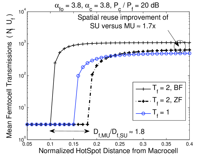
Figure 4: Maximum number of simultaneous femtocell transmissions $N_{f}U_{f}$ for different number of antennas and single-user versus multiple-user transmission per femtocell.

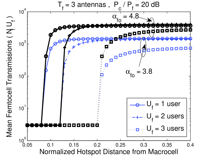
Figure 5: Maximum number of simultaneous femtocell transmissions $N_{f}U_{f}$ for different values of $\alpha_{fo}$.

Fig. 3 plots the normalized no-coverage femtocell radius $D_{f}$ versus $P_{f}/P_{c}$ on a log-log scale. Assuming a reference femtocell placed at distance $D$ w.r.t the macrocell BS, Figs. 4-5 plot the maximum number of simultaneous femtocell transmissions given as $N_{f}(D)U_{f}$ where $N_{f}(D)=\pi R_{c}^{2}\lambda_{f}^{\ast}(D)$, considering SU and MU femtocell transmissions and different values of $\alpha_{fo}$. Shown below are the three key observations.

Coverage improvement.

In the cellular-limited regime with $T_{f}=2$ antennas, Fig. 4 shows that SU transmission obtains a nearly $1.5$x reduction in the no-coverage femtocell radius $D_{f}$ w.r.t single antenna transmission. Next, both Figs. 3-4 show that SU transmission reduces $D_{f}$ by a factor of nearly $1.8$x relative to MU transmission. Both these observations agree with the predicted improvements in Corollary 1. This indicates that SU transmission significantly improves hotspot coverage.

Dominance of cellular interference.

In Figs. 4-5, $N_{f}$ increases from zero (at the no-coverage femtocell radius) to greater than $100$ femtocells per cell-site within a few meters outside the no-coverage radius. This step-like transition from the cellular-limited to the hot-spot limited regime suggests that cross-tier cellular interference is the capacity-limiting factor even in densely populated femtocell networks and interference between femtocells is negligible because of the proximity of home users to their APs and double wall partition losses.

Spatial reuse.

In the hotspot-limited regime with $\alpha_{fo}=3.8$, SU transmission consistently outperforms MU transmission. For example, with $T_{f}=2$ antennas, there is a nearly $1.7$x spatial reuse gain ($N_{f}U_{f}=1080$ with SU transmission versus $N_{f}U_{f}=640$ with MU transmission). In a scenario in which hotspot interference is significantly diminished (Fig. 5 with $\alpha_{fo}=4.8$ and $T_{f}=3$ antennas), MU transmission to $U_{f}=2$ hotspot users provides a marginally higher spatial reuse relative to SU transmission. The conclusion is that achieving the multiplexing benefits of MU transmission requires relative isolation (or large $\alpha_{fo}$) between actively transmitting femtocell APs.

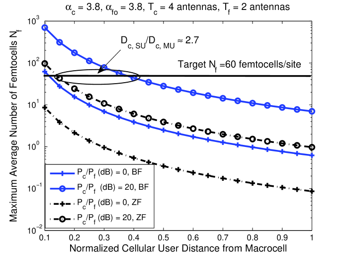
Figure 6: Maximum number of simultaneous femtocell transmissions satisfying outage probability constraint $\epsilon$ for a cellular user at different distances from the macrocell.

Fig. 6 plots the maximum number of transmitting femtocells $N_{f}=\pi R_{c}^{2}\ \lambda_{f}^{\ast}(D)$ as a function of the cellular user distance $D$. With $\left(P_{c}/P_{f}\right)_{\textrm{dB}}=20$ and a desired $N_{f}=60$ femtocells/cellsite, SU macrocell transmission provides a normalized cellular coverage radius $D_{c}\approx 0.35$. In contrast, the coverage provided by MU transmission is only $D_{c}\approx 0.13$, resulting in a coverage loss of $2.7$x relative to SU transmission (Remark 5 gives an order-wise loss of $\Theta(T_{c}^{\delta_{f}})=2.07$). With SU transmission and $(P_{c}/P_{f})_{\textrm{dB}}=0$, a cellular user at $D=0.1$ can tolerate interference from nearly $N_{f}=62$ femtocells/cellsite. In contrast, with MU transmission, $N_{f}$ reduces to nearly $8$ femtocells/cellsite. The observed improvement in the maximum femtocell contention density (equaling $7.75$x) is well approximated by the predicted improvement ($\mathbf{\Gamma}(1-\delta_{f})T_{c}^{2\delta_{f}}=8.04$x) in Remark 3.

The preceding observations reveal 1. since MU performance is significantly limited by residual hotspot interference, the macrocell should maximize cellular coverage by transmitting to just a single cellular user and 2. that femtocells should adapt their transmit powers depending on their location in order to ensure reliable cellular coverage .

IV Interference Management using Carrier-Sensing at Femtocells

To motivate carrier-sensing at femtocells, Fig. 4 shows that even with $(P_{c}/P_{f})_{\textrm{dB}}=20$, a femtocell at normalized distance $D=0.4$ can tolerate hotspot interference from greater than $1000$ neighboring femtocells. This suggests that in dense femtocell deployments, $(P_{c}/P_{f})_{\textrm{dB}}$ can be increased to minimize hotspot interference without violating the QoS requirement at femtocells. This section presents a carrier-sensing interference management strategy for choosing the femtocell transmission power provided there is a cellular user in its vicinity.

AS 3

Each cellular user periodically transmits over a set of uplink pilot slots (time or frequency resource) with power $P_{\textrm{UT,pilot}}$ for communicating their channel information to the macrocell.

AS 4

Each femtocell is capable of inferring its distance from its closest macrocell BS (either through GPS or measuring the average received power of the macrocell BS transmission, with prior calibration).

During carrier-sensing, each femtocell performs energy detection while monitoring uplink pilot cellular transmissions. In the absence of a cellular user, the femtocell maintains a constant transmit power $P_{f}$. When the detected energy of a cellular user exceeds a threshold, the femtocell chooses its $P_{f}$ based on its location $D$ within the underlying macrocell.

IV-A Minimum Required Sensing Range and Per-Tier Transmit Power Ratio Bounds

We shall first derive the minimum required sensing distance $D_{\textrm{sense}}$ such that any transmitting femtocell located within $R<D_{\textrm{sense}}$ meters of the cellular user violates its maximum outage probability requirement. Define the notation $\mathcal{B}(D_{\textrm{sense}})$ to denote a circular region of radius $D_{\textrm{sense}}$ containing $|\mathcal{B}(D_{\textrm{sense}})|$ femtocells. Given an intensity of $\lambda_{f}$ femtocells per square meter and assuming the cellular user $0$ is located at normalized distance $D$ w.r.t the macrocell, its outage probability is lower bounded as

$$\mathbb{P}[\mathrm{SIR}_{c}(B_{0},D)\leq\Gamma] \overset{(a)}{\geq}\mathbb{P}[\mathrm{SIR}_{c}(B_{0},D)\leq\Gamma,|\mathcal{B}(D_{\textrm{sense}})|>0]$$ (21)

$$\overset{(b)}{=}\mathbb{P}\left[\mathrm{SIR}_{c}(B_{0},D)\leq\Gamma\Big{|}|\mathcal{B}(D_{\textrm{sense}})|>0\right]\cdot(1-e^{-\lambda_{f}\pi D_{\textrm{sense}}^{2}})$$

$$\overset{(c)}{>}\mathbb{P}\left[\mathrm{SIR}_{c}(B_{0},D)\leq\Gamma\Big{|}|\mathcal{B}(D_{\textrm{sense}})|=1,R=D_{\textrm{sense}}\right]\cdot(1-e^{-\lambda_{f}\pi D_{\textrm{sense}}^{2}})$$

where step (a) in (21) is a lower bound as it ignores the event of zero hotspots present within $\mathcal{B}(D_{\textrm{sense}})$. Step (b) rewrites (a) in terms of the conditional probability. Finally, step (c) is a lower bound because it considers the event that $|\mathcal{B}(D_{\textrm{sense}})|=1$ and the hotspot is located exactly at $R=D_{\textrm{sense}}$ meters (thereby experiencing the highest path loss). A necessary condition for ensuring $\mathbb{P}[\mathrm{SIR}_{c}(B_{0},D)\leq\Gamma]\leq\epsilon$ is that the right hand side in step (c) in (21) consisting of the product of two probabilities should be less than $\epsilon$. The first term represents the outage probability from interfering hotspots due to the time-varying channel powers and the second term represents the probability that $\mathcal{B}(D_{\textrm{sense}})$ is non-empty.

Assuming large $\lambda_{f}$ (or $1-e^{-\lambda_{f}\pi D_{\textrm{sense}}^{2}}\rightarrow 1$), a reasonable choice for selecting $D_{\textrm{sense}}$ is to set the conditional outage probability $\mathbb{P}\left[\mathrm{SIR}_{c}(B_{0},D)\leq\Gamma\Big{|}|\mathcal{B}(D_{\textrm{sense}})|=1,R=D_{\textrm{sense}}\right]$, given exactly one interfering femtocell AP $F_{0}$ at distance $D_{\textrm{sense}}$ from the cellular user, to equal $\epsilon$. Evaluating this probability,

$$\mathbb{P}\left[\frac{\frac{P_{c}}{U_{c}}A_{c}D^{-\alpha_{c}}|\mathbf{h}_{0}^{\dagger}\mathbf{v}_{0}|^{2}}{\frac{P_{f}}{U_{f}}A_{c,f}||\mathbf{e}_{0}^{\dagger}\mathbf{W}_{0}||^{2}D_{\textrm{sense}}^{-\alpha_{fo}}}\leq\Gamma\right] =\mathbb{P}\left[\frac{|\mathbf{h}_{0}^{\dagger}\mathbf{v}_{0}|^{2}}{||\mathbf{e}_{0}^{\dagger}\mathbf{W}_{0}||^{2}}\leq\frac{\Gamma\mathcal{Q}_{c}D_{\textrm{sense}}^{-\alpha_{fo}}}{U_{f}}\right]$$ (22)

$$\overset{(a)}{=}\mathbb{P}\left[Z\leq\theta\frac{U_{f}}{T_{c}-U_{c}+1}\right]$$

$$\overset{(b)}{=}\mathcal{I}_{\frac{\theta}{\theta+1}}(T_{c}-U_{c}+1,U_{f})$$

where $\mathcal{Q}_{c}=U_{c}\frac{P_{f}}{P_{c}}\frac{A_{c,f}}{A_{c}}D^{\alpha_{c}}$ as before, while the terms $|\mathbf{h}_{0}^{\dagger}\mathbf{v}_{0}|^{2}\sim\chi^{2}_{2(T_{c}-U_{c}+1)}$ and $||\mathbf{e}_{0}^{\dagger}\mathbf{W}_{0}||^{2}\sim\chi^{2}_{2U_{f}}$ denote the chi-squared distributed desired and interfering channel powers, as given earlier in (17). Step (a) in (22) follows by defining $\theta\triangleq\mathcal{Q}_{c}\Gamma D_{\textrm{sense}}^{-\alpha_{fo}}/U_{f}$ and defining the normalized ratio $Z=\frac{|\mathbf{h}_{0}^{\dagger}\mathbf{v}_{0}|^{2}/(T_{c}-U_{c}+1)}{||\mathbf{e}_{0}^{\dagger}\mathbf{W}_{0}||^{2}/U_{f}}$ which is F-distributed [26]. Step (b) follows by substituting the cdf of the F-distributed r.v $Z$. The minimum required sensing radius at $D$ is consequently given as

$$D_{\textrm{sense}}\geq\left[\left(\frac{\mathcal{Q}_{c}\Gamma}{U_{f}}\right)\left(\frac{1-\mathcal{I}^{-1}(\epsilon;T_{c}-U_{c}+1,U_{f})}{\mathcal{I}^{-1}(\epsilon;T_{c}-U_{c}+1,U_{f})}\right)\right]^{1/\alpha_{fo}}.$$ (23)

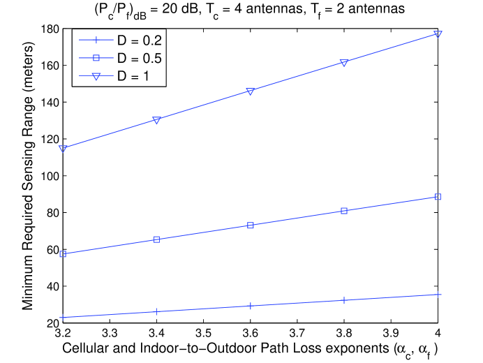
Figure 8: Necessary sensing range (in meters) per femtocell (assuming SU transmission in each tier) as a function of the path loss exponents $\alpha_{c},\alpha_{f}$ and the normalized distance $D$ of the cellular user.

Using the numerical values in Table I, Fig. 8 plots $D_{\textrm{sense}}$ for different values of the path loss exponents $\alpha_{c}$ and $\alpha_{fo}$ as well as different cellular user locations $D$. Assuming SU transmission in both tiers, $(P_{c}/P_{f})_{\textrm{dB}}=20$ dB and $\alpha_{c}=\alpha_{fo}=3.8$, a minimum sensing range $D_{\textrm{sense}}\approx 160$ meters is required at the cell-edge ($D=R_{c}$).

Next, the following lemma derives bounds on $P_{c}/P_{f}$ that satisfy the per-tier outage probability requirements at distance $D$ from the macrocell.

Lemma 1

Given a mean intensity of $\lambda_{f}$ femtocells per square meter and minimum per-tier SIR target $\Gamma$, satisfying the per-tier outage probability requirement at distance $D$ from the macrocell necessitates $(P_{c}/P_{f})$ to be bounded as $(P_{c}/P_{f})_{\textrm{lb}}[D]\leq P_{c}/P_{f}\leq(P_{c}/P_{f})_{\textrm{ub}}[D]$, which are given as

$$\left(\frac{P_{c}}{P_{f}}\right)_{\textrm{lb}}[D] =\Gamma\left(\frac{A_{c,f}}{A_{c}}\right)\left(\frac{U_{c}}{D^{-\alpha_{c}}}\right)\left(\frac{\mathcal{C}_{f}\lambda_{f}}{\epsilon\mathcal{K}_{c}}\right)^{1/\delta_{f}}$$ (24)

$$\left(\frac{P_{c}}{P_{f}}\right)_{\textrm{ub}}[D] =\left(\frac{1}{\Gamma}\right)\left(\frac{A_{fi}}{A_{f,c}}\right)\left(\frac{U_{c}R_{f}^{-\alpha_{fi}}}{U_{f}D^{-\alpha_{c}}}\right)\frac{\mathcal{I}^{-1}(\tilde{\epsilon};T_{f}-U_{f}+1,U_{c})}{1-\mathcal{I}^{-1}(\tilde{\epsilon};T_{f}-U_{f}+1,U_{c})}$$ (25)

where $\delta_{f}=2/\alpha_{fo}$ as before, $\mathcal{K}_{c}$ is given by (18), $\mathcal{Q}_{f}$ is given by (2), $\mathcal{C}_{f}$ is given by (11) and

$$\tilde{\epsilon}=\frac{\epsilon-\lambda_{f}\mathcal{C}_{f}(\mathcal{Q}_{f}\Gamma_{f})^{\delta_{f}}/\breve{\mathcal{K}}_{f,\textrm{max}}}{1-\lambda_{f}\mathcal{C}_{f}(\mathcal{Q}_{f}\Gamma_{f})^{\delta_{f}}}\textrm{ and }\breve{\mathcal{K}}_{f,\textrm{max}}=(T_{f}-U_{f}+1)^{\delta_{f}}\mathbf{\Gamma}(1-\delta_{f}).$$ (26)

Proof:

A lower limit on $P_{c}/P_{f}$ is obtained by computing the minimum $P_{c}$ required to satisfy the outage probability requirement for a cellular user at distance $D$ w.r.t $B_{0}$. Combining (18) and (19) yields $(P_{c}/P_{f})_{\textrm{lb}}$ in (24). Conversely, given a femtocell user at distance $D$ w.r.t $B_{0}$, an upper limit for $P_{c}/P_{f}$ is obtained by computing the minimum required $P_{f}$ for satisfying $\mathbb{P}[\textrm{SIR}(F_{0},D)\leq\Gamma]\leq\epsilon$. Substituting the upper bound for $\mathcal{K}_{f}$ and inverting (10) to compute $(P_{c}/P_{f})_{\textrm{ub}}$ yields (25). ∎

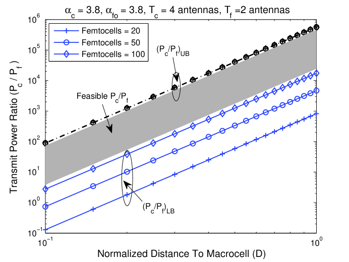
Figure 7: Lower and upper bounds on $P_{c}/P_{f}$ with SU transmission as a function of the distance $D$. Shaded region shows feasible $P_{c}/P_{f}$’s at location $D$, which satisfies the per-tier outage probability requirement for different average numbers of femtocells per cell-site.

Inspecting (24) and (25) reveals that the difference between the decibel upper and lower bounds is constant for all $D$. Fig. 7 plots $(P_{c}/P_{f})_{\textrm{lb}}$ and $(P_{c}/P_{f})_{\textrm{ub}}$ for different normalized $D$. At a cell-edge ($D=1$) location, the bounds on the required $(P_{c}/P_{f})_{\textrm{dB}}$ are given as $40\leq(P_{c}/P_{f})_{\textrm{dB}}\leq 55$ dB.

IV-B Energy Detection based Carrier-Sensing of Cellular Users

Assume that each femtocell monitors a set of pilot slots (we assume time-slotted transmission in the subsequent discussion) and employs energy detection[27]. We briefly describe the sensing procedure below and refer to [27, 28, 17, 14] for further details.

Let $T$ denote the sensing time (number of sensing time slots times the slot duration) and $W$ designate the sensed bandwidth. Given a received signal $x(t)$ in the pilot slots and $n(t)$ being complex Gaussian noise process with power $N_{0}W/2$ per complex dimension, define the following hypotheses namely 1. $\mathcal{H}_{0}$: Absence of cellular user [$x(t)=n(t)$] and 2. $\mathcal{H}_{1}$: Presence of an active cellular user [$x(t)=hs(t)+n(t)$]. The femtocell compares the energy detector output $Y=2/N_{0}\int_{0}^{T}|x(t)|^{2}\textrm{ d}t$ against a threshold $\lambda$ for inferring the presence (or absence) of a cellular user. Define $m$ to equal the time-bandwidth product $TW$ (assumed to be an integer). The average sensed pilot Signal-to-Noise Ratio (SNR) at the femtocell is given as

$$\overline{\gamma}=\frac{P_{\textrm{UT,pilot}}D^{-\alpha_{c}}A_{f,c}}{N_{0}W}\textrm{, where }(N_{0}W)_{\textrm{dB}}=P_{c,\textrm{dB}}-A_{c,\textrm{dB}}-10\alpha_{c}\log_{10}(R_{c})-\overline{\gamma}_{\textrm{edge,dB}}$$ (27)

where $D$ denotes the distance of the cellular user from the femtocell. The noise power $N_{0}W$ is chosen with reference to a cell-edge user obtaining an average downlink SNR $\overline{\gamma}_{\textrm{edge}}>\Gamma$. Assuming Selection Combining (SC) is used at the $T_{f}$ available diversity branches for choosing the maximum SNR branch, the detection probability $P_{\textrm{detect,SC}}$ and the false-alarm probability $P_{\textrm{false}}$ are respectively given as [28, 17]

$$P_{\textrm{detect,SC}}=\mathbb{P}[Y>\lambda|\mathcal{H}_{1}] =T_{f}\cdot\sum_{i=0}^{T_{f}-1}\frac{(-1)^{i}}{i+1}\binom{T_{f}-1}{i}P_{d,\textrm{Ray}}\left(\frac{\overline{\gamma}}{i+1}\right),P_{\textrm{false}}=\mathbb{P}[Y>\lambda|\mathcal{H}_{0}]=\frac{\mathbf{\Gamma}(2m,\lambda)}{\mathbf{\Gamma}(2m)}$$

$$\textrm{where }P_{\textrm{detect,Ray}}(\overline{\gamma}) =\frac{\mathbf{\Gamma}(2m-1,\lambda)}{\mathbf{\Gamma}(2m-1)}+e^{-\frac{\lambda}{(1+m\overline{\gamma})}}\left(1+\frac{1}{m\overline{\gamma}}\right)^{2m-1}\left[1-\frac{\mathbf{\Gamma}(2m-1,\frac{\lambda m\overline{\gamma}}{(1+\lambda m\overline{\gamma})})}{\mathbf{\Gamma}(2m-1)}\right].$$ (28)

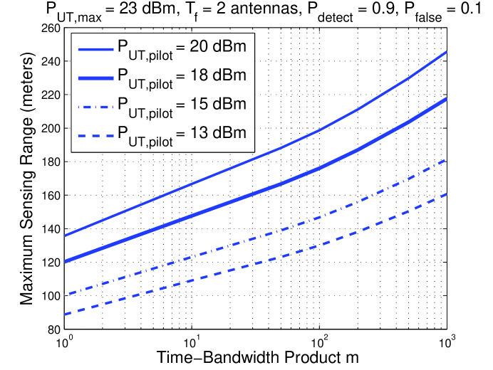
Figure 9: Maximum sensing range (in meters) at each femtocell as a function of the sensing time-bandwidth product and uplink pilot transmission powers.

Here, $\mathbf{\Gamma}(a,x)=\int_{x}^{\infty}t^{a-1}e^{-t}\textrm{d}t$ is the upper incomplete gamma function. Because of the complex baseband signal model, there is a factor of $2$ discrepancy in (IV-B) with respect to [17]. Fig. 9 plots the maximum femtocell sensing range $D_{\textrm{sense}}$ versus different values of the time-bandwidth product $m$. For example, with $P_{\textrm{UT,pilot}}=20$ dBm ($3$ dB below the maximum UT transmit power), and probabilities $P_{\textrm{detect}}=0.9$ and $P_{\textrm{false}}=0.1$ respectively, obtaining a sensing range of $D_{\textrm{sense}}=230$ meters requires a minimum time-bandwidth product $m=500$.

V Numerical Results

This section reports the results of computer simulations using the system parameters in Table I. The simulation consisted of $1000$ different random drops of femtocell hotspots with $1000$ trials per drop to simulate Rayleigh fading. Additive white Gaussian noise power was chosen to obtain an average cell-edge SNR of $\overline{\gamma}_{\textrm{edge, dB}}=12$ dB. Single-user transmission is assumed in either tier considering its superior coverage and spatial reuse performance. With an average of $N_{f}=60$ femtocells per cell-site, we evaluate whether the $10$ percentile outage capacity ($\epsilon=0.1$) satisfies the minimum required per-tier spectral efficiency $\log_{2}(1+\Gamma)$ b/s/Hz (or nearly $2.06$ b/s/Hz for $\Gamma_{\textrm{dB}}=5$).

During carrier-sensing, each femtocell can detect active cellular users within a sensing radius equaling $230$ meters (determined using computer simulations), which exceeds the minimum required sensing range of $D_{\textrm{sense}}=160$ meters obtained in Section IV-A. We consider both a fixed $P_{c}/P_{f}$ (without carrier-sensing or power control at femtocells) and a location based selection of $P_{c}/P_{f}$ (wherein femocells adjust their $P_{f}$ upon sensing a cellular user). Under ambient conditions (no detected cellular user), a fixed $(P_{c}/P_{f})_{\textrm{dB}}=20$ dB is chosen. Upon sensing a cellular user, a femtocell chooses its $P_{f}$ such that $(P_{c}/P_{f})[D,\textrm{dB}]=0.7(P_{c}/P_{f})_{\textrm{ub}}[D,\textrm{dB}]+0.3(P_{c}/P_{f})_{\textrm{lb}}[D,\textrm{dB}]$, which are given in (24)-(25). Two scenarios are considered namely

Reference Cellular User.

A cellular user is placed at normalized distances ($D=0.8$ and $D=1.0$) w.r.t the macrocell. The cdfs of the achievable cellular data rates have been reported.

Reference Hotspot.

A reference hotspot is placed at normalized distances ($D=0.11,0.4,0.6,0.8$ and $0.9$ respectively) from the macrocell. A reference cellular user is co-linearly placed at a distance $D_{\textrm{sense}}/2$ w.r.t the hotspot. The conditional cdfs of the hotspot data rates (assuming idealized sensing) have been reported.

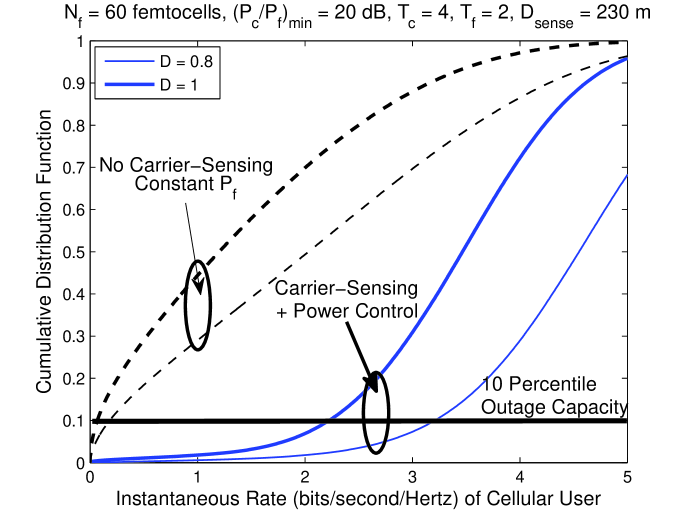
Figure 10: Cumulative distribution function of the instantaneous cellular data rate (in b/s/Hz) with SU transmission in each tier.

Fig. 10 shows the cdfs of the obtained cellular data rates for $N_{f}=60$ femtocells/cell-site. Without carrier-sensing, the $10$ percentile outage capacities are below $0.5$ b/s/Hz. By employing carrier-sensing, the $10$ percentile outage capacities (corresponding to $\epsilon=0.1$) equal $3.21$ b/s/Hz and $2.22$ b/s/Hz for cellular user locations of $D=0.8$ and $D=1.0$ respectively. Thus, our scheme ensures uniform cell-edge coverage with large numbers of femtocells.

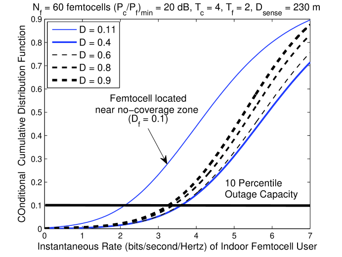
Figure 11: Conditional cumulative distribution function of a femtocell user’s data rate (in b/s/Hz) (conditioned on a carrier-sensed cellular user at distance $D_{\textrm{sense}}/2$). Single-user transmission is employed in each tier.

Fig. 11 shows the cdfs of the obtained femtocell data rates with carrier-sensing and transmit power control at femtocell APs. The lowest outage capacity is obtained when the femtocell is located close to the no-coverage zone ($D=0.11$). Because the location-based power control scheme monotonically decreases transmit power with femtocell distance from $B_{0}$, the outage capacities monotonically decrease with $D$. The $10$ percentile outage capacities are respectively equal to $2.15,3.63,3.56,3.32$ and $3.22$ b/s/Hz for the different femtocell locations given above which exceeds the minimum desired target spectral efficiency of $2.06$ b/s/Hz.

VI Conclusions

In two-tier cellular systems with universal frequency reuse, cross-tier interference will likely be the main obstacle preventing uniform coverage. This paper has derived analytical expressions for the coverage zones in such a tiered architecture with spatial diversity considering the number of antennas, the maximum tolerable outage probability accounting for path loss and Rayleigh fading. Single-user transmission in either tier is analytically shown to provide significantly superior coverage and spatial reuse while performance of multiple-user transmission suffers from residual cross-tier interference. For providing uniform cellular coverage, we have proposed a location-assisted power control scheme for regulating femtocell transmit powers. This scheme is fully decentralized and provides uniform cellular and hotspot coverage on the cell-edge, as opposed to randomized hotspot transmissions without carrier-sensing. These results motivate deploying closed-access tiered cellular architectures while requiring minimal network overhead.

Appendix A Proof of Theorem 1

The probability of successful reception in (3) can be upper bounded as

$$\mathbb{P}{[\mathrm{SIR}_{f}(F_{0},D)\geq\Gamma]}\leq\mathbb{P}{\left[|\mathbf{g}_{0}^{\dagger}\mathbf{w}_{0,0}|^{2}\geq\Gamma\mathcal{Q}_{f}\left(\frac{\mathcal{P}_{f}}{U_{c}}||\mathbf{f}_{0}^{\dagger}\mathbf{V}||^{2}\right)\right]}=\mathbb{P}{\left[|\mathbf{g}_{0}^{\dagger}\mathbf{w}_{0,0}|^{2}\geq\kappa||\mathbf{f}_{0}^{\dagger}\mathbf{V}||^{2}\right]}.$$ (29)

The term $|\mathbf{g}_{0}^{\dagger}\mathbf{w}_{0,0}|^{2}$ is distributed as a chi-squared random variable (r.v) $X$ with $2(T_{f}-U_{f}+1)$ degrees of freedom denoted as $\chi^{2}_{2(T_{f}-U_{f}+1)}$. To prove this claim, whenever $U_{f}=1$ (beamforming to a single user), $\mathbf{w}_{0,0}=\frac{\mathbf{g}_{0}}{\left|\left|\mathbf{g}_{0}\right|\right|}$, therefore, $|\mathbf{g}_{0}^{\dagger}\mathbf{w}_{0,0}|^{2}$ is distributed as $\chi^{2}_{2T_{f}}$. When $1<U_{f}\leq T_{f}$, $|\mathbf{g}_{0}^{\dagger}\mathbf{w}_{0,0}|^{2}=|\frac{\mathbf{g}_{0}^{\dagger}}{\left|\left|\mathbf{g}_{0}\right|\right|}\mathbf{w}_{0,0}|^{2}\cdot\left|\left|\mathbf{g}_{0}\right|\right|^{2}$ which equals the product of two independent r.v’s which are distributed as $\textrm{Beta}(T_{f}-U_{f}+1,U_{f}-1)$ (see [29, Theorem 1.1] for proof) and $\chi^{2}_{2T_{f}}$ respectively. In [30, Pages 169-170], it is shown that $|\mathbf{g}_{0}^{\dagger}\mathbf{w}_{0,0}|^{2}$ is distributed as a $\chi^{2}_{2(T_{f}-U_{f}+1)}$ r.v. The probability density function of $|\mathbf{g}_{0}^{\dagger}\mathbf{w}_{0,0}|^{2}$ is given as $f_{|\mathbf{g}_{0}^{\dagger}\mathbf{w}_{0,0}|^{2}}(x)=x^{T_{f}-U_{f}}e^{-x}/\mathbf{\Gamma}(T_{f}-U_{f}+1)\ \forall x\geq 0$ where $\mathbf{\Gamma}(k)=(k-1)!$ for any positive integer $k$. Similarly, the r.v $||\mathbf{f}_{0}^{\dagger}\mathbf{V}||^{2}=\sum_{k=0}^{U_{c}-1}|\mathbf{f}_{0}^{\dagger}\mathbf{v}_{k}|^{2}$ is the sum of $U_{c}$ r.v’s, wherein each term $|\mathbf{f}_{0}^{\dagger}\mathbf{v}_{k}|^{2}$ equals the squared modulus of a linear combination of $T_{c}$ complex normal r.v’s, which is exponentially distributed. Consequently, $||\mathbf{h}_{0,c}^{\dagger}\mathbf{V}||^{2}$ is distributed as a $\chi^{2}_{2U_{c}}$ r.v.

Define $Z=\frac{|\mathbf{g}_{0}^{\dagger}\mathbf{w}_{0,0}|^{2}}{||\mathbf{f}_{0}^{\dagger}\mathbf{V}||^{2}}$. Then $Z$ is the ratio of two independent $\chi^{2}$ r.v’s with $2(T_{f}-U_{f}+1)$ and $2U_{c}$ degrees of freedom respectively. Therefore, $Z$ follows a canonical $F_{c}$-distribution[26] and $\frac{Z\ U_{c}}{(T_{f}-U_{f}+1)}$ is an F-distributed r.v with parameters $2(T_{f}-U_{f}+1)$ and $2U_{c}$ respectively. Substituting $\kappa$ in (4) and taking the complement of (29), one obtains

$$\mathbb{P}{[\mathrm{SIR}_{f}(F_{0},D)\leq\Gamma]}\geq\mathbb{P}{[Z\leq\kappa]}=\mathbb{P}{\left[\frac{Z\ U_{c}}{T_{f}-U_{f}+1}\leq\kappa\frac{U_{c}}{T_{f}-U_{f}+1}\right]}=\mathcal{I}_{\frac{\kappa}{\kappa+1}}(T_{f}-U_{f}+1,U_{c}).$$

A necessary condition for meeting the QoS requirement $\epsilon$ for indoor users served by $F_{0}$ is given as

$$\mathcal{I}_{\frac{\kappa}{\kappa+1}}(T_{f}-U_{f}+1,U_{c})\leq\epsilon\Rightarrow\kappa^{\ast}=\frac{\mathcal{I}^{-1}(\epsilon;T_{f}-U_{f}+1,U_{c})}{1-\mathcal{I}^{-1}(\epsilon;T_{f}-U_{f}+1,U_{c})}.$$

Substituting the definition of $\kappa$ in (4), one obtains $D_{f}$. This completes the proof.

Appendix B

Using (3), the probability of successful reception $\mathbb{P}{[\mathrm{SIR}_{f}(F_{0},D)\geq\Gamma]}$ is given as

$$\mathbb{P}{[|\mathbf{g}_{0}^{\dagger}\mathbf{w}_{0,0}|^{2}\geq\Gamma\mathcal{Q}_{f}(I_{f,c}+I_{f,f})]}\textrm{, where }I_{f,c}=\frac{\mathcal{P}_{f}}{U_{c}}||\mathbf{f}_{0}^{\dagger}\mathbf{V}||^{2},\ I_{f,f}=1/U_{f}\sum_{F_{j}\in\Pi_{f}\setminus F_{0}}||\mathbf{g}_{0,j}^{\dagger}\mathbf{W}_{j}||^{2}|X_{0,j}|^{-\alpha_{fo}}.$$

The interference from neighboring femtocells $I_{f,f}$ is a Poisson Shot-noise Process ([31, 32]) with independent and identically distributed marks[19]. The distributions of the signal powers and marks of the interferers are chi-squared with degrees of freedom given as $|\mathbf{g}_{0}^{\dagger}\mathbf{w}_{0,0}|^{2}\sim\chi^{2}_{2(T_{f}-U_{f}+1)},\ ||\mathbf{f}_{0}^{\dagger}\mathbf{V}||^{2}\sim\chi^{2}_{2U_{c}}$ and $||\mathbf{g}_{0,j}^{\dagger}\mathbf{W}_{j}||^{2}\sim\chi^{2}_{2U_{f}}$ respectively. Consequently,

$$\mathbb{P}{[\mathrm{SIR}_{f}(F_{0},D)\geq\Gamma]} \overset{(a)}{=}\int_{0}^{\infty}\sum_{k=0}^{T_{f}-U_{f}}\frac{(s\mathcal{Q}_{f}\Gamma)^{k}}{k!}e^{-s\mathcal{Q}_{f}\Gamma}\textrm{d}\mathbb{P}{(I_{f,c}+I_{f,f}\leq s)}$$ (30)

$$\overset{(b)}{=}\sum_{k=0}^{T_{f}-U_{f}}\frac{(-\mathcal{Q}_{f}\Gamma)^{k}}{k!}\frac{\textrm{d}^{k}}{\textrm{d}\theta^{k}}\mathcal{L}_{I_{f,c}}(\theta)\mathcal{L}_{I_{f,f}}(\theta)\Big{\rvert}_{\theta=\mathcal{Q}_{f}\Gamma}$$ (31)

where step $(a)$ follows by conditioning on $I_{f,c}+I_{f,f}$ and computing the complementary cumulative distribution (ccdf) of $||\mathbf{g}_{0}||^{2}$. For deriving step $(b)$, with $k=0$, the integral in $(a)$ corresponds to the Laplace Transform (LT) of the r.v $I_{f,f}+I_{f,c}$ given as $\mathbb{E}[e^{-(I_{f,c}+I_{f,f})\theta}]$ evaluated at $\theta=\mathcal{Q}_{f}\Gamma$ (originally derived in [23]). Next, since $I_{f,c}$ and $I_{f,f}$ are independent r.v’s, the LT of their sum decouples as the product of their LTs $\mathbb{E}[e^{-I_{f,c}\theta}]\mathbb{E}[e^{-I_{f,f}\theta}]$. Finally, for any $k>0$, we have the identity $\mathcal{L}[t^{k}f(t)]=(-1)^{k}F^{(k)}(s)$, where $F^{k}(s)$ represents the $k$th derivative of $F(s)$ (this technique is borrowed from [13]).

The LTs of $I_{f,c}$ and $I_{f,f}$ may be written as

$$\mathcal{L}_{I_{f,c}}(\theta)=\mathbb{E}[e^{-\theta I_{f,c}}]=\frac{1}{(1+\mathcal{P}_{f}\theta/U_{c})^{U_{c}}}$$ (32)

$$\mathcal{L}_{I_{f,f}}(\theta)=\mathbb{E}[e^{-\theta I_{f,f}}] \overset{(a)}{=}\exp\left\{-\lambda_{f}\int_{\mathbb{R}^{2}}1-\mathbb{E}_{S}[e^{-\theta\frac{S}{U_{f}}|x|^{-\alpha_{fo}}}]\ \textrm{d}x\right\},\textrm{where }S\sim\chi^{2}_{2U_{f}}$$

$$\overset{(b)}{=}\exp\left\{-\pi\lambda_{f}\delta_{f}\left(\frac{\theta}{U_{f}}\right)^{\delta_{f}}\sum_{k=0}^{U_{f}-1}\binom{U_{f}}{k}B(k+\delta_{f},U_{f}-k-\delta_{f})\right\}$$

$$\overset{(c)}{=}\exp(-\lambda_{f}\mathcal{C}_{f}\theta^{\delta_{f}})$$ (33)

where (32) follows from the LT of a chi-squared r.v with $2U_{c}$ degrees of freedom. In (B), step $(a)$ represents the LT of a Poisson Shot-Noise process with independent and identically distributed marks $S_{j}$ – equaling $||\mathbf{g}_{0,j}^{\dagger}\mathbf{W}_{j}||^{2}$ in our case. Defining $\delta_{f}\triangleq\frac{2}{\alpha_{fo}}$, steps $(b)$ and $(c)$ follow from [13]. Substituting (32) and (B) in (31) leads to the following requirement for the success probability

$$\sum_{k=0}^{T_{f}-U_{f}}\frac{(-\mathcal{Q}_{f}\Gamma)^{k}}{k!}\frac{\textrm{d}^{k}}{\textrm{d}\theta^{k}}\frac{e^{-\lambda_{f}\mathcal{C}_{f}\theta^{\delta_{f}}}}{(1+\frac{\mathcal{P}_{f}\theta}{U_{c}})^{U_{c}}}\geq 1-\epsilon,\textrm{where }\theta=\mathcal{Q}_{f}\Gamma.$$ (34)

Using the Leibniz rule, the $k$th derivative of $\mathcal{L}_{I_{f,c}}(\theta)\mathcal{L}_{I_{f,f}}(\theta)$ is given as

$$\frac{\textrm{d}^{k}}{\textrm{d}\theta^{k}}\frac{e^{-\lambda_{f}\mathcal{C}_{f}\theta^{\delta_{f}}}}{(1+\frac{\mathcal{P}_{f}\theta}{U_{c}})^{U_{c}}}=\sum_{j=0}^{k}\binom{k}{j}\frac{\textrm{d}^{j}}{\textrm{d}\theta^{j}}\left(1+\frac{\mathcal{P}_{f}\theta}{U_{c}}\right)^{-U_{c}}\frac{\textrm{d}^{(k-j)}}{\textrm{d}\theta^{(k-j)}}e^{-\lambda_{f}\mathcal{C}_{f}\theta^{\delta_{f}}}.$$ (35)

where $\binom{a}{b}$ is the coefficient of $x^{b}$ in the expansion of $(1+x)^{a}$. Considering the low outage regime, we shall evaluate the $k$th derivative of $\mathcal{L}_{I_{f,f}}(\theta)$ using a first-order Taylor series approximation around $\lambda_{f}\mathcal{C}_{f}\theta^{\delta_{f}}=0$. Then, for all $k\geq 1$, the $k$th derivatives of $\mathcal{L}_{I_{f,c}}(\theta)$ and $\mathcal{L}_{I_{f,f}}(\theta)$ are individually given as

$$\frac{\textrm{d}^{k}}{\textrm{d}\theta^{k}}\left(1+\frac{\mathcal{P}_{f}\theta}{U_{c}}\right)^{-U_{c}}=\frac{\left[\prod_{j=0}^{k-1}(U_{c}+j)\right]\left(\frac{\mathcal{-P}_{f}}{U_{c}}\right)^{k}}{(1+\frac{\mathcal{P}_{f}\theta}{U_{c}})^{k+U_{c}}}.$$ (36)

$$\frac{\textrm{d}^{k}}{\textrm{d}\theta^{k}}e^{-\lambda_{f}\mathcal{C}_{f}\theta^{\delta_{f}}}=-\left[\lambda_{f}\mathcal{C}_{f}\prod_{m=0}^{k-1}(\delta_{f}-m)\theta^{\delta_{f}-k}\right]e^{-\lambda_{f}\mathcal{C}_{f}\theta^{\delta_{f}}}+\Theta(\lambda_{f}^{2}\mathcal{C}_{f}^{2}\theta^{2\delta_{f}}).$$ (37)

Combining (34) with (36) and (37) and substituting $\theta=\mathcal{Q}_{f}\Gamma$ leads to

$$\frac{e^{-\lambda_{f}\mathcal{C}_{f}(\mathcal{Q}_{f}\Gamma)^{\delta_{f}}}}{(1+\frac{\mathcal{P}_{f}\mathcal{Q}_{f}\Gamma}{U_{c}})^{U_{c}}}\Biggl{\{}\sum_{k=0}^{(T_{f}-U_{f})}\frac{(\frac{\mathcal{P}_{f}\mathcal{Q}_{f}\Gamma}{U_{c}})^{k}}{k!\left(1+\frac{\mathcal{P}_{f}\mathcal{Q}_{f}\Gamma}{U_{c}}\right)^{k}}\prod_{m=0}^{(k-1)}(U_{c}+m)$$

$$- \lambda_{f}\mathcal{C}_{f}(\mathcal{Q}_{f}\Gamma)^{\delta_{f}}\sum_{k=1}^{(T_{f}-U_{f})}\frac{(-1)^{k}}{k!}\sum_{j=1}^{k}\binom{k}{j}\left[\frac{\frac{-\mathcal{P}_{f}\mathcal{Q}_{f}\Gamma}{U_{c}}}{1+\frac{\mathcal{P}_{f}\mathcal{Q}_{f}\Gamma}{U_{c}}}\right]^{k-j}\prod_{n=0}^{(k-j-1)}(U_{c}+n)\prod_{m=0}^{j-1}(\delta_{f}-m)\Biggr{\}}$$

$$+ \Theta(\lambda_{f}^{2}\mathcal{C}_{f}^{2}(\mathcal{Q}_{f}\Gamma)^{2\delta_{f}})\geq 1-\epsilon.$$

Next, substituting $\kappa=\mathcal{P}_{f}\mathcal{Q}_{f}\Gamma/U_{c}$ from (4) and performing a first-order Taylor series expansion of $e^{-\lambda_{f}\mathcal{C}_{f}(\mathcal{Q}_{f}\Gamma)^{\delta_{f}}}=1-\lambda_{f}C_{f}(\mathcal{Q}_{f}\Gamma)^{\delta_{f}}+\Theta(\lambda_{f}^{2}\mathcal{C}_{f}^{2}(\mathcal{Q}_{f}\Gamma)^{2\delta_{f}})$, the above expression simplifies as

$$\frac{1-\lambda_{f}\mathcal{C}_{f}(\mathcal{Q}_{f}\Gamma)^{\delta_{f}}}{(1+\kappa)^{U_{c}}}\Biggl{\{}\sum_{k=0}^{T_{f}-U_{f}}\frac{1}{k!}\left(\frac{\kappa}{\kappa+1}\right)^{k}\prod_{m=0}^{k-1}(U_{c}+m)$$ (38)

$$- \lambda_{f}\mathcal{C}_{f}(\mathcal{Q}_{f}\Gamma)^{\delta_{f}}\sum_{k=1}^{T_{f}-U_{f}}\frac{1}{k!}\sum_{j=1}^{k}\binom{k}{j}\left[\frac{\kappa}{\kappa+1}\right]^{k-j}\prod_{n=0}^{(k-j-1)}(U_{c}+n)\prod_{m=0}^{j-1}(m-\delta_{f})\Biggr{\}}$$

$$+ \Theta(\lambda_{f}^{2}\mathcal{C}_{f}^{2}(\mathcal{Q}_{f}\Gamma)^{2\delta_{f}})\geq 1-\epsilon.$$

Note that $\prod_{m=0}^{k-1}(U_{c}+m)/k!=\binom{U_{c}+k-1}{k}$. Using Proposition 2 , we have the identity

$$\sum_{k=0}^{(T_{f}-U_{f})}\left(\frac{\kappa}{\kappa+1}\right)^{k}\binom{U_{c}+k-1}{k}=(1+\kappa)^{U_{c}}[1-\mathcal{I}_{\frac{\kappa}{\kappa+1}}(T_{f}-U_{f}+1;U_{c})].$$ (39)

With straightforward algebraic manipulation, it is easily shown that

$$\sum_{k=1}^{(T_{f}-U_{f})}\frac{1}{k!}\sum_{j=1}^{k}\binom{k}{j}\left[\frac{\kappa}{\kappa+1}\right]^{k-j}\prod_{n=0}^{k-j-1}(U_{c}+n)\prod_{m=0}^{j-1}(m-\delta_{f})$$

$$=\sum_{j=0}^{T_{f}-U_{f}-1}\left(\frac{\kappa}{\kappa+1}\right)^{j}\binom{U_{c}+j-1}{j}\sum_{l=1}^{T_{f}-U_{f}-j}\frac{1}{l!}\prod_{m=0}^{(l-1)}(m-\delta_{f}).$$ (40)

Using (B), we now define $\mathcal{K}_{f}$ in (12), where $\mathcal{K}_{f}=1$ whenever $U_{f}=T_{f}$ (since (34) does not contain derivative terms). By substituting (39) and $\mathcal{K}_{f}$ in (38) and discarding (for small $\lambda_{f}$) the $\Theta(\lambda_{f}^{2}\mathcal{C}_{f}^{2}(\mathcal{Q}_{f}\Gamma)^{2\delta_{f}})$ terms (which are $\mathrm{o}(\lambda_{f}\mathcal{C}_{f}(\mathcal{Q}_{f}\Gamma)^{\delta_{f}})$), the upper bound on $\lambda_{f}$ is given as

$$\lambda_{f}\leq\frac{1}{\mathcal{C}_{f}(\mathcal{Q}_{f}\Gamma)^{\delta_{f}}}\frac{\epsilon-\mathcal{I}_{\frac{\kappa}{\kappa+1}}(T_{f}-U_{f}+1,U_{c})}{\frac{1}{\mathcal{K}_{f}}-\mathcal{I}_{\frac{\kappa}{\kappa+1}}(T_{f}-U_{f}+1,U_{c})}.$$ (41)

Since the maximum contention density $\lambda_{f}^{\ast}$ maximizes the number of simultaneous femtocell transmissions, $\lambda_{f}^{\ast}$ satisfies (41) with equality. This completes the proof.

Appendix C

Proposition 2

For any $x\geq 0$, and non-negative integers $n,m$ and $r$ where $n\geq r$,

$$\sum_{k=0}^{n-r}\left(\frac{x}{x+1}\right)^{k}\binom{m+k-1}{k}=(1+x)^{m}\ \mathcal{I}_{\frac{1}{x+1}}(m,n-r+1).$$ (42)

Proof:

Multiplying the left hand side of (42) by $(1+x)^{n-r}$,

$$\sum_{k=0}^{n-r}x^{k}(1+x)^{n-r-k}\binom{m+k-1}{k}=\sum_{k=0}^{n-r}\sum_{l=0}^{n-r-k}\binom{n-r-k}{l}\binom{m+k-1}{k}x^{k+l}.$$ (43)

The coefficient of $x^{q}$, where $0\leq q\leq n-r$, is given as $\sum_{j=0}^{q}\binom{n-r-j}{q-j}\binom{m+j-1}{j}=\binom{n-r+m}{q}$ (using the combinatorial identity [33, Page 22, (3.2)]). Consequently, we have

$$\sum_{k=0}^{n-r}x^{k}(1+x)^{n-r-k}\binom{m+k-1}{k}=\sum_{k=0}^{n-r}\binom{n-r+m}{k}x^{k}.$$ (44)

Next, by definition of the incomplete Beta function and using $\mathcal{I}_{t}(a,b)=1-\mathcal{I}_{1-t}(b,a)$,

$$(1+x)^{m}\mathcal{I}_{\frac{1}{x+1}}(m,n-r+1)\overset{(a)}{=}\sum_{j=m}^{n-r+m}\binom{n-r+m}{j}\frac{x^{n-r+m-j}}{(1+x)^{n-r}}\overset{(b)}{=}\sum_{k=0}^{n-r}\binom{n-r+m}{k}\frac{x^{k}}{(1+x)^{n-r}}$$ (45)

where step $(a)$ follows by definition, while step $(b)$ follows by replacing the index $j$ in step $(a)$ by $k=n-r+m-j$. Combining (44) and (45) gives the desired result. ∎

TABLE I: System Parameters

Variable	Parameter	Sim. Value
$\Gamma$	Minimum per-tier SIR Target for successful reception	$5$ dB
$\overline{\gamma}_{\textrm{edge,dB}}$	Average SNR of cell-edge user	$12$ dB
$\epsilon$	Maximum tolerable per-tier outage probability	$10\%$
$R_{c}$	Macrocell Radius	$1000$ m
$R_{f}$	Femtocell Radius	$30$ m
$T_{c}$	Transmit Antennas at macrocell	$4$ antennas
$T_{f}$	Transmit Antennas at femtocell	$2$ antennas
$P_{c}$	Maximum Transmit Power at macrocell	$43$ dBm
$P_{f}$	Maximum Transmit Power at femtocell	$23$ dBm
$P_{\textrm{UT}}$	Maximum Transmit Power at User Terminal	$23$ dBm
$P_{\textrm{dB}}$	Indoor to Outdoor Wall Partition Loss	$5$ dB
$f_{c}$	Carrier Frequency	$2000$ MHz
$\alpha_{c}$	Outdoor path loss exponent	$3.8$
$\alpha_{fo}$	Indoor to Outdoor path loss exponent	$3.8$
$\alpha_{fi}$	Indoor path loss exponent	$3$

References

- [1] V. Chandrasekhar, J. G. Andrews, and A. Gatherer, “Femtocell networks: a survey,” IEEE Comm. Magazine, vol. 46, no. 9, pp. 59–67, Sept. 2008.
- [2] M. S. Alouini and A. J. Goldsmith, “Area spectral efficiency of cellular mobile radio systems,” IEEE Trans. on Veh. Tech., vol. 48, no. 4, pp. 1047–1066, July 1999.
- [3] L. T. W. Ho and H. Claussen, “Effects of user-deployed, co-channel femtocells on the call drop probability in a residential scenario,” in Proc., IEEE International Symp. on Personal, Indoor and Mobile Radio Comm., Sept. 2007, pp. 1–5.
- [4] A. Zemlianov and G. De Veciana, “Cooperation and decision-making in a wireless multi-provider setting,” in Proc., IEEE INFOCOM, vol. 1, Mar. 2005, pp. 386–397.
- [5] A. Ganz, C. M. Krishna, D. Tang, and Z. J. Haas, “On optimal design of multitier wireless cellular systems,” IEEE Communications Magazine, vol. 35, no. 2, pp. 88–93, Feb. 1997.
- [6] S. Kishore, L. J. Greenstein, H. V. Poor, and S. C. Schwartz, “Soft handoff and uplink capacity in a two-tier CDMA system,” IEEE Trans. on Wireless Comm., vol. 4, no. 4, pp. 1297–1301, July 2005.
- [7] T. E. Klein and S.-J. Han, “Assignment strategies for mobile data users in hierarchical overlay networks: performance of optimal and adaptive strategies,” IEEE Journal on Sel. Areas in Comm., vol. 22, no. 5, pp. 849–861, June 2004.
- [8] Z. Shen and S. Kishore, “Optimal multiple access to data access points in tiered CDMA systems,” in Proc., IEEE Veh. Tech. Conf., vol. 1, Sept. 2004, pp. 719–723.
- [9] H. Claussen, “Performance of macro- and co-channel femtocells in a hierarchical cell structure,” in Proc., IEEE International Symp. on Personal, Indoor and Mobile Radio Comm., Sept. 2007, pp. 1–5.
- [10] V. Chandrasekhar, J. G. Andrews, T. Muharemovic, Z. Shen, and A. Gatherer, “Power control in two-tier femtocell networks,” Submitted, IEEE Trans. on Wireless Comm., 2008, [Online] Available at http://arxiv.org/abs/0810.3869.
- [11] V. Chandrasekhar and J. G. Andrews, “Uplink capacity and interference avoidance in two-tier femtocell networks,” To appear, IEEE Trans. on Wireless Comm., 2009, [Online] Available at http://arxiv.org/abs/cs.NI/0702132.
- [12] K. Huang, V. Lau, and Y. Chen, “Spectrum sharing between cellular and mobile ad hoc networks: Transmission-capacity trade-off,” To appear, IEEE Journal on Sel. Areas on Comm., 2009.
- [13] A. M. Hunter, J. G. Andrews, and S. Weber, “Transmission capacity of ad hoc networks with spatial diversity,” IEEE Transactions on Wireless Communications, vol. 7, pp. 5058–5071, Dec. 2008.
- [14] Y.-C. Liang, Y. Zeng, E. C. Y. Peh, and A. T. Hoang, “Sensing-throughput tradeoff for cognitive radio networks,” IEEE Trans. on Wireless Comm., vol. 7, no. 4, pp. 1326–1337, Apr. 2008.
- [15] N. Hoven and A. Sahai, “Power scaling for cognitive radio,” in International Conf. on Wireless Networks, Communications and Mobile Computing, vol. 1, June 2005, pp. 250–255.
- [16] K. Hamdi, W. Zhang, and K. Ben Letaief, “Power control in cognitive radio systems based on spectrum sensing side information,” in Proc., IEEE International Conf. on Comm., June 2007, pp. 5161–5165.
- [17] A. Ghasemi and E. Sousa, “Spectrum sensing in cognitive radio networks: the cooperation-processing tradeoff,” Wirel. Commun. Mob. Comput., vol. 7, no. 9, pp. 1049–1060, 2007.
- [18] L. Qian, X. Li, J. Attia, and Z. Gajic, “Power control for cognitive radio ad hoc networks,” in IEEE Workshop on Local & Metro. Area Netwks., June 2007, pp. 7–12.
- [19] J. Kingman, Poisson Processes. Oxford University Press, 1993.
- [20] M. Haenggi, J. G. Andrews, F. Baccelli, O. Dousse, and M. Franceschetti, “Stochastic geometry and random graphs for the analysis and design of wireless networks,” Submitted, IEEE Journal on Sel. Areas on Comm., 2009.
- [21] C. C. Chan and S. Hanly, “Calculating the outage probability in a CDMA network with Spatial Poisson traffic,” IEEE Trans. on Veh. Tech., vol. 50, no. 1, pp. 183–204, Jan. 2001.
- [22] F. Baccelli, B. Blaszczyszyn, and F. Tournois, “Spatial averages of coverage characteristics in large CDMA networks,” Wireless Networks, vol. 8, no. 6, pp. 569–586, Nov. 2002.
- [23] F. Baccelli, B. Blaszczyszyn, and P. Muhlethaler, “An ALOHA protocol for multihop mobile wireless networks,” IEEE Trans. on Info. Theory, vol. 52, no. 2, pp. 421–436, Feb. 2006.
- [24] “Guidelines for evaluation of radio transmission technologies for IMT-2000,” ITU Recommendation M.1225, 1997.
- [25] A. K. Gupta and S. Nadarajan, Handbook of Beta distribution and its applications. Marcel Dekker Inc., 2004.
- [26] Y. Akyildiz and B. D. Rao, “Statistical performance analysis of optimum combining with co-channel interferers and flat rayleigh fading,” in Proc., IEEE Global Telecomm. Conference, vol. 6, San Antonio, TX, USA, 2001, pp. 3663–3667.
- [27] H. Urkowitz, “Energy detection of unknown deterministic signals,” Proceedings of the IEEE, vol. 55, no. 4, pp. 523–531, Apr. 1967.
- [28] F. F. Digham, M. S. Alouini, and M. K. Simon, “On the energy detection of unknown signals over fading channels,” in Proc., IEEE International Conf. on Comm., vol. 5, May 2003, pp. 3575–3579.
- [29] P. Frankl and H. Maehara, “Some geometric applications of the beta distribution,” Annals of the Institute of Statistical Mathematics, vol. 42, no. 3, pp. 463–474, Sept. 1990.
- [30] V. Chandrasekhar, “Coexistence in femtocell-aided cellular architectures,” Ph.D. dissertation, The University of Texas at Austin, May 2009, [Online] Available at http://www.ece.utexas.edu/~chandras.
- [31] S. Lowen and M. Teich, “Power-law shot noise,” IEEE Trans. on Info. Theory, vol. 36, no. 6, pp. 1302–1318, Nov. 1990.
- [32] E. Sousa and J. Silvester, “Optimum transmission ranges in a direct-sequence spread-spectrum multihop packet radio network,” IEEE Journal on Sel. Areas in Comm., vol. 8, no. 5, pp. 762–771, June 1990.
- [33] H. Gould, Combinatorial Identities. MorganTown Printing and Binding Co., 1972.