A fast multigrid algorithm for energy minimization under planar density constraints

Abstract

The two-dimensional layout optimization problem reinforced by the efficient space utilization demand has a wide spectrum of practical applications. Formulating the problem as a nonlinear minimization problem under planar equality and/or inequality density constraints, we present a linear time multigrid algorithm for solving correction to this problem. The method is demonstrated on various graph drawing (visualization) instances.

1 Introduction

The optimization problem addressed in this paper is to find an optimal layout of a set of two-dimensional objects such that (a) the total length of the given connections between these objects will be minimal, (b) the overlapping between objects will be as little as possible, and, (c) the two-dimensional space will be well used. This class of problems can be modelled by a graph in which every vertex has a predefined shape and area and each edge has a predefined weight. While the first two conditions are straightforward, the third requirement can be made concrete in different ways. To see its usefulness, consider for example, the problem of drawing the ”snake”-like graph shown in Figure 1(a). Most graph drawing algorithms would draw it as a line or a chord. In that case, when the number of nodes is big, the space is used very inefficiently, and the size of the nodes must decrease. One possible efficient space utilization for the graph ”snake” is presented in Figure 1(b).

Fig. 1: Possible ways to draw the ”snake”-like graph: (a) when the drawing area is not used, the size of the nodes must decrease; and (b) a clearer picture is obtained when the space is used efficiently.

In many theoretical and industrial fields, this class of problems is often addressed and actually poses a computational bottleneck. In this work we present a multilevel solver for a model that describes the core part of those applications, namely, the problem of minimizing a quadratic energy functional under planar constraints that bound the allowed amount of material (total areas of objects) in various subdomains of the entire domain under consideration.

Given an initial arrangement, the main contribution of this work is to enable a fast rearrangement of the entities under consideration into a more evenly distributed state over the entire defined domain. This process is done by introducing a sequence of finer and finer grids over the domain and demanding at each scale equidensity, that is, meeting equality or inequality constraints at each grid square, stating how much material it may (at most) contain. Since many variables are involved and since the needed updates may be large, we introduce a new set of displacement variables attached to the introduced grid points, which enables collective moves of many original variables at a time, at different scales including large displacements. The use of such multiscale moves has two main purposes: to enable processing in various scales and to efficiently solve the (large) system of equations of energy minimization under equidensity demands. The system of equations of the finer scales, when many unknowns are involved, is solved by a combination of well-known multigrid techniques (see [3, 4, 14]), namely, the Correction Scheme for the energy minimization part and the Full Approximation Scheme for the inequality equidensity constraints defined over the grid’s squares. We assume here that the minimization energy functional has a quadratic form, but other functionals can be used via quadratization. The entire algorithm solves the nonlinear minimization problem by applying successive steps of corrections, each using a linearized system of equations.

Clearly, for each specific application, one has to tune the general algorithm to respect the particular task at hand. We have chosen here to demonstrate the performance of our solver on some instances of the graph visualization problem showing the efficient use of the given domain. Let us review a few applications that have motivated our research.

Graph visualization addresses the problem of constructing a geometric representation of graphs and has important applications to many technologies. There are many different demands for graph visualization problems, such as draw a graph with a minimum number of edge crossings, or a minimum total edge length, or a predefined angular resolution (for a complete survey, see [2]). The ability to achieve a compact picture (without overlapping) is of great importance, since area-efficient drawings are essential in practical visualization applications where screen space is one of the most valuable commodities. One of the most popular strategies that does address these questions is the force directed method [7] which has a quadratic running time if all pairwise vertex forces are taken into account. There are several successful multilevel algorithms [10] developed to improve the method’s complexity. However, reducing the running time in these models usually means a loss of information regarding those forces.

Representation of higraphs. Higraphs, a combination and extension of graphs and Euler/Venn diagrams, were defined by Harel in [9]. Higraphs extend the basic structure of graphs and hypergraphs to allow vertices to describe inclusion relationships. Adjacency of such vertices is used to denote set-theoretic Cartesian products. Higraphs have been shown to be useful for the expression of many different semantics and underlie many visual languages, such as statecharts and object model diagrams. The well-known force-directed method has been extended to enable handling the visualization of higraphs [8]. For small higraphs it has indeed yielded nice results; but because of its high complexity, it poses efficiency challenges when used for larger higraphs.

Facility location problem. In this class of problems the goal is to locate a number of facilities within a minimized distance from the clients. In many industrial versions of the problem there exist additional demands such as the minimization of the routing between the facilities and various space constraints (e.g., the factory planning problem) while given a total area on which the facilities and clients could be located (for a complete survey, see [6]).

Wireless networks and coverage problems have a broad range of applications in the military, surveillance, environment monitoring, and healthcare fields. In these problems, having a limited number of resources (like antenna or sensor), one has to cover the area on which many demand points are distributed and have to be serviced. In many practical applications there are predefined connections between these resources that can be modeled as a graph [12, 5, 11].

The placement problem. The electronics industry has achieved a phenomenal growth over the past two decades, mainly due to the rapid advances in integration technologies and large-scale systems design - in short, due to the advent of VLSI. The number of applications of integrated circuits in high-performance computing, telecommunications, and consumer electronics has been rising steadily, and at a very fast pace. Typically, the required computational power of these applications is the driving force for the fast development of this field. The global placement is one of the most challenging problems during VLSI layout synthesis. In this application the modules must be placed in such a way that the chip can be processed at the detailed placement stage and then routed efficiently under many different constraints. This should be accomplished in a reasonable computation time even for circuits with millions of modules since it is one of the bottlenecks of the design process. For a most recent survey of the placement techniques see [13].

The paper is organized as follows. The problem definition is described in Section 2. The multilevel formulation and solver are presented in Section 3. Examples of graph drawing layout corrections are demonstrated in Section 4.

2 Problem definition

Given a weighted undirected graph $G=(V,E)$, let $v(i)>0$ be the (rectangular) area of vertex (node) $i\in V$, $i=1,...,|V|$, and $w_{ij}$ the non-negative weight of the edge $ij$ between nodes $i$ and $j$ ($w_{ij}=0$ if $ij\notin E$). Also, assume a twodimensional initial layout is given; that is, the center of mass of node $i$ is considered to be located at $(\tilde{x}_{i},\tilde{y}_{i})$ within a given rectangular domain. The purpose of the optimization problem we consider is to modify the initial assignment $(\tilde{x},\tilde{y})$ by $(\delta_{x},\delta_{y})$ so as to minimize the quadratic functional

$$\mathfrak{E}(\delta_{x},\delta_{y})=\frac{1}{2}\sum_{ij\in E}w_{ij}\big{(}(\tilde{x}_{i}+\delta_{x_{i}}-\tilde{x}_{j}-\delta_{x_{j}})^{2}+(\tilde{y}_{i}+\delta_{y_{i}}-\tilde{y}_{j}-\delta_{y_{j}})^{2}\big{)}~{},$$ (1)

subject to some equidensity demands on the area distribution of the nodes within the given rectangle. To apply such constraints, we discretize the domain by a standard grid $\mathcal{G}$ consisting of a set of squares $\mathcal{S}(\mathcal{G})$, where each square $s\in\mathcal{S}(\mathcal{G})$ is of area $\mathcal{A}=h_{x}h_{y}$ and $h_{x}$ and $h_{y}$ are the mesh sizes of $\mathcal{G}$ in the $x$ and $y$ directions, respectively (see Figure 2). Denote by $\Upsilon(s)$ the total area of the vertices overlapping with the square $s$; that is, $\Upsilon(s)$ is the sum over all the nodes coinsiding with $s$, each contributing the (possibly partial) area that overlaps with $s$ (see Figure 3).

Fig. 2: Example of a grid $\mathcal{G}$ with $25$ grid points and $16$ squares. The grid points and squares are labeled by $p_{i}$ and bold numbers, respectively.

Fig. 3: Example of $\Upsilon(s)$ for square 6. The total area of vertices overlapping with square 6 is dashed.

The planar constraints (i.e., the constraints that are distributed over the 2D plane, where each constraint defines a demand regarding some bounded area) can then simply state how much area is required to be in every square; that is, for each square $s\in\mathcal{S}(\mathcal{G})$ the constraint is either $\Upsilon(s)=M(s)$, or $\Upsilon(s)\leq M(s)$, where $M(s)$ is the amount of nodes area desired or allowed for square $s$.

The constrained optimization problem with equality or inequality formulation can thus be summarized by the following

$$\begin{array}[]{ll}\mbox{{minimize}}&\mathfrak{E}~{}~{}~{}(\text{given by }(\ref{first-probform}))\\ \mbox{{subject to}}&\Upsilon(s)=(\leq)M(s)~{},~{}\forall s\in\mathcal{S}(\mathcal{G}).\end{array}$$ (2)

3 The multilevel formulation and solver

The aim of the current work is to provide a fast first-order correction to the given approximate solution; that is, we are looking for such a displacement that would in some optimal sense (to be defined below) improve the planar equidensity demands and/or decrease $\mathfrak{E}$. (Note that unconstrained minimization of $\mathfrak{E}$ will bring all nodes to overlap at a single point, and thus we may often observe an increase in $\mathfrak{E}$ upon removing some of the initial overlap.)

To enable a direct use of the multigrid paradigm, and motivated by the need to perform collective moves of nodes (as explained in the introduction), we have actually reformulated the problem (1) as described in Section 3.1. The multilevel solver of the (reformulated) system (12) below is introduced in Section 3.2. This system of equations actually has to be solved for a sequence of different grid sizes to enhance the overall equidensity for a variety of scales as presented in Section 3.3.

3.1 Formulation of the correction problem

We have first introduced two new sets of variables $u$ and $v$ that correspond to displacements in the horizontal and vertical directions, respectively. These variables are located at the grid points $\mathcal{P}(\mathcal{G})$ which are sequentially counted from $0$ to $|\mathcal{P}(\mathcal{G})|-1$ as shown in Figure 2. Each point $p\in\mathcal{P}(\mathcal{G})$ is associated with two variables $u_{p}$ and $v_{p}$ that influence the displacements of all the nodes located in the (up to four) squares intersecting at $p$. For example, the horizontal update of (the center of mass of) node $j$, depicted in Figure 2, is obtained from points $p_{12},p_{13},p_{17}$ and $p_{18}$:

$$x_{j}\leftarrow x_{j}+\alpha_{12,j}u_{12}+\alpha_{13,j}u_{13}+\alpha_{17,j}u_{17}+\alpha_{18,j}u_{18},$$

where $\alpha_{12},\alpha_{13},\alpha_{17}$ and $\alpha_{18}$, are the standard bilinear interpolation coefficients (their sum equals 1). The vertical coordinate $y_{j}$ is updated from the $v$ variables using the same coefficients.

For a node $i$ denote the set of four closest points in $\mathcal{P}(\mathcal{G})$ (the corners of the square its center of mass is located at) by $c(i)$. The new quadratic energy functional we would like to minimize for $u$ and $v$ given a current layout $(\tilde{x},\tilde{y})$ of $G$ (i.e., the coordinates of node $i$ are initialized with $(\tilde{x}_{i},\tilde{y}_{i}))$ is

$$\mathfrak{E}(u,v)=\\ \frac{1}{2}\sum_{ij\in E}w_{ij}\biggl{[}\biggl{(}\tilde{x}_{i}+\sum_{p\in c(i)}\alpha_{pi}u_{p}-\tilde{x}_{j}-\sum_{p\in c(j)}\alpha_{pj}u_{p}\biggr{)}^{2}+\biggr{(}\tilde{y}_{i}+\sum_{p\in c(i)}\alpha_{pi}v_{p}-\tilde{y}_{j}-\sum_{p\in c(j)}\alpha_{pj}v_{p}\biggr{)}^{2}\biggr{]}~{},$$ (3)

where $\alpha_{pi}$ are the bilinear interpolation coefficients.

The reformulation of the equidensity constraint in terms of the displacement variables relies on the rule of conservation of areas. The initial total amount of vertex areas at each square equals the current actual amount of areas dictated by $(\tilde{x},\tilde{y})$. To estimate the amount of areas flowing inside and outside a given square induced by the $u$ and $v$ displacements, we assume the nodes are evenly distributed inside the squares. Under this assumption it is easier to estimate the amount of area being transferred between two adjacent squares as explained below. Consider, for example, a square $s$. Denote by $\Upsilon_{r(l,t,b)}(s)$ the total area of nodes overlapping with its right (left, top, bottom) neighbor square. Let $u_{rt(rb,lt,lb)}(s)$ be the $u$ values at the right-top (right-bottom, left-top, left-bottom) corner of $s$ as shown in Figure 4. To estimate the amount of areas entering $s$ from the right we first calculate the average area (per squared unit) in both squares: $(\Upsilon(s)+\Upsilon_{r}(s))/2\mathcal{A}$. We have to multiply this by the actual entering area (of nodes), which is a rectangle of height $h_{y}$, the length of the border between the two squares, and width, which is the average of the $u$ displacement at the middle of that border, namely, $(u_{rt}+u_{rb})/2$. Thus the overall contribution of area from the right is approximated by

$$\frac{\Upsilon(s)+\Upsilon_{r}(s)}{2\mathcal{A}}\cdot h_{y}\cdot\frac{u_{rt}(s)+u_{rb}(s)}{2}~{}~{}~{}.$$

A similar term is calculated at the left, and with $v$ instead of $u$ also at the top and bottom. Note that if the assumed direction of flow is wrong the resulting displacement will just turn out to be negative.

The entire constraint for a square $s$ stating that the net flow of areas into the square should be equal to or be smaller than some demand $M(s)$ minus the current area in $u$, is given below:

$$\mathfrak{eqd}(s)=\frac{\Upsilon(s)+\Upsilon_{r}(s)}{2\mathcal{A}}h_{y}\frac{u_{\text{rt}}(s)+u_{\text{rb}}(s)}{2}-\frac{\Upsilon(s)+\Upsilon_{l}(s)}{2\mathcal{A}}h_{y}\frac{u_{\text{lt}}(s)+u_{\text{lb}}(s)}{2}+\\ \frac{\Upsilon(s)+\Upsilon_{t}(s)}{2\mathcal{A}}h_{x}\frac{v_{\text{rt}}(s)+v_{\text{lt}}(s)}{2}-\frac{\Upsilon(s)+\Upsilon_{b}(s)}{2\mathcal{A}}h_{x}\frac{v_{\text{rb}}(s)+v_{\text{lb}}(s)}{2}\leq M(s)-\Upsilon(s)~{}.$$ (4)

Next, to enforce the natural boundary conditions on $u$ and $v$, namely, to forbid flows across the external boundaries, we simply nullify all corresponding $u_{p}$ on the right and left boundary points $\mathcal{B}_{u}(\mathcal{G})$, and $v_{p}$ on the bottom and top boundary points $\mathcal{B}_{v}(\mathcal{G})$. Then the entire constrained optimization problem in terms of $u$ and $v$ and the initial approximation $(\tilde{x},\tilde{y})$ is given by

$$\begin{array}[]{ll}\mbox{{minimize}}&\mathfrak{E}(u,v)~{}~{}~{}(\text{given by }(\ref{min-func})\\ \mbox{{subject to}}&\mathfrak{eqd}(s)=(\leq)M(s)-\Upsilon(s)~{},~{}\forall s\in\mathcal{S}(\mathcal{G})~{};\\ &\mbox{if }p\in\mathcal{B}_{u}(\mathcal{G})\text{ then }u_{p}=0~{};\\ &\mbox{if }p\in\mathcal{B}_{v}(\mathcal{G})\text{ then }v_{p}=0~{}.\end{array}$$ (5)

We will simplify the formulation of (5) by the concatenation of the two vectors $u$ and $v$ into one ${\bf u}=[\{u_{i}\}_{i=0}^{|\mathcal{P}(\mathcal{G})|-1}~{}|~{}\{v_{i}\}_{i=0}^{|\mathcal{P}(\mathcal{G})|-1}]$. We will also omit the boundary conditions by directly replacing all variables in $\mathcal{B}_{u}(\mathcal{G})\cup\mathcal{B}_{v}(\mathcal{G})$ by $0$, and so, from now on, we will refer to $\mathfrak{E}$ as

$$\mathfrak{E}({\bf u})=\frac{1}{2}\sum_{i,j}q_{ij}{\bf u}_{i}{\bf u}_{j}+\sum_{i}l_{i}{\bf u}_{i}+C~{}~{}~{},$$ (6)

where $i,j$ run over all the indices in ${\bf u}\setminus\mathcal{B}_{u}(\mathcal{G})\setminus\mathcal{B}_{v}(\mathcal{G})$, $C$ is a constant and $q_{ij}$, $l_{i}$ are the coefficients calculated directly from the previous definition (3) of $\mathfrak{E}$. Similarly rewrite each $\mathfrak{eqd}(s)$ in (4) as

$$\mathfrak{eqd}(s)=\sum_{i}a_{si}{\bf u}_{i}=(\leq)b_{s},$$ (7)

where $b_{s}=M(s)-\Upsilon(s)$.

Denote by $\lambda_{s}$, $s\in\mathcal{S}(\mathcal{G})$ the Lagrange multiplier corresponding to the equidensity constraint of square $s$. If all the constraints are equality ones, the Lagrangian minimization functional is

$$\mathfrak{L}({\bf u},\lambda)=\mathfrak{E}({\bf u})+\sum_{s\in\mathcal{S}(\mathcal{G})}\lambda_{s}(\mathfrak{eqd}(s)-b_{s})~{}~{}~{}.$$ (8)

So, we are looking for a critical point of the Lagrangian function, which is expressed by the system of linear equations

$$\nabla\mathfrak{L}({\bf u},\lambda)=\begin{bmatrix}\nabla_{{\bf u}}\mathfrak{L}({\bf u},\lambda)\\ \nabla_{\lambda}\mathfrak{L}({\bf u},\lambda)\end{bmatrix}=0~{}~{}~{}.$$ (9)

There are at least two factors that may cause (9) to be singular. First, the rank of $\nabla\mathfrak{L}({\bf u},\lambda)$ is always less than its size by at least 1. This arises from the equations of equidensity constraints in (9): their sum always equals zero. The reason is that under the boundary constraints the total amount of in-flows is always equal to the total amount of out-flows.

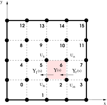
Fig. 4: The horizontal direction flows of area considered for the square $s$ (colored by gray) in the equidensity constraint (4).

In fact, the second summand in (8) can be replaced by

$$\sum_{s\in\mathcal{S}(\mathcal{G})}(\lambda_{s}+Z)(\mathfrak{eqd}(s)-b_{s})$$

for any $Z$ without changing the minimization of $\mathfrak{L}$ since

$$Z\sum_{s\in\mathcal{S}(\mathcal{G})}(\mathfrak{eqd}(s)-b_{s})=0~{}.$$

Thus, important are not the values of $\lambda_{s}$ but only their differences, and the singularity can be treated by an additional constraint, say, $\sum_{s}d_{s}\lambda_{s}=0$, where $d_{s}=1~{}\forall s\in\mathcal{S}(\mathcal{G})$ (the introduction of $d_{s}$ is necessary for the recursion of the multilevel solver; see Section 3.2.1). The additional term in $\mathfrak{L}({\bf u},\lambda)$ is $\eta\sum_{s}d_{s}\lambda_{s}$, where $\eta$ is a “pseudo-Lagrange” multiplier. The following proposition (with $k=1$) motivates the non-singularity of $\mathfrak{L}$ with $\sum_{s}d_{s}\lambda_{s}=0$.

Proposition 1.

Given a symmetric $n\times n$ matrix $A$, for which $rank(A)=n-k$, let $x_{i},~{}i=1,...,k$ be an orthgonal basis of the null space of $A$, that is, $Ax_{i}=0$. Then the following block matrix $B$ is nonsingular

$$B=\left(\begin{array}[]{c|c}A&X\\ \hline\cr X^{T}&0\end{array}\right),$$

where $X=(x_{1},...,x_{k})$ is an $n\times k$ matrix of rank $k$.

Proof.

Let $y$ be any vector in $\mathbb{R}^{n+k}$. Denote by $y^{\prime}$ the first $n$ components of $y$ and by $y^{\prime\prime}$ the last $k$ components, that is, $y=\left({y^{\prime}}\over{y^{\prime\prime}}\right)$. We will prove that if $By=0$, then $y=0$. The vector $By$ can be written in the following block form:

$$By=\left(\begin{array}[]{c}Ay^{\prime}+Xy^{\prime\prime}\\ \hline\cr X^{T}y^{\prime}\end{array}\right).$$

Multiplying $Ay^{\prime}+Xy^{\prime\prime}=0$ by $X^{T}$ from the left implies that $y^{\prime\prime}=0$, and hence $Ay^{\prime}=0$ and $y^{\prime}=\sum_{i=1}^{k}\alpha_{i}x_{i}$. Substituting the last relation into each of the last $k$ rows of $B$ implies $x_{j}^{T}y^{\prime}=x_{j}^{T}\sum_{i=1}^{k}\alpha_{i}x_{i}=\alpha_{j}x_{j}^{T}x_{j}=0$ and thus $\alpha_{j}=0$ for $j=1,...,k$ yielding $y^{\prime}=0$. Since $y^{\prime}=0$ and $y^{\prime\prime}=0$ we may conclude that $y=0$ as needed. ∎

The second kind of singularity in (9) may appear from possible empty squares. This can be treated by adding a summand to (8) that minimizes the total sum of all corrections $\beta\sum_{i}{\bf u}_{i}^{2}$, that is, adds a $2\beta$-term to the diagonal of $\nabla_{{\bf u}}\mathfrak{L}$, where $\beta$ is small enough to cause only negligible change in a solution. This will prevent the inclusion of zero-rows in $\nabla_{{\bf u}}\mathfrak{L}$, while possibly also bounding the size of each correction in the solver below.

To summarize, the pseudo-Lagrangian functional $\mathfrak{L}$ for our correction problem with equality constraint is

$$\mathfrak{L}({\bf u},\lambda,\eta)=\frac{1}{2}\sum_{i,j}q_{ij}{\bf u}_{i}{\bf u}_{j}+\sum_{i}l_{i}{\bf u}_{i}+\beta\sum_{i}{\bf u}_{i}^{2}+\sum_{s\in\mathcal{S}(\mathcal{G})}\lambda_{s}(\sum_{i}a_{si}{\bf u}_{i}-b_{s})+~{}\eta\sum_{s\in\mathcal{S}(\mathcal{G})}d_{s}\lambda_{s}~{},$$ (10)

leading to the following system of equations

$$\begin{array}[]{ll}\frac{1}{2}\sum_{j}q_{ij}{\bf u}_{j}+l_{i}+2\beta{\bf u}_{i}+\sum_{s\in\mathcal{S}(\mathcal{G})}\lambda_{s}a_{si}=0~{},{}&\forall i~{}\text{s.t.}~{}{\bf u}_{i}\in{\bf u}\setminus\mathcal{B}_{u}(\mathcal{G})\setminus\mathcal{B}_{v}(\mathcal{G})\\ \sum_{i}(a_{si}{\bf u}_{i}-b_{s})+~{}\eta d_{s}=0~{},{}&\forall s\in\mathcal{S}(\mathcal{G}){}\\ \sum_{s\in\mathcal{S}(\mathcal{G})}d_{s}\lambda_{s}=0~{}.&\end{array}$$ (11)

Since in real world situations the total area is usually bigger than the total area of all the vertices, the redefined minimization problem under inequality constraints will generally have the form

$$\begin{array}[]{ll}\mbox{{minimize}}&\mathfrak{E}({\bf u})~{}~{}~{}~{}~{}~{}~{}~{}~{}~{}~{}~{}~{}~{}~{}~{}~{}~{}~{}~{}~{}~{}~{}~{}~{}~{}~{}~{}(\text{given by }(\ref{E-with-q-and-l}))\\ \mbox{{subject to}}&\mathfrak{eqd}(s)\leq b_{s}~{},~{}\forall s\in\mathcal{S}(\mathcal{G})~{}~{}~{}(\text{given by }(\ref{eqd-with-a-and-b}))~{}.\end{array}$$ (12)

3.2 Multilevel solver for problem (12)

To solve the constrained minimization problem (12), we use multigrid techniques: standard geometric coarsening, linear interpolation, Correction Scheme for the energy minimization and the Full Approximation Scheme for the equidensity inequality constraints; all are presented in Section 3.2.1. In addition, we have developed a fast window minimization relaxation as explained in Section 3.2.2. The multilevel cycle is schematically summarized in Section 3.2.3 in Algorithm 2D-layout-correction.

3.2.1 Coarsening scheme

When the geometry of the problem is known we can choose a coarser grid by the usual elimination of every other line, as shown in Figure 5. The correction computed at the coarse grid points will be interpolated and added to the fine grid current approximation. Let us introduce the notation distinguishing between fine and coarse level variables and functions. By lowercase and uppercase letters we will refer to the variables, indexes, and coefficients of the fine (${\bf u}_{i}$, $i$, $q_{j}$, etc.) and the coarse (${\bf U}_{I}$, $I$, $Q_{J}$, etc.) levels, respectively. The subscripts $f$ and $c$ will be used to describe the energy $\mathfrak{E}_{f}$ and $\mathfrak{E}_{c}$ and pseudo-Lagrangian $\mathfrak{L}_{f}$ and $\mathfrak{L}_{c}$ functions at the fine and the coarse levels, respectively.

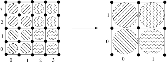
Fig. 5: Geometric coarsening. The equidensity constraints of every four similarly patterned squares at the fine level form one equidensity constraint at the coarse level.

Thus, the minimization part of the pseudo-Lagrangian (10) at the fine level is

$$\mathfrak{E}_{f}=\frac{1}{2}\sum_{ij}q_{ij}{\bf u}_{i}{\bf u}_{j}+\sum_{i}l_{i}{\bf u}_{i}~{}~{}~{}.$$ (13)

(Note that we have omitted the $\beta$ term from the following derivation since it is merely an artificial added term.) Given a current approximation $\tilde{{\bf u}}$ of the fine level solution ${\bf u}$ and a correction function ${\bf U}$ calculated at the coarse level variables ${\bf U}$, $\tilde{{\bf u}}$ will be corrected by

$$\tilde{{\bf u}}_{i}\leftarrow\tilde{{\bf u}}_{i}+\sum_{I\ni i}\alpha_{iI}{\bf U}_{I}~{},$$ (14)

where the notation $\sum_{I\ni i}$ means that the sum is running over all coarse gridpoints $p_{I}$ from which standard bilinear interpolation is made to the fine gridpoint $p_{i}$.

Expressing the fine level energy functional $E_{f}$ in terms of the coarse variables by substituting (14) into (13) yields

$$\mathfrak{E}_{f} =\frac{1}{2}\sum_{ij}q_{ij}(\tilde{{\bf u}}_{i}+\sum_{I\ni i}\alpha_{iI}{\bf U}_{I})(\tilde{{\bf u}}_{j}+\sum_{J\ni j}\alpha_{jJ}{\bf U}_{J})+\sum_{i}l_{i}(\tilde{{\bf u}}_{i}+\sum_{I\ni i}\alpha_{iI}{\bf U}_{I})=$$

$$=\frac{1}{2}\sum_{IJ}Q_{IJ}{\bf U}_{I}{\bf U}_{J}+\sum_{I}L_{I}{\bf U}_{I}+C~{},$$

where ${Q}_{IJ}=\sum_{\begin{subarray}{c}i\in I\\ j\in J\end{subarray}}{q}_{ij}\alpha_{iI}\alpha_{jJ}$, $L_{I}=\sum_{\begin{subarray}{c}j\\ i\in I\end{subarray}}{q}_{ij}\tilde{{\bf u}}_{j}\alpha_{iI}+\sum_{i\in I}l_{i}\alpha_{iI}~{}$ and $C$ is a constant. Thus, the coarse level energy functional will be of the same structure as the fine level one, namely,

$$\mathfrak{E}_{c}=\frac{1}{2}\sum_{IJ}Q_{IJ}{\bf U}_{I}{\bf U}_{J}+\sum_{I}L_{I}{\bf U}_{I}~{}.$$

For each fine square $s$ the equidensity constraint $\mathfrak{eqd}(s)$ is given by (7). The coarse equidensity constraints are constructed by merging $2\times 2$ fine squares into one coarse square $S$. The expression ”$s\in S$” will refer to running over the four fine squares $s$ that form the coarse square $S$ (see Figure 5). The $S$-th planar equidensity constraint of the coarse level (in the case of equality constraints only) is obtained again by the substitution of (14):

$$\sum_{s\in S}\sum_{i}a_{si}{\bf u}_{i}-\sum_{s\in S}b_{s} = \sum_{I}A_{SI}{\bf U}_{I}-B_{S}~{},$$

where $A_{SI}=\sum_{i\in I}\sum_{s\in S}a_{si}\alpha_{iI}$ and $B_{S}=\sum_{s\in S}(b_{s}-\sum_{i}a_{si}\tilde{{\bf u}}_{i})$. Similarly (in the case of equality constraints), the additional $\eta$-constraint over all squares at the coarse level as inherited from the fine level is $\sum_{S}D_{S}\Lambda_{S}=0$, where $D_{S}=\sum_{s\in S}d_{s}$.

To complete the description of the coarse equations, we still need to transfer the equidensity inequality constraints. For this purpose we will use the Full Approximation Scheme (FAS), which is the general multigrid strategy applied to nonlinear problems (see [3, 4, 14]). In fact, there is no need for the FAS for the equality equidensity constraints since it is a linear problem that can be solved by the regular Correction Scheme (CS). The FAS-like coarsening rules are needed and applied only on the set of equations derived from the equidensity inequalities. Thus, our scheme is a combination of the correction scheme for the energy equations derived from (13) and (14) and FAS-like rules for the equidensity equations.

To derive these equations we need to calculate the residuals for both the fine and coarse grids. If $\mathfrak{L}_{f}$ is the pseudo-Lagrangian of the fine level system defined by

$$\mathfrak{L}_{f}=\mathfrak{E}_{f}+\sum_{s}\lambda_{s}(\sum_{i}a_{si}{\bf u}_{i}-b_{s})+\eta\sum_{s}d_{s}\lambda_{s}~{}~{}~{},$$ (15)

where $\mathfrak{E}_{f}$ is given by (13), then the ${\bf u}_{i}$-th residual of $\nabla\mathfrak{L}_{f}$, where $\tilde{\lambda}_{s}$ is the current value of the Lagrange multiplier ${\lambda}_{s}$, is

$$r_{i}^{\mathfrak{E}}=-l_{i}-\frac{1}{2}\sum_{j}q_{ij}\tilde{{\bf u}}_{j}-\sum_{s}\tilde{\lambda}_{s}a_{si}.$$

Thus, the residual corresponding to the variable ${\bf U}_{I}$ of $\nabla\mathfrak{L}_{c}$ (where $\nabla\mathfrak{L}_{c}$ is the coarse level system of equations analogous to (15)) is

$$R_{I}^{\mathfrak{E}}=\sum_{i\in I}\alpha_{iI}r_{i}^{\mathfrak{E}}~{},$$ (16)

where $\alpha_{iI}$ are as in (14); that is, the fine-to-coarse transfer is the adjoint of our coarse-to-fine interpolation. The residual of the $s$-th equidensity constraint is

$$r_{s}^{\mathfrak{eqd}}=b_{s}-\sum_{i}a_{si}\tilde{{\bf u}}_{i}-\tilde{\eta}d_{s}~{},$$

where $s$ runs over all fine squares and $\tilde{\eta}$ is the current value of ${\eta}$. Therefore, the coarse equidensity residual of square $S$ is

$$R_{S}^{\mathfrak{eqd}}=\sum_{s\in S}r_{s}^{\mathfrak{eqd}}~{}.$$ (17)

Finally the residual of the $\eta$-constraint is

$$r_{\eta}=-\sum_{s}d_{s}\tilde{\lambda}_{s}=R_{H}.$$

Denote by $LP(I)$ the linear part of the ${\bf U}_{I}$-th equation in the system $\nabla\mathfrak{L}_{c}$

$$LP(I)=\frac{1}{2}\sum_{J}Q_{IJ}{\bf U}_{J}+\sum_{S}\Lambda_{S}A_{SI}.$$

From the FAS rule for the $I$-th coarse equation stating that $LP(I)=R_{I}^{\mathfrak{E}}+$ the current approximation of $LP(I)~{}$, we can derive the $I$-th $\nabla\mathfrak{L}_{c}$ equation

$$\frac{1}{2}\sum_{J}Q_{IJ}{\bf U}_{J}+\sum_{S}\Lambda_{S}A_{SI}-R_{I}^{\mathfrak{E}}-\frac{1}{2}\sum_{J}Q_{IJ}{\bf U}_{J}^{0}-\sum_{S}\Lambda_{S}^{0}A_{SI}=0,$$ (18)

where $R_{I}^{\mathfrak{E}}$ is given by (16), ${\bf U}_{J}^{0}=0$ and $\Lambda_{S}^{0}=\frac{1}{4}\sum_{s\in S}\tilde{\lambda}_{s}$. Similarly, the $S$-th square coarse equation for the equality (inequality) constraint is

$$\sum_{I}A_{SI}{\bf U}_{I}+HD_{S}-R_{S}^{\mathfrak{eqd}}-\sum_{I}A_{SI}{\bf U}_{I}^{0}-H^{0}D_{S}=(\leq)0~{},$$ (19)

where $R_{S}^{\mathfrak{eqd}}$ is given by (17). The last equation for the $H$-constraint is

$$\sum_{S}D_{S}\Lambda_{S}-R_{H}-\sum_{S}D_{S}\Lambda_{S}^{0}=0.$$ (20)

Note that equations (18) to (20) are the coarse grid equations analog to the system (11). (A $2\beta{\bf U}_{I}$ term may be added to (18) for stability if needed.) The correction received from the coarse level for the ${\bf u}$ variables is given by (14) and for the Lagrange multipliers $\lambda$ by

$$\tilde{\lambda}_{s}\leftarrow\tilde{\lambda}_{s}+\Lambda_{\begin{subarray}{c}S\ni s\end{subarray}}-\Lambda_{\begin{subarray}{c}S\ni s\end{subarray}}^{0}~{}.$$ (21)

3.2.2 Relaxation

In our multigrid solver, as usual, the relaxation process is employed as the smoother of the error of the approximation, before the construction of the coarse level system and immediately after interpolation from the coarse level. For this purpose we have developed the Window relaxation procedure, which extracts from the entire system small subproblems of $m\times m$ squares and solves each separately, as explained below. The running time of the entire relaxation process strongly depends on the algorithm for solving one window. There exist many versions of well-known algorithms for the quadratic minimization problem under linear inequality constraints (for a survey see [1]). However, since each window need be solved only to a first approximation (because of the iterative nature of the overall algorithm), in order to keep the running time low, we have implemented a simple algorithm for approximately solving each single window, as presented in SingleWindowSolver.

Let $\mathcal{W}=\{s\in\mathcal{S}(\mathcal{G})|\text{ all squares within an $m\times m$ super-square}\}$ be a window of squares. To solve the quadratic minimization problem in $\mathcal{W}$, we fix at their current position all ${\bf u}$ outside $\mathcal{W}$, as well as all those that are on the boundary of $\mathcal{W}$ and represent movement perpendicular to the boundary. The minimization is done under the set of equidensity constraints for the squares $s\in\mathcal{W}$. The solution process for each single window is a simplified version of the active set method and is iterative. At each iteration $t$, for a given $\tilde{{\bf u}}$ we first extract the set (denoted by $S_{t}$) of squares for which the respective inequality equidensity constraints are violated or almost violated:

$$S_{t}=\{s\in\mathcal{W}~{}|~{}\mathfrak{eqd}(s)>b_{s}-\epsilon\}~{},$$

where $\epsilon$ is positive and sufficiently small but not too small to make $S_{t}$ numerically unstable (we have used $\epsilon=0.0001*$(the square’s area)). Then the inequality constraints of $S_{t}$ are set to equalities ignoring the other inequality constraints. Let $\mathbb{\mathcal{P}}_{\mathcal{W}}$ be the set of all displacement indexes inside $\mathcal{W}$ (including those on the boundary of $\mathcal{W}$ directing parallel to it). For every ${\bf u}_{i},i\in\mathbb{\mathcal{P}}_{\mathcal{W}}$ we associate a correction variable $\delta_{i}$ and we reformulate the pseudo-Lagrangian for $\mathcal{W}$ as a functional of the $\delta_{i}$ variables as follows:

$$\mathfrak{L}_{\mathcal{W}}(\delta,\lambda)=\frac{1}{2}\sum_{i,j\in\mathbb{\mathcal{P}}_{\mathcal{W}}}q_{ij}(\tilde{{\bf u}}_{i}+\delta_{i})(\tilde{{\bf u}}_{j}+\delta_{j})+\frac{1}{2}\sum_{\begin{subarray}{c}i\in\mathbb{\mathcal{P}}_{\mathcal{W}},~{}j\not\in\mathbb{\mathcal{P}}_{\mathcal{W}}\end{subarray}}q_{ij}(\tilde{{\bf u}}_{i}+\delta_{i})\tilde{{\bf u}}_{j}+\\ \sum_{i\in\mathbb{\mathcal{P}}_{\mathcal{W}}}l_{i}(\tilde{{\bf u}}_{i}+\delta_{i})+\beta\sum_{i\in\mathbb{\mathcal{P}}_{\mathcal{W}}}(\tilde{{\bf u}}_{i}+\delta_{i})^{2}+\sum_{s\in S_{t}}\lambda_{s}(\sum_{i\in\mathbb{\mathcal{P}}_{\mathcal{W}}}a_{si}\tilde{{\bf u}}_{i}-b_{s})~{},$$ (22)

where $\tilde{{\bf u}}_{i}$ is the current value of ${\bf u}_{i}$ and the $\beta$ term is added for stability with $\beta=1$. Solving $\nabla\mathfrak{L}_{\mathcal{W}}(\delta,\lambda)=0$ we obtain the corrections $\delta_{i}$ for $\tilde{{\bf u}}_{i},i\in\mathbb{\mathcal{P}}_{\mathcal{W}}$, which confine the respective active set variables to the boundary of the equality constraints manifold. However, while accepting this correction we may violate other inequality constraints that were already satisfied at the previous iteration $t-1$. Let us call this set of new unsatisfied constraints $\overline{S}_{t}$. One way to overcome this problem is to accept only a partial correction $\theta\delta_{i}$, $i\in\mathbb{\mathcal{P}}_{\mathcal{W}}$, where $\theta$ is the smallest number that brings some constraint from $\overline{S}_{t}$ to equality. Accepting the correction $\theta\delta_{i}$ does not violate any constraint from $\overline{S}_{t}$. At this point we accept this partial correction and continue to the next iteration $t+1$, excluding from the redefined $S_{t}$ the set of satisfied (by equality) constraints from $S_{t}$ with negative Lagrange multipliers $\lambda_{s}$.

SingleWindowSolver($\mathcal{W}$, $\tilde{{\bf u}}$)
begin
	$t=0$
	Repeat until ”optimal enough” (explained at the end of Section 4)
		If $t=0$
			$S_{t}=\{$the violated equidensity constraints$\}$
		Else
			$S_{t}=\{$the violated equidensity constraints$\}\setminus$
$\{$those from iteration $t-1$ which satisfy equality and have $\lambda_{s}<0\}$
		Solve $\nabla\mathfrak{L}_{\mathcal{W}}(\delta,\lambda)=0$ and extract the smallest $\theta$
		Accept the correction $\tilde{{\bf u}}\leftarrow\tilde{{\bf u}}+\theta\delta$
		$t\leftarrow t+1$
end

To achieve corrections for all variables, we will cover by these windows the entire area in red-black order [14]. For computational reasons we have chosen to apply this relaxation for very small windows (of size $4\times 4$ squares). To minimize the effects of the boundary constraints in the windows and to enforce the equidensity constraints over different super-squares, we scan the entire domain two more times: once with half-window size shift in the horizontal direction and once in the vertical. Thus the overall relaxation process covers the domain three times.

3.2.3 The multilevel cycle

Having defined the window relaxation, the interpolation, and the coarsening scheme, the multilevel cycle naturally follows. Starting from the given approximation $(\tilde{x},\tilde{y})$, discretize the domain by a standard grid on which the ${\bf u}$ variables are initially defined. Construct the system of equations (11), and solve for the ${\bf u}$ variables as follows. After applying $\nu_{1}$ window relaxation sweeps, define the coarser level equations for the coarser grid, apply $\nu_{1}$ window relaxation sweeps there, and continue to a still coarser level. This process is recursively repeated until a small enough problem is obtained. Solve this coarsest problem directly, and start the uncoarsening stage by interpolating the solution of the coarse level to the finer levels followed by $\nu_{2}$ window relaxation sweeps on the finer level. Repeat until the correction to the original problem is obtained. This entire multilevel cycle, usually referred to as the V-cycle, is summarized in procedure V-cycle-correction below, where the superscript index refers to the level number. (We have used $\nu_{1}=\nu_{2}=3$).

V-cycle-correction($\mathcal{G}^{i}$, ${\bf u}^{i}$, $\mathcal{C}^{i}$, $\lambda^{i}$, $\nabla\mathfrak{L}^{i}$)
begin
	If $\mathcal{G}^{i}$ is a small enough grid
		Solve the problem exactly
	Else
		Set ${\bf u}^{i}=0$
		Apply $\nu_{1}$ Window relaxation sweeps
		Construct $\mathcal{G}^{i+1}$ the coarse level grid
		Define $\mathcal{C}^{i+1}$ to be the set of equidensity constraints
		Initialize the system of equations $\nabla\mathfrak{L}^{i+1}$ given by (18)-(20)
		Initialize ${\bf u}^{i+1}$ and $\lambda^{i+1}$
		V-cycle-correction($\mathcal{G}^{i+1}$, ${\bf u}^{i+1}$, $\mathcal{C}^{i+1}$, $\lambda^{i+1}$, $\nabla\mathfrak{L}^{i+1})$
		Interpolate from level $i+1$ to level $i$ using (14) and (21)
		Apply $\nu_{2}$ Windows relaxation sweeps
Return ${\bf u}^{i}$

3.3 The Full MultiGrid external driving routine

The solution of (11) is primarily dependent on the chosen grid size. To enforce equidensity at all scales, it can be used within the Full MultiGrid (FMG) framework. This is done by using a sequence of increasing grid sizes (progressively finer meshsizes), while employing a small number of V-cycles for each grid size. We emphasize that the original problem (2) is highly nonlinear, while the system of equations with corrections in term of the displacement ${\bf u}$ is linearized around the current solution $(\tilde{x},\tilde{y})$. Therefore, only a small correction should actually be taken from the ${\bf u}$ displacements when these $(\tilde{x},\tilde{y})$ are being updated. Then, a new linear system can be formulated around the new solution to obtain a new correction, and so forth. Thus, by small steps of corrections we solve the original nonlinear problem via the corrections calculated from the linear system of equidensity constraints. For instance, we have tried to employ grids of sizes: 2, 4, 8, … up to a grid with number of squares comparable to the number of nodes in the graph. For each grid size the corresponding set of equations (in terms of the displacement ${\bf u}$) is solved either directly (for small enough grids) or by employing the V-cycles described in Section 3.2.3. In either cases the obtained solution ${\bf u}$ is interpolated back to the $(x,y)$ variables, introducing the desired correction to the original variables of the problem. Various driving routines can be actually used: each chosen grid size may be solved more than once (e.g., use grids 2, 2, 4, 4, 8,…); the entire sequence of grids may be repeated (e.g., 2, 2, 4, 4, 8,… , 2, 2, 4, 4, 8,…), and so on. (see Section 4 for examples). These parameters should in fact be optimized for each application according to the concrete needs of the model.

The entire algorithm for the two-dimensional layout correction is summarized below in Algorithm 2D-layout-correction, where the superscript 0 refers to the current chosen grid size.

2D-layout-correction(graph $G$, current layout $(\tilde{x},\tilde{y})$)
begin
	Apply for a sequence of grid sizes
		Construct and initialize $\mathcal{G}^{0}$, ${\bf u}^{0}$
		Define $\mathcal{C}^{0}$ to be the set of equidensity constraints
		Initialize the system of equations $\nabla\mathfrak{L}^{0}$
		V-cycle-correction($\mathcal{G}^{0}$, ${\bf u}^{0}$, $\mathcal{C}^{0}$, $\lambda^{0}$, $\nabla\mathfrak{L}^{0}$)
		Update $(\tilde{x},\tilde{y})$ from ${\bf u}^{0}$
Return $(\tilde{x},\tilde{y})$

4 Examples of graph drawing layout correction

As previously mentioned, the graph drawing problem is of interest for many applications. Therefore, we have chosen to demonstrate the abilities of our algorithm for this problem. In this section we will present several results of the two-dimensional layout correction algorithm using inequality constraints. The set of examples is shown in Figures 6 and 10 to 13, each organized in two columns. The initial and final layouts of the graph are shown in the same row, in the left and the right columns, respectively. Note that finalizing the ”nice graph” representation of these examples is beyond the scope of this work. The various ”beautifying” procedures used by different applications may, of course, be used at the end of our cycles to enhance the visualization results.

The first example consists of a mesh graph with three holes (Figure 6, row (a)). It is intended to demonstrate that the empty space stays empty and the energy is thus kept low. More complicated examples are shown in Figure 6, rows (b) and (c). The initial optimal positions of the mesh’s vertices were randomly changed by independent shifts in different directions within a distance $d$:

$$d~{}\leq~{}\left\{\begin{array}[]{ll}2h_{x}&\text{ in example (b)}\\ 4h_{x}&\text{ in example (c)}~{},\\ \end{array}\right.$$

where $h_{x}$ is the length of a square on the initially taken 32x32 grid, such that the mesh size of the graph is actually $2h_{x}$. Let us call these meshes $M_{1}$ and $M_{2}$, respectively. While the correction of $M_{1}$ looks really nice, two switched vertices at the right-hand side of $M_{2}$ demonstrate a weak point in our algorithm that certainly must be improved by a local ”beautifying” procedure, which in general depends on the real application. The initial layout (c1) is more complicated than (b1), while the desired final layouts are similar.

A typical example of the energy behavior is presented in Figures 7-9. These figures refer to the mesh example in Figure 6-(c). The general energy minimization progress is shown in Figure 7. In this example the driving routine alternates between two grid size V-cycles: each odd V-cycle solves the correction problem for the 16x16 grid, while even V-cycles improve the previous iterations with the grid 32x32. Figures 8 and 9 show the energy behavior of the Window relaxations (without V-cycles) for 16x16 grid iterations and alternately 16x16 and 32x32 grid sizes, respectively. Clearly, the V-cycle algorithm is more powerful in minimizing the energy than just employing the Window relaxations.

A more complicated example is shown in Figure 10 in which the 64x64 mesh graph randomly perturbed by vertex shifts (up to $2h_{x}$ of a 64x64 grid), compressed at the left bottom corner and augmented by 50 randomly chosen edges (Figure 10-(a)). The final result of the algorithm is presented in Figure 10-(b), where all vertices are placed almost at their optimal locations (note the different scales of the two figures). We have used 2-FMG cycles with 2 V-cycles at each level as the main driving routine. Such a driving routine works with the following grid sizes: 2, 2, 4, 4, 8, 8, …, 128, 128, 2, 2, 4, 4, and so forth. After these 2-FMG cycles the total energy was very close to its real minimum and additional iterations have only slightly corrected the layout. The next experiment consists of the 64x64 compressed mesh with three holes. The initial and final layouts are presented in Figures 11-(a) and 11-(b), respectively.

Two additional examples demonstrate the layout corrections for graphs whose vertices have nonequal volumes (see Figures 12 and 13). In both cases the initial layout of these graphs was random.

In spite of the promising results presented above, the algorithm has not yet been optimized. However, it is already clear that several parameters must for efficiency be kept very small. For example: (1) the number of Window relaxation iterations should be fixed between 1 and 3; (2) ”optimal enough” in SingleWindowSolver means less than 6 iterations and (3) the size of $\mathcal{W}$ in SingleWindowSolver is very robust, that is, the same results can be obtained with sizes $4$x$4$, $8$x$8$, and $16$x$16$. We have used only $4$x$4$ as it runs the fastest.

$\begin{array}[]{cc}\includegraphics[width=144.54pt]{m32hole_start.pdf}&\includegraphics[width=144.54pt]{m32hole_98_10.pdf}\\[2.84544pt] \mbox{\bf(a1)}&\mbox{\bf(a2)}\\ \includegraphics[width=144.54pt]{rnd_mesh_16_start_2.pdf}&\includegraphics[width=144.54pt]{rnd_mesh_16_05_2.pdf}\\[2.84544pt] \mbox{\bf(b1)}&\mbox{\bf(b2)}\\ \includegraphics[width=144.54pt]{rnd2_mesh_16_start.pdf}&\includegraphics[width=144.54pt]{rnd2_mesh_16_05.pdf}\\[2.84544pt] \mbox{\bf(c1)}&\mbox{\bf(c2)}\end{array}$

Fig. 6: Examples of the 2D-layout of graphs with equal vertices.

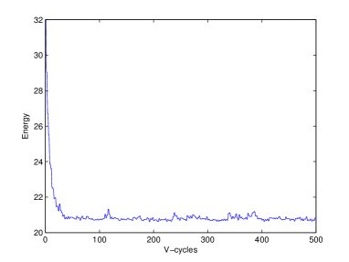
Fig. 7: Energy behavior of the mesh at Figure 6-(c), when employing complete V-cycles with $16\times 16$ and $32\times 32$ alternately.

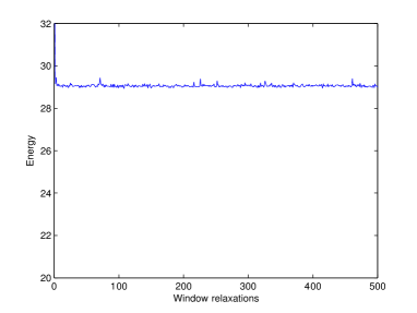
Fig. 8: Energy behavior of Window relaxation iterations ($16\times 16$ grid) of the mesh at Figure 6-(c).

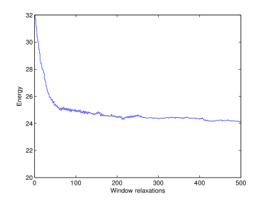
Fig. 9: Energy behavior of Window relaxation iterations ($16\times 16$ and $32\times 32$ grids) of the mesh at Figure 6-(c).

$\begin{array}[]{cc}\includegraphics[width=180.67499pt]{r64a_start_en.pdf}&\includegraphics[width=180.67499pt]{r64a_finsh.pdf}\\ \textbf{(a)}&\textbf{(b)}\end{array}$

Fig. 10: Example of the layout of the $64\times 64$ mesh with additional random edges (note the different scales of the two figures): (a) starting from a compressed and perturbed configuration at the bottom-left corner, (b) the resulting picture using V-cycles.

$\begin{array}[]{cc}\includegraphics[width=180.67499pt]{rhm64b.pdf}&\includegraphics[width=180.67499pt]{rhm64.pdf}\\ \textbf{(a)}&\textbf{(b)}\end{array}$

Fig. 11: Example of the $64\times 64$ mesh with three holes layout (note the different scales of the two figures): (a) starting from a compressed and perturbed configuration at the bottom-left corner, (b) the resulting picture using V-cycles.

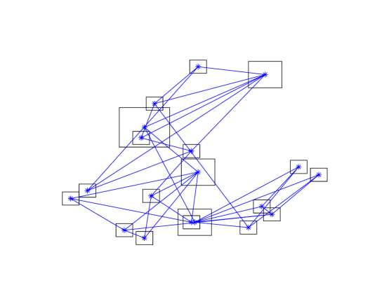
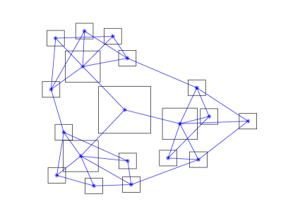
Fig. 12: Example of the 2D-layout of a graph with nonequal volumes.

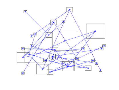
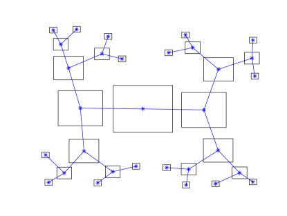
Fig. 13: An example of the 2D-layout of a 5-level binary tree with non-equal vertices.

5 Conclusions

We have presented a linear time multilevel algorithm for solving correction to the nonlinear minimization problem under planar (in)equality constraints. By introducing a sequence of grids over the domain and a new set of global displacement variables defined at those grid points, we formulated the minimization problem under planar equidensity constraints and solved the resulting system of equations by multigrid techniques. This approach enabled fast collective corrections for the optimization objective components. We believe that this formulation can open a new direction for the development of fast algorithms for efficient space utilization goals. Among many possible motivating applications [2, 7, 9, 8, 6, 12, 5, 11, 13] we focused on the demonstration of the method on the graph visualization problem with efficient space utilization demand.

We recommend this multilevel method as a general practical tool in solving, possibly together with other tools, the nonlinear optimization problem under planar (in)equality constraints.

6 Acknowledgments

This work was supported in part by the Office of Advanced Scientific Computing Research, Office of Science, U.S. Department of Energy, under Contract DE-AC02-06CH11357.

The submitted manuscript has been created in part by UChicago Argonne, LLC, Operator of Argonne National Laboratory (”Argonne”). Argonne, a U.S. Department of Energy Office of Science laboratory, is operated under Contract No. DE-AC02-06CH11357. The U.S. Government retains for itself, and others acting on its behalf, a paid-up nonexclusive, irrevocable worldwide license in said article to reproduce, prepare derivative works, distribute copies to the public, and perform publicly and display publicly, by or on behalf of the Government.

References

- [1] M. Avriel. Nonlinear Programming: Analysis and Methods. Dover Publications, 2003.
- [2] G. Di Battista, P. Eades, R. Tamassia, and I. Tollis. Graph Drawing: Algorithms for the Visualization of Graphs. Prentice Hall PTR, Upper Saddle River, NJ, USA, 1998.
- [3] A. Brandt. Multi-level adaptive solutions to boundary-value problems. Math. Comp., 31(138):333–390, April 1977.
- [4] A. Brandt and D. Ron. Chapter 1 : Multigrid solvers and multilevel optimization strategies. In J. Cong and J. R. Shinnerl, editors, Multilevel Optimization and VLSICAD, pages 1–69. Kluwer, 2003.
- [5] M. Cardei and J. Wu. Energy-efficient coverage problems in wireless ad hoc sensor networks.
- [6] Zvi Drezner. Facility Location: A Survey of Applications and Methods. Springer, New York, 1995.
- [7] P. A. Eades. A heuristic for graph drawing. In Congressus Numerantium, volume 42, pages 149–160, 1984.
- [8] D. Harel and A. Inger. On the aesthetic layout of higraphs. submitted, 2006.
- [9] David Harel. On visual formalisms. Commun. ACM, 31(5):514–530, 1988.
- [10] Joe Marks, editor. Graph Drawing, 8th International Symposium, GD 2000, Colonial Williamsburg, VA, USA, September 20-23, 2000, Proceedings, volume 1984 of Lecture Notes in Computer Science. Springer, 2001.
- [11] S. Meguerdichian, F. Koushanfar, M. Potkonjak, and M. B. Srivastava. Coverage problems in wireless ad-hoc sensor networks. volume 3, pages 1380–1387, 2001.
- [12] Seapahn Meguerdichian, Farinaz Koushanfar, Miodrag Potkonjak, and Mani B. Srivastava. Coverage problems in wireless ad-hoc sensor networks. In INFOCOM, pages 1380–1387, 2001.
- [13] G.-J. Nam and J. Cong. Modern Circuit Placement. Springer, New York, 2007.
- [14] U. Trottenberg, C.W. Oosterlee, and A. Schuller. Multigrid. Academic Press, Orlando, FL, 2001.