Random numbers from the tails of probability distributions using the transformation method

Abstract

The speed of many one-line transformation methods for the production of, for example, Lévy alpha-stable random numbers, which generalize Gaussian ones, and Mittag-Leffler random numbers, which generalize exponential ones, is very high and satisfactory for most purposes. However, for the class of decreasing probability densities fast rejection implementations like the Ziggurat by Marsaglia and Tsang promise a significant speed-up if it is possible to complement them with a method that samples the tails of the infinite support. This requires the fast generation of random numbers greater or smaller than a certain value. We present a method to achieve this, and also to generate random numbers within any arbitrary interval. We demonstrate the method showing the properties of the transform maps of the above mentioned distributions as examples of stable and geometric stable random numbers used for the stochastic solution of the space-time fractional diffusion equation.

1 Introduction

Many numerical methods for the generation of random numbers represent the main body of the probability density using a fast method and the tails using an alternative method. A famous example is the Ziggurat method by Marsaglia and Tsang [27]. Fig. 1 depicts the situation schematically. A reason for this apparent complication is that the method for the main body works best and fastest on a finite support or is specially designed for the main body in terms of accuracy or speed. Handling the tails efficiently is often more involved, especially with difficult non-invertible densities with infinite support. Since rarely needed, variates from the tail can safely be generated by a slower method [4, 27, 28]. Overall, a significant speed-up can be achieved. In this paper we show how to sample directly and efficiently via a rejection technique a random number $X$ such that $X>x$ or $X<x$ where $x\in(-\infty,+\infty)$ at least within the limits of the numerical representation. This is achieved by using properties of the transform representation of the distributions. The examples we use for demonstration are the Lévy $\alpha$-stable  [21, 31, 32] and the Mittag-Leffler one-parameter probability densities [15]. A transformation formula for the former is well known [2, 42], while the transform representation of the latter was discovered [5, 16, 17, 18, 19, 20, 33] and applied [9, 8, 10] only recently. The two distributions are generalizations of the Gaussian and exponential distribution respectively and play an important role together for the solution of the space-time fractional diffusion equation.

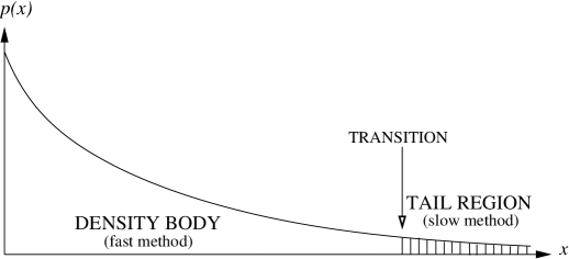
Figure 1: Schematic illustration of using two methods for sampling a distribution. A fast method may be available only for the body, while the tails can be sampled with a slower method.

Our rejection concept is general for any distribution that provides a transform representation. It can sample efficiently from arbitrary infinite or finite intervals as opposed to other existing methods that are designed especially for certain densities. In this work we do not consider the technical details of a speed-optimized implementation, but explain the basis of the algorithm and show example applications. The method is based on properties of the two-dimensional transform maps that seem unnoticed yet.

The assumption for using the method introduced here is that the tail region requires high accuracy due to high demands on statistics as well as speed. The transformation formula by Chambers, Mallows and Stuck [2] for example is exact and for most applications the recommended method for the production of Lévy $\alpha$-stable random numbers [42]. The replacement of the tails by a simple invertible Pareto function is not totally appropriate because this is only an asymptotic approximation; moreover it introduces a transition region. The more sophisticated and smooth this transition, the more complicated and slower the overall procedure. Such a replacement of the tail contrasts the initial goal of speed. But the most demanding contemporary applications of random numbers [29, 42], as of the two suitable examples we treat here, will require large amounts and therefore fast production. The tails should be accurate without an approximated transition region from the density body to its tails. In some cases fast series expansion methods can be used but with a compromise in accuracy [4]. A more detailed analysis of such considerations can be found in Ref. [39], where most known algorithms for the Gaussian distribution (as a simple and special case of the Lévy $\alpha$-stable distribution) are analyzed in the context of contemporary statistical applications as well as expectations of future demands. It is argued extensively how speed of production implies the demand for very many random numbers, which in turn requires greater accuracy of the resulting distribution.

Consider the Ziggurat rejection method by Marsaglia et al. [25, 26, 27] that was introduced to produce Gaussian and exponential random numbers. It is an exact method up to the numerical limits of floating point representation. In principle it is applicable to all decreasing or symmetric densities, provided a suitable tail sampling method is available [24]. In particular the implementation by Marsaglia and Tsang [28] and a recent version by Rubin and Johnson [36] are about two orders of magnitude faster on contemporary processors than other dedicated methods for Gaussian and exponential random variates; therefore it is likely to outrun any non-trivial transformation method by at least the same factor. The hurdles to apply the Ziggurat method to other densities with infinite support, with additional parameters and for which no closed form or simple transform exist are: a) the costly setup of the look-up table, b) the necessity of equal areas of the rectangles covering the density as well as the area under the tail and finally c) a reasonably fast and accurate tail sampling method. Difficulty a) must be evaluated in relation to the required number of variates if it is possible to predict the setup costs as a function of the density parameters. The meaning of “fast” in c) is defined by the ratio of tail variates versus body variates and the speed of the body sampling method. A slow tail sampling can always be balanced by sufficiently infrequent calls to the latter.

Provided the complementary cumulative density function $\int_{x}^{\infty}f(x^{\prime})\,\mathrm{d}x^{\prime}$ can be computed sufficiently exact on demand, then any required value of the tail surface, and thus any relative frequency of calls to the tail sampling function, can be achieved in the setup of the Ziggurat by an iterative process. For the details of the setup refer to Ref. [28] and for alternative concepts to Ref. [36]. Independently of such considerations the production of Lévy $\alpha$-stable random numbers in the tails, but also in arbitrary finite intervals, are themselves examples where the method introduced in this paper is suitable. Of course the Ziggurat method is applicable to non-symmetric decreasing densities by representing two halves with separate generators which have to be called alternatingly in a ratio that corresponds to the ratio of respective areas covered by each halves.

In Sec. 2 we introduce the Lévy $\alpha$-stable probability density on the basis of which Sec. 3 explains our method. In Sec. 4 the Mittag-Leffler distribution, its transform representation and transform map are presented.

2 The Lévy $\alpha$-stable probability density and its transform map

A convenient representation of the Lévy probability density function in its most popular parametrization [31, 32, 42] is via the inverse Fourier transform of its characteristic function:

$$L_{\alpha\beta\gamma\delta}(x)=\frac{1}{2\pi}\int_{-\infty}^{\infty}\>\phi_{\alpha\beta\gamma\delta}(k)\>\exp(-ikx)\>\mathrm{d}k,$$ (1)

where

$$\log\phi_{\alpha\beta\gamma\delta}(k)=\left\{\begin{array}[]{ll}-\gamma^{\alpha}|k|^{\alpha}\left(1-i\beta\mbox{sign}(k)\tan(\frac{2}{\pi}\alpha)\right)+i\delta k&\mbox{for}\quad\alpha\neq 1\\ &\\ -\gamma|k|\left(1+i\beta\mbox{sign}(k)\frac{2}{\pi}\log|k|\right)+i\delta k&\mbox{for}\quad\alpha=1.\end{array}\right.$$ (2)

The index or order $\alpha\in(0,2]$ determines the exponent of the power-law tail. The parameter $\beta\in[-1,1]$ governs the skewness, $\gamma\in(0,\infty)$ the horizontal scale and $\delta\in(-\infty,\infty)$ the location. The advantage of this parametrization is that the density and the distribution function are jointly continuous in all four parameters; the same applies to the convergence to the power-law tail. The last two parameters can safely be set to 1 and 0 without loss of generality. Other values can be obtained through

$$X_{\alpha\beta\gamma\delta}=\gamma X_{\alpha\beta 10}+\delta.$$ (3)

We therefore omit $\gamma$ and $\delta$ in the subscripts and also $\beta$ if equal to zero. The symmetric case with $\beta=0$ has the simpler form of an inverse cosine transformation

$$L_{\alpha}(x)=\frac{1}{\pi}\int_{0}^{\infty}\exp({-k^{\alpha}})\,\cos(kx)\,\mathrm{d}k.$$ (4)

Rejection methods for Lévy $\alpha$-stable random numbers that use asymptotic series representations of the density function are sometimes used if speed has highest priority [4]. However, the known types of series expansions for the Lévy density tend to become inaccurate especially in the tails and also account for a certain fraction of uniform random numbers to be lost (rejected) in the sampling. To achieve best performance (minimum rejection rate and maximum accuracy) one must use different versions of the algorithms and expansions depending on the combination of parameter values and their range. This is the case in particular for $\beta\neq 0$. A review on these methods and their deficiencies can be found in Ref. [4].

A transformation method for Lévy $\alpha$-stable random numbers by Chambers, Mallows and Stuck has been available for over 30 years [2]. Two independent uniform random numbers $U,V\in(0,1)$ are mapped via a transform $F_{\alpha\beta}(U,V)$ such that $X=F_{\alpha\beta}(U,V)$ is distributed correctly according to $L_{\alpha\beta}(x)$. The general case for $\alpha\neq 1$ is given by

$$X=F_{\alpha\beta}(U,V)=\frac{\sin(\alpha(\Phi+\Phi_{0}))}{\cos\Phi}\left(\frac{-\log U\cos\Phi}{\cos(\Phi-\alpha(\Phi+\Phi_{0}))}\right)^{1-1/\alpha},$$ (5)

where $\Phi=\pi\left(V-\frac{1}{2}\right)$ and $\Phi_{0}=\frac{1}{2}\pi\beta\frac{1-|1-\alpha|}{\alpha}$, while for $\alpha=1$

$$X=F_{\alpha\beta}(U,V)=\left(1+\frac{2}{\pi}\beta\Phi\right)\tan\Phi-\frac{2}{\pi}\beta\log\left(\frac{-\log U\cos\Phi}{1+2\beta\Phi/\pi}\right).$$ (6)

The symmetric case with $\beta=0$ simplifies to

$$X=F_{\alpha}(U,V)=\frac{\sin(\alpha\Phi)}{\cos\Phi}\left(\frac{-\log U\cos\Phi}{\cos((1-\alpha)\Phi)}\right)^{1-1/\alpha}.$$ (7)

The variables $X_{1},...,X_{N}$ are stable as well as their normalized sum

$$X=\frac{1}{N^{1/\alpha}}\sum_{i=1}^{N}X_{i}.$$ (8)

This transform representation is a mixture of the form $g(V)W^{1-1/\alpha}$ where $g(V)$ is a real valued random number and $W$ is exponentially distributed. Figs. 2 and 3 show symmetric and asymmetric examples of the mapping of the random number plane $(U,V)$ to “quantiles” of the probability density via the map $X=F_{\alpha\beta}(U,V)$. Colors are used to designate the respective regions $x_{1}<X<x_{i+1}$ separated by isolines defined by $\mathrm{d}F_{\alpha\beta}(U,V)=0$. The pictures show isolines as borders between colors for $x_{i}=0,\pm 0.5,\pm 1,\pm 1.5,...$ . The colors in the map and in the respective histogram correspond to each other and all points $(U,V)$ on the same isoline are mapped onto exactly one unique number. Fig. 4 shows the behaviour of the isolines only with further decreasing $\alpha$. Notable is the analytic Cauchy case $\alpha=1$ whose inversion formula depends only on one variable. This is expressed by perfectly vertical isolines. For values of $\alpha<1$ the overall behaviour turns over and the slopes change sign in each half of the unit square. The pictures showing isolines are produced with Matlab 7.4’s contourf function on a grid of size 800$\times$800.

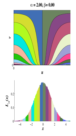
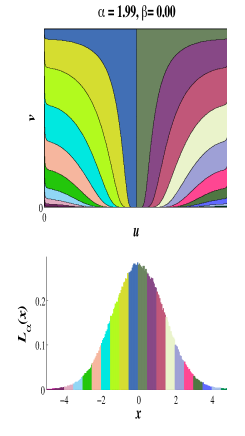
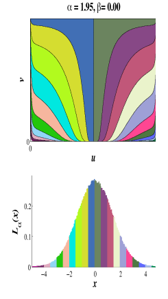
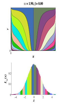
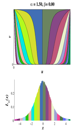
Figure 2: (Color online) The map $X=F_{\alpha}(U,V)$ with $U,V\in(0,1)$ giving the symmetric Lévy distribution $L_{\alpha}(x)$ for different values of $\alpha$. For $\alpha=2$ the picture corresponds to the Box-Muller map for the generation of Gaussian random numbers. The bottom part of each map shows the respective histogram. Areas with equal colors correspond to each other. Note that the transition from $\alpha=2$ to $\alpha<2$ is discontinuous for $u=0$ and $u=1$ and the points (0,1) and (1,1) develop a singularity.

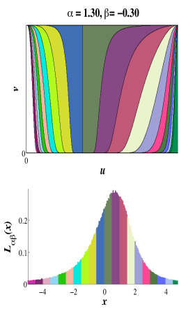
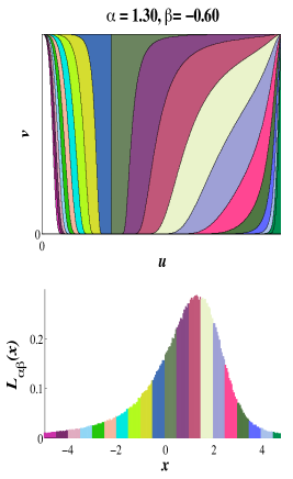
Figure 3: (Color online) The map $X=F_{\alpha\beta}(u,v)$ giving the asymmetric Lévy distribution $L_{\alpha\beta}(x)$ for two values of $\beta$.

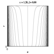
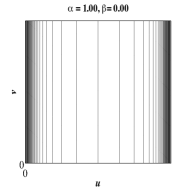
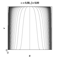
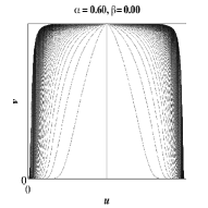
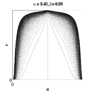
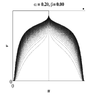
Figure 4: Isolines of the map $X=F_{\alpha}(u,v)$ with $u,v\in(0,1)$ for decreasing values of $\alpha$. The regions with increasingly divergent gradient (upper corners) is not shown beyond $|x|>600$. Note that the orientation of the isolines flips over with decreasing values of $\alpha$ at exactly $\alpha=1$.

We would like to remark that different solutions are thinkable of how to sample uniform random points in a specific region in the $(U,V)$-plane. A differential equation for the isolines can be obtained via the implicit function theorem by Ulisse Dini [6]:

$$0=\mathrm{d}F(u,v)=\frac{\partial F(u,v)}{\partial u}\mathrm{d}u+\frac{\partial F(u,v)}{\partial v}\mathrm{d}v\ ;$$ (9)

rearranging

$$\frac{\mathrm{d}v(u)}{\mathrm{d}u}=-\left(\frac{\partial F(u,v)}{\partial v}\right)^{-1}\frac{\partial F(u,v)}{\partial u}.$$ (10)

With an appropriate initial condition this differential equation defines the isoline $v(u)$ in the coordinate square spanned by $u,v$. The alternative representation of $u$ as a function of $v$ is equally appropriate from the mathematical point of view, but is less convenient in this case for symmetry reasons. We skip additional considerations on singularities and limiting behaviour. For $\alpha=2$ and $\beta=0$ Eq. (7) reduces to $X=F_{2}(U,V)=2\sqrt{-\log U}\sin(\pi(V-1/2))$, which is the Box-Muller method for Gaussian deviates with standard deviation $\sigma=\sqrt{2}$. The corresponding map is shown in the upper left of Fig. 2. The value $x$ in the condition $X>x$ determines the initial condition for Eq. (10) that determines the isoline, i.e. $x$ in the condition $X>x$, and for $\alpha=2$ it can be chosen on the boundary of the square $U,V\in(0,1)$. Two other analytic limit cases for $\beta=0$, where $L_{\alpha}(x)$ can be written in terms of elementary functions, are the Cauchy distribution, with $\alpha=1$ and $X=F_{1}(U)=\tan(\pi(U-1/2))$, and the Lévy distribution, with $\alpha=1/2$ and $X=F_{1/2}(U,V)=-\tan(\pi(V-1/2))/(2\log U\cos(\pi(V-1/2)))$. Note that for values of $\alpha\neq 2$ the map $F$ is singular in the points $(0,1)$ and $(1,1)$. In such cases the initial condition cannot be chosen on the boundary, which considerably complicates the situation numerically.

Starting from the simplest case, insertion of $F_{2}(u,v)$ into Eq. (10) yields

$$\frac{\mathrm{d}v(u)}{\mathrm{d}u}=\frac{\cot(\pi v(u))}{2\pi u\,\log(u)}.$$ (11)

Insertion of $F_{\alpha}(u,v)$ into Eq. (10) yields

$$\frac{\mathrm{d}v(u)}{\mathrm{d}u}=(\alpha-1)\left\{\frac{1}{\pi u\log(u)}\left[\tan\left(\pi\left(v(u)-\frac{1}{2}\right)(1-\alpha)\right)(\alpha-1)^{2}\right.\right.\\ \left.\left.+\cot(\pi v(u))-\alpha^{2}\cot\left(\pi\left(v(u)-\frac{1}{2}\right)\alpha\right)\right]\right\}^{-1}.$$ (12)

One way to sample directly and uniformly from the area under $v(u)$ would be an area-preserving map of a square domain spanned by two uniform random numbers, e.g. $U,V\in(0,1)$, or any other suitable two dimensional domain onto this area. To our knowledge this solution is not available yet. Alternatively, the function $v(u)$ can be obtained numerically via integration or by appropriate algorithms for the generation of isolines. Once data points for $v(u)$ are obtained, any method that samples uniformly the region $X<x$ or $X>x$ is suitable in principle. With this, the generation of a tail variable constitutes in itself a standard non-uniform variate generation task. It is the initial scenario of sampling uniformly under a curve, but with the great simplification of a finite support. However, this is not the route we propose for three reasons. First, the numerical solution of Eq. (12) is cumbersome. Second, the initial condition has to be found within the $u$-$v$ square due to the above mentioned singularities. The subsequent integration in two directions must be guaranteed to work unattended and automatically as a black box with $\alpha$ and $\beta$ as the only parameters. Third, the outcome is not exact in the sense that the sampled random tail variates are distributed with respect to an approximated probability density function based on the data point representation of the isoline. As it will turn out a numerical or analytic representation of the isoline is not a required piece of information and its calculation can be avoided. It can also be shown that the isolines are monotonic in $u$ in the regions $F_{\alpha\beta}(u,v)<0$ and $F_{\alpha\beta}(u,v)>0$ which is a useful property in Sec. 3. Although the approximation of density functions is commonly accepted as a reasonable compromise in several applications we introduce in the next section a simple graphical method without this disadvantage.

3 Sampling method and example application

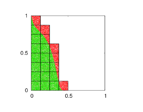
Figure 5: (Color online) Intuitive, coarsely tiled, example of the tiling in the $u$-$v$ square for sampling symmetric Lévy $\alpha$-stable random variates with the condition $X=F(u,v)<-1$ and $\alpha=1.8,\,\beta=0$. The tiled area can be sampled efficiently while only points in the red shaded region are rejected. Tiles with direct acceptance do not require the acceptance comparison $X=F(u,v)<-1$.

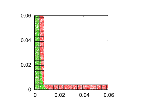
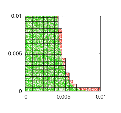
Figure 6: (Color online) Two different tiling refinements of the region corresponding to the condition $X<-12$ which is a narrow strip along the left and bottom of the unit square. Only the lower left corner is shown on a scale that magnifies the tiling to a visible size. The row of tiles on the bottom samples a narrow strip below the isoline. In the right panel the rejection rate is significantly lower. It may help intuition that the colored dots are the uniformly distributed pairs $(u,v)$.

We introduce the method using simple intuitive examples. The production algorithm relies on the rejection method whose invention dates back to von Neumann [40] and which we do not rehearse here. Fig. 5 demonstrates a computationally efficient concept for uniform sampling in a certain two-dimensional region. In the first example we aim at producing Lévy $\alpha$-stable random variates with parameters $\alpha=1.8$, $\beta=0$ and the condition $X<-1$. The map $F_{1.8}(u,v)$ for this choice of parameters is also shown in Fig. 2. It corresponds to a relatively large region in the left part of the square.

We performed a straightforward and simple tiling of this region using square tiles that can be refined, for example, iteratively maintaining complete coverage while minimizing the excess area of the tiles that stick out of the region defined by $F_{1.8}(u,v)<x$. Uniform sampling of the tiled area accepting all $X=F_{1.8}(u,v)<x$ and rejection of all other samples achieves the desired tail sampling. The size of the tiles can be chosen to achieve an arbitrarily low rejection rate. In the example shown in Fig. 5 the tiling is refined only moderately to convey the situation. For tiles that lie completely underneath the isoline the test $F_{1.8}(u,v)<x$ must not be executed. With dense tiling this comparison is therefore hardly needed and indeed must be avoided to yield a speed-up with respect to the transformation method. The setup and production loop of random variates follows the steps:

Algorithm Input: $x\in\mathbb{R}$.

0:

Setup:
Tiling of the region $F(u,v)<x$ using a method of choice.
Label tiles with an integer index.
Label tiles that are intersected by the isoline $F(u,v)=x$.

1:

Draw a random integer tile index with uniform probability.

2:

Draw a random coordinate $(u,v)$ with uniform probability within this tile.

3:

Test if the tile is intersected by the isoline (table look-up).
If yes, go to 4. If no, accept $X=F(u,v)$ and go to 1 (direct acceptance).

4:

Test if $(u,v)$ satisfies $X=F(u,v)<x$.
If yes, accept $X$, otherwise reject and go to 1.

Note that for monotonic isolines the position of a tile with respect to an isoline, i.e. whether underneath, above or intersected, can be determined by evaluating the map for at most two corners. Step 4 is unlikely to be carried out if the coverage is dense, giving nearly a zero rejection rate. Overall, this procedure is efficient in setup and production for a sufficiently dense tiling. Furthermore, with small modifications of the above acceptance and rejection conditions in the pseudo code, the tiling and production of random numbers on a finite interval $X\in[x_{1},x_{2}]$ is geometrically and algorithmically equivalent to generating numbers from the tail. This requires the tiling of a region in the $u$-$v$ square between two isolines with the condition $x_{1}<X<x_{2}$.

Fig. 6 shows the map for the left tail regions of the $u$-$v$ square with $X<-12$, which is more realistic for the purpose of tail sampling. This condition corresponds to sampling a narrow strip at the bottom and left sides of the unit square. The figure only shows the corner at the origin. The bottom strip of tiles samples an extremely narrow strip than is not visible on this scale. The iterative tile refinement in the setup stage is acceptably fast, below a second in our non-optimized code, down to the level on the right panel of Fig. 6 to achieve a rejection rate below 1%. Different values of $\alpha>0.1$ as well as not too extreme values of $x$ have no significant influence on the setup performance achieving a rejection rate of 1%. Note that the speed of random number production is independent of the number of tiles. In our case it amounts to 2.3 million tail variates per second on a PC with a 2.4 GHz Intel Pentium 4 processor using the GNU C++ compiler version 3.2.2 Linux and optimization level -O3. As the uniform random number generator we used the XOR shift SHR3 by Marsaglia [28]. The colouring of the acceptance and rejection regions in Figs. 5 and 6 are produced by green and red coloured dots representing the random uniform coordinates $(u,v)$.

We would like to stress that the method of tiling as well as the form of the tiles is in principle arbitrary. Equal size and shape is computationally advantageous, but this issue is not the focus of the present work. Of course any tiling technique that produces a similar result is suitable, using either square or rectangular tiles. However, the choice of square equal tiles is algorithmically very simple and likely to outrun an adaptive scheme with more complex shapes in setup and also production. The iterative tiling refinement, as performed in the above examples, is robust and fast also for large values of $|x|$. The rejection scheme is in principle similar to the Ziggurat implementation of Ref. [28]. It also needs the setup of a data structure that covers a region by equal area rectangles. The details of the tiling method that is more general and applicable to random number production directly via the probability density are described in separate work [7].

4 The Mittag-Leffler probability distribution

Our second example density is less know in scientific applications, even less so its transform. The Mittag-Leffler probability distribution appears e.g. in the analytic solution of the time-fractional Fokker-Planck equation [8, 12, 13, 14]. The generalized Mittag-Leffler function is defined as [11, 15]

$$E_{\alpha\beta}(z)=\sum_{n=0}^{\infty}\frac{z^{n}}{\Gamma(\alpha n+\beta)},\quad z\in\mathbb{C}.$$ (13)

For our purposes it is sufficient to restrict the example to the one-parameter Mittag-Leffler function which plays an important role in the stochastic solution of the time-fractional diffusion equation. The series representation is

$$E_{\alpha}(z)=\sum_{n=0}^{\infty}\frac{z^{n}}{\Gamma(\alpha n+1)},\quad z\in\mathbb{C},$$ (14)

leading to a pointwise representation on a finite interval. The Mittag-Leffler function with argument $z=-t^{\alpha},\ t\in\mathbb{R}$ reduces to a standard exponential decay, $e^{-t}$, with $\alpha=1$; when $0<\alpha<1$, the Mittag-Leffler function is approximated for small values of $t$ by a stretched exponential decay (Weibull function), $\exp(-t^{\alpha}/\Gamma(1+\alpha))$ and for large values of $t$ by a power law, $t^{-\alpha}/\Gamma(1-\alpha)$, see Fig. 7, top left plot. There is increasing evidence for physical phenomena [3, 30, 38, 41] and human activities [1, 35, 37] that do not follow neither exponential nor, equivalently, Poissonian statistics. The Mittag-Leffler distribution is an example of power-law distributed waiting times. They arise as the natural survival probability leading to time-fractional diffusion equations.

Eq. (14) is the complementary cumulative distribution function, also called survival function; the proability density is

$$-\frac{\mathrm{d}}{\mathrm{d}t}E_{\alpha}(-t^{\alpha}).$$ (15)

In past applications Mittag-Leffler random numbers were produced by rejection through a pointwise representation via Eq. (14), which is inefficient due to the slow convergence of the series. In some cases concepts to avoid Mittag-Leffler random numbers were presented [22, 23] due to the difficulty of their production. In this context it had not been recognized immediately that transformation formulas analogous to Eq. (7) are available [5, 9, 16, 17, 18, 19, 20, 33]. The most convenient expression is due to Kozubowski and Rachev [20]:

$$T=M_{\alpha}(U,V)=\log U\left(\frac{\sin(\alpha\pi)}{\tan(\alpha\pi V)}-\cos(\alpha\pi)\right)^{1/\alpha},$$ (16)

where $U,V\in(0,1)$ are independent uniform random numbers and $T$ is a Mittag-Leffler random number. For $\alpha=1$, Eq. (16) reduces to the transform for the exponential distribution: $M_{1}(U,V)=\log U$. Fig. 7 shows the map $M_{\alpha}(U,V)$ of the transform representation Eq. (16) as borders between intervals corresponding to $t=0,\pm 0.5,\pm 1,\pm 1.5,...$ The exponential case with $\alpha=1$ depends on only one random variable in the $u$-$v$ square which is expressed by perfectly horizontal isolines. For $\alpha<1$ the left and right edges develop singularities. It is not recommended to use Eq. (14) and summation of many terms for the computation of $E_{\alpha}(-t^{\alpha})$. A more elegant and accurate method is presented in Ref. [11, 34, 15]. For the generation of random numbers we use the implementation in Ref. [10].

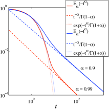
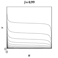
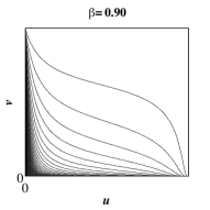
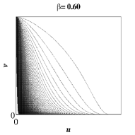
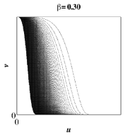
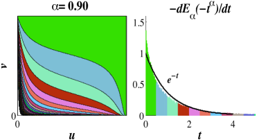
Figure 7: The Mittag-Leffler function $E_{\alpha}(-t^{\alpha})$ in a log-log plot (top left) and the transformation map $X=M_{\alpha}(U,V)$, Eq. (16), in terms of isolines for five values of $\alpha$. The case $\alpha=1$ corresponds to the standard exponential function. The regions on the left side of the maps is not shown beyond $t>600$ due to an increasingly divergent gradient. The two plots at the bottom repeat the case with $\alpha=0.9$ using colors and showing the corresponding histogram.

5 Summary and conclusion

We have demonstrated some properties of the Chambers-Mallows-Stuck and Kozubowski-Rachev transformation maps exemplifying the production of random numbers with the former. The interpretation as a two-dimensional map from the unit square to the real numbers allows to associate arbitrary intervals on the support of the density with well defined finite regions of the map domain. The uniform sampling of such regions produces directly random numbers exactly within the respective intervals. We have also introduced an efficient concept for the automatic setup of a random number generator that makes use of this property. The resulting generator can in principle produce random numbers in intervals which can be disconnected and any combination of the kind $(-\infty,x_{1}]\cup[x_{2},x_{3}]\cup\ldots\cup[x_{n},+\infty),\,x_{i}\in\mathbb{R}$. Most importantly, the sampling of tails as shown here can be used as a tail handling method in fast implementations of random number generators for which a candidate is the Ziggurat method implementation that was proven to greatly outrun simple inversion methods. The present work opens the route for the speedup of many known random number generators that rely on transform representations.

References

- [1] A.-L. Barabási, The origin of bursts and heavy tails in human dynamics, Nature 435 (2005), 207–211.
- [2] J. M. Chambers, C. L. Mallows, and B. W. Stuck, A method for simulating stable random variables, J. Amer. Statist. Assoc. 71 (1976), 340–344.
- [3] A. Clauset, C. R. Shalizi, and M. E. J. Newman, Power-law distributions in empirical data, 2007, arXiv:0706.1062 [physics.data-an].
- [4] L. Devroye, Non-uniform random variate generation, Springer, New York, 1986.
- [5] L. Devroye, Random variate generation in one line of code, Proceedings of the 1996 Winter Simulation Conference (J. M. Charnes, D. J. Morrice, D. T. Brunner, and J. J. Swain, eds.), IEEE Press, Piscataway, NJ, USA, 1996, pp. 265–272.
- [6] U. Dini, Serie di Fourier e altre rappresentazioni analitiche delle funzioni di una variabile reale, T. Nistri, Pisa, 1880.
- [7] D. Fulger and G. Germano, Automatic generation of non-uniform random variates for arbitrary pointwise computable probability densities by tiling, 2009, arXiv:0902.3088 [cs.MS].
- [8] D. Fulger, E. Scalas, and G. Germano, Monte Carlo simulation of uncoupled continuous-time random walks yielding a stochastic solution of the space-time fractional diffusion equation, Phys. Rev. E 77 (2008), 021122.
- [9] G. Germano, M. Engel, and E. Scalas, City@home: Monte Carlo derivative pricing distributed on networked computers, Proceedings of the 1st International Workshop on Grid Technology for Financial Modeling and Simulation (S. Cozzini, S. d’Addona, and R. Mantegna, eds.), 2006, PoS(GRID2006)011, http://pos.sissa.it.
- [10] G. Germano, D. Fulger, and E. Scalas, mlrnd.m: Mittag-Leffler pseudo-random number generator, 2008, Matlab Central File Exchange, file ID #19392, http://www.mathworks.com/matlabcentral/fileexchange.
- [11] R. Gorenflo, J. Loutchko, and Yu. Luchko, Computation of the Mittag-Leffler function and its derivative, Fract. Calc. Appl. Anal. 5 (2002), 491–518.
- [12] R. Gorenflo, F. Mainardi, and A. Vivoli, Continuous-time random walk and parametric subordination in fractional diffusion, Chaos Soliton Fract. 34 (2007), 87–103.
- [13] R. Gorenflo, A. Vivoli, and F. Mainardi, Discrete and continuous random walk models for space-time fractional diffusion, Nonlinear Dynam. 38 (2004), 101–116.
- [14] R. Hilfer and L. Anton, Fractional master equations and fractal time random walks, Phys. Rev. E 51 (1995), R848–R851.
- [15] R. Hilfer and H. J. Seybold, Computation of the generalized Mittag-Leffler function and its inverse in the complex plane, Integr. Transf. Spec. F. 17 (2006), 637–652.
- [16] K. Jayakumar, Mittag-Leffler process, Math. Comput. Model. 37 (2003), 1427–1434.
- [17] T. J. Kozubowski, Mixture representations of Linnik distribution revisited, Statist. Probab. Lett. 38 (1998), 157–160.
- [18] , Computer simulation of geometric stable distributions, J. Comput. Appl. Math. 116 (2000), 221–229.
- [19] , Fractional moment estimation of Linnik and Mittag-Leffler parameters, Math. Comput. Model. 34 (2001), 1023–1035.
- [20] T. J. Kozubowski and S. T. Rachev, Univariate geometric stable laws, J. Comput. Anal. Appl. 1 (1999), 177–217.
- [21] P. Lévy, Calcul des Probabilités, Gauthier–Villars, Paris, 1925.
- [22] M. Magdziarz and A. Weron, Competition between subdiffusion and Lévy flights: A Monte Carlo approach, Phys. Rev. E 75 (2007), 056702.
- [23] M. Magdziarz, A. Weron, and K. Weron, Fractional Fokker-Planck dynamics: Stochastic representation and computer simulation, Phys. Rev. E 75 (2007), 016708.
- [24] G. Marsaglia, Generating a variable from the tail of the normal distribution, Technometrics 6 (1964), 101–102.
- [25] G. Marsaglia and M. D. MacLaren, A fast procedure for generating exponential random variables, Commun. ACM 7 (1964), 298–300.
- [26] G. Marsaglia, M. D. MacLaren, and T. A. Bray, A fast procedure for generating normal random variables, Commun. ACM 7 (1964), 4–7.
- [27] G. Marsaglia and W. W. Tsang, A fast, easily implemented method for sampling from decreasing or symmetric unimodal density functions, SIAM J. Sci. Stat. Comp. 5 (1984), 349–359.
- [28] , The Ziggurat method for generating random variables, J. Stat. Software 5 (2000), 8.
- [29] Mark M. Meerschaert, David A. Benson, Hans-Peter Scheffler, and Boris Baeumer, Stochastic solution of space-time fractional diffusion equations, Phys. Rev. E 65 (2002), 041103.
- [30] M. S. Mega, P. Allegrini, P. Grigolini, V. Latora, L. Palatella, A. Rapisarda, and S. Vinciguerra, Power-law time distribution of large earthquakes, Phys. Rev. Lett. 90 (2003), 188501.
- [31] J. Nolan, Numerical calculation of stable densities and distribution functions, Commun. Statist. — Stochastic Models 13 (1997), 759–774.
- [32] , An algorithm for evaluating stable densities in Zolotarev’s (M) parametrization, Math. Comput. Modelling 29 (1999), 229–233.
- [33] A. G. Pakes, Mixture representations for symmetric generalized Linnik laws, Statist. Probab. Lett. 37 (1998), 213–221.
- [34] I. Podlubny and M. Kacenak, mlf.m: Mittag-Leffler function — Calculates the Mittag-Leffler function with desired accuracy, 2005, MATLAB Central File Exchange, file ID #8738, http://www.mathworks.com/matlabcentral/fileexchange.
- [35] M. Raberto, E. Scalas, and F. Mainardi, Waiting times and returns in high-frequency financial data: An empirical study, Physica A 314 (2002), 749–755.
- [36] H. Rubin and B. Johnson, Efficient generation of exponential and normal deviates, J. Stat. Comput. Simulation 76 (2006), 509–518.
- [37] E. Scalas, R. Gorenflo, H. Luckock, F. Mainardi, M. Mantelli, and M. Raberto, Anomalous waiting times in high-frequency financial data, Quant. Financ. 4 (2004), 695–702.
- [38] M. F. Shlesinger, G. M. Zaslavsky, and J. Klafter, Strange kinetics, Nature 363 (1993), 31–37.
- [39] D. B. Thomas, W. Luk, P. H. W. Leong, and J. D. Villasenor, Gaussian random number generators, ACM Comput. Surv. 39 (2007), 11.
- [40] J. von Neumann, Various techniques used in connection with random digits, NBS Appl. Math. Ser. 12 (1951), 36–38.
- [41] S. N. Ward, Earthquakes — a deficit vanished, Nature 394 (1998), 827–829.
- [42] R. Weron, Computationally intensive Value at Risk calculations, Handbook of Computational Statistics (J. E. Gentle, W. Haerdle, and Y. Mori, eds.), Springer, Berlin, 2004, pp. 911–950.