Adaptive gene regulatory networks

Abstract

Regulatory interactions between genes show a large amount of cross-species variability, even when the underlying functions are conserved: There are many ways to achieve the same function. Here we investigate the ability of regulatory networks to reproduce given expression levels within a simple model of gene regulation. We find an exponentially large space of regulatory networks compatible with a given set of expression levels, giving rise to an extensive entropy of networks. Typical realisations of regulatory networks are found to share a bias towards symmetric interactions, in line with empirical evidence.

The expression of genes is regulated such that the right combinations of gene products are generated at the right time and place of an organism. Key regulators of gene expression are transcription factors, proteins which bind to specific sites on DNA and influence the expression of nearby genes. Typically, the expression of a gene is effected by a combination of several transcription factors, and conversely, a transcription factor regulates several genes. Expression levels can thus depend on the entire set of regulatory interaction between transcription factors and their target genes, referred to as a regulatory network. These intracellular reaction networks process extracellular information to induce specific gene expression patterns, allowing, for instance, the development of a complex body plan, or responses to external conditions.

Even though regulatory networks are tuned carefully to produce specific expression patterns, there are in general many networks fulfilling a regulatory task. An example is the control of mating type in different yeast species: The same set of genes controlled in S. cerevisiae by an activator which is upregulated in a certain state is controlled by a repressor which is downregulated in that state in C. albicans Tsong et al. (2003). A second prominent example is the development of the anterior patterning in insect embryos, leading to the formation of the insect’s head. The gene crucial to this process in the fruit fly Drosophila, called bicoid, is absent in many other insects, where a combination of different genes take on the same task Schröder (2003). Even whole sets of genes which are co-expressed across the entire yeast family can have different regulatory interactions in different species Tanay et al. (2005). Source of these changing interactions is a rapid evolutionary turnover of transcription factor binding sites at the level of DNA sequences Tautz (2000); Mustonen and Lässig (2005). This can generate new regulatory interactions. A recent essay on the degeneracy of regulatory networks can be found in Chouard (2008).

The large number of regulatory networks with a given function (viable networks) is particularly relevant from an evolutionary perspective, as neutral evolution gradually explores different viable networks. Viable networks can form a set with intricate geometric features in the space of regulatory network. An analogy is the set of all RNA-sequences which fold into a given secondary structure, which stretches across the entire sequence space Schuster et al. (1994). Numerical studies, based on simple models of gene regulation Bornholdt and Sneppen (1998) found that the space of viable networks can be crossed in small steps, and that a wide range of new expression patterns can be generated by small changes to different viable networks Ciliberti et al. (2007a, b).

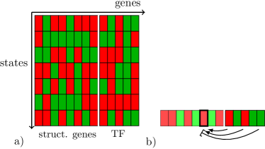
Figure 1: Expression levels and regulatory networks. a) We list genes along the $x$-axis, and states of the organism along the $y$-axis. Following established convention in expression analysis, expression levels are colour-coded with high expression levels shown in red (dark), low levels in green (light). b) Regulatory interactions must be compatible with gene expression levels in all states of the organism. The schematic example shows interactions between transcription factors and a single target gene; two enhancing interactions ($\rightarrow$) with upregulated transcription factors, and a repressive interaction ($\dashv$) with a downregulated transcription factor lead to the activation of the target gene.

These observations call for a statistical approach based on the ensemble of all viable networks, which is the topic of this paper. We consider a model with two classes of genes: structural genes (coding e.g. for enzymes or cellular components), and transcription factors. The expression levels of structural genes are prescribed for different states of the organism and are fixed for a given state. For instance, when nutrients are available, specific enzymes have to be produced to digest these nutrients. On the other hand, the expression levels of transcription factors, and the regulatory interactions between genes can be adapted to meet the expression levels of structural genes. The freedom to alter expression levels of transcription factors turns out to be crucial.

In the following, we develop a simple model based on quenched random expression levels of structural genes, and adaptive regulatory interactions and expression levels of transcription factors. The ensemble of viable networks is characterized by the microcanonical partition function

$$Z\equiv e^{S}=\frac{\mbox{Tr}_{{\bf J},{\bf\xi}_{t}}I({\bf J},{\bf\xi})}{\mbox{Tr}_{{\bf J},{\bf\xi}_{t}}}\ ,$$ (1)

giving the fraction of viable networks in terms of the trace $\mbox{Tr}_{{\bf J},{\bf\xi}_{t}}$ over the phase space (regulatory interactions ${\bf J}$ and the expression levels of transcription factors ${\bf\xi}_{t}$) and an indicator function $I({\bf J},{\bf\xi})$ of couplings and all expression levels. The indicator function is defined to equal one for a viable network and zero otherwise.

Specifically, genes are labelled $i=1,\ldots,N$ for structural genes and $i=N+1,\ldots,\beta N$ for transcription factors. The regulatory network is encoded in a matrix of regulatory interactions $J_{ij}$, with positive $J_{ij}$ indicating that gene $j>N$ produces a transcription factor which enhances the expression of gene $i\neq j$, and represses gene $i$ for negative values of $J_{ij}$. Different external and internal states of the organism are labelled by $\mu=1,\ldots,\alpha N$. $\xi_{i}^{\mu}$ denotes the (log-)expression level of gene $i$ in state $\mu$, and is positive for high concentrations of the gene product and negative for low concentrations. Assuming transcription factors act independently on their target genes, the condition for a viable network is modelled as

$$\xi_{i}^{\mu}/\sqrt{N}\sum_{j}J_{ij}\xi_{j}^{\mu}>\kappa\ \ \ \forall i,\mu\ .$$ (2)

Threshold condition (2) has been used extensively to model neural J.Hertz et al. (1991) and gene regulatory networks Wahde and Hertz (2000); Buchler et al. (2003); Ciliberti et al. (2007a, b). The indicator function for a viable network in the partition function (1) can be written in terms of the Heaviside step-function $\Theta(x)$ as

$$I(\{J_{ij},\xi_{i}^{\mu}\})\!\! = \!\!\prod_{i,\mu}\Theta\left(\frac{1}{\sqrt{N}}\xi_{i}^{\mu}\sum_{j}J_{ij}\xi_{j}^{\mu}-\kappa\right)$$

$$= \!\!\prod_{i,\mu}\int_{\kappa}^{\infty}\!\!\!d\lambda\int\!\frac{dx}{2\pi}e^{i\sum_{i\mu}\lambda_{i}^{\mu}x_{i}^{\mu}-\frac{i}{\sqrt{N}}\sum_{ij\mu}x_{i}^{\mu}\xi_{i}^{\mu}J_{ij}\xi_{j}^{\mu}}.$$

We constrain vectors of regulatory interactions ${\bf J}_{i}$ and of expression levels ${\bf\xi}_{i}$ to lie on hyperspheres. This defines the trace over phase space (4)

$$\mbox{Tr}=\prod_{i}\int d\mu({\bf J}_{i})\prod_{i>N}\int d\mu({\bf\xi}_{i})$$ (4)

with $d\mu({\bf J}_{i})=\prod_{j>N}dJ_{ij}\delta\left((\beta\!-\!1)N-\sum_{j>N}J_{ij}^{2}\right)$ and analogously for the transcription factor expression levels. The quenched average of (1) over expression levels of structural genes $\langle\langle\ln Z\rangle\rangle=\prod_{i\leq N}\int d\mu({\bf\xi}_{i})\ln Z$ is performed using the replica trick.

Figure 2: Averaging over expression levels. a) The diagrams corresponding to the first three terms in (Adaptive gene regulatory networks) are shown along with their combinatorial factors. Nodes represent variables $i,j,\ldots$, solid lines indicate the corresponding matrix entries $G_{ij}$, dashed lines are contractions $i=j$. b) Plotting the logarithm of (Adaptive gene regulatory networks) against $\gamma$ shows the contribution of different diagrams. The first diagram gives a linear term (thin solid line), the series up to second and third order are shown by the dashed and dashed-dotted curves respectively. These are valid approximations up to some finite values of $\gamma$ only. The thick solid line gives the full series to infinite order (thick solid line) along with a numerical computation of (Adaptive gene regulatory networks), where $G_{ij}$ was taken a random matrix of size $N=50$ with i.i.d. normally distributed elements.

Transcription factors play a special role; their expression levels provide the regulatory input for every gene in the regulatory network. This produces an effective coupling between regulatory interactions of different genes. One consequence emerges already at the level of the average of (Adaptive gene regulatory networks) over the expression levels $\xi$. As an illustration, we consider a toy problem, where the average of $\exp\{-i\sqrt{\gamma/(2N)}\sum_{ij}\xi_{i}G_{ij}\xi_{j}\}$ is computed over a distribution of independent normally distributed variables $\xi_{i}$. $G_{ij}$ is a symmetric matrix with uncorrelated random entries.

$$\langle e^{-\frac{i}{2}\sqrt{\gamma/N}\sum_{ij}\xi_{i}G_{ij}\xi_{j}}\rangle=1/\sqrt{\det(\leavevmode\hbox{\small 1\kern-3.3pt\normalsize 1}+i\sqrt{\gamma/N}{\bf G})}$$

$$= \exp\{-\frac{1}{2}\sum_{n=1}^{\infty}\frac{1}{n}\mbox{tr}(i\sqrt{\gamma/N}{\bf G})^{n}\}$$

$$= \exp\{\gamma/4\sum_{i}z_{i}-\gamma^{2}/4\sum_{i}z_{i}^{2}+5\gamma^{3}/12\sum_{i}z_{i}^{3}+\cdots\}$$

$$= \exp\{\sum_{i}w(\gamma z_{i})\}$$

with shorthand $z_{i}=1/N\sum_{j}G_{ij}G_{ji}$ and tr denoting the matrix trace. The successive terms in the power series (Adaptive gene regulatory networks) can be represented diagrammatically; Fig. 2 a) shows the first three diagrams. Fig. 2 b) shows how the different powers in (Adaptive gene regulatory networks) contribute to the average and how for finite values of $\gamma$ the series has to be taken to infinite order, giving $w(z)=\frac{2z+1-\sqrt{1+4z}}{8z}-\frac{1}{2}\log\left(\frac{1}{2}+\frac{1}{2}\sqrt{1+4z}\right)$. This is in contrast to the standard situation in fully-connected disordered models, where in the thermodynamic limit the series in (Adaptive gene regulatory networks) terminates after the first term.

The approach (Adaptive gene regulatory networks) applied to the full model (1)-(Adaptive gene regulatory networks) gives $\sum_{i\leq N,\mu}w(z_{i}^{\mu})+\sum_{i>N,\mu,a}w(z_{i}^{\mu a})$ with $z_{i}^{\mu}=\sum_{a}(x_{i}^{\mu a})^{2}$ and $z_{i}^{\mu a}=(x_{i}^{\mu a})^{2}+\frac{1}{N}\sum_{j}(x_{i}^{\mu a})^{2}(J_{ji}^{a})^{2}+\frac{2}{N}\sum_{j}x_{i}^{\mu a}x_{j}^{\mu a}J_{ij}^{a}J_{ji}^{a}$. Neglecting fluctuations of $z_{i}^{\mu a}$ across genes, the entropy of viable networks $\langle\langle S\rangle\rangle\equiv N^{2}s$ can be computed in the thermodynamic limit $N\to\infty$ by standard methods. Within a replica-symmetric ansatz we obtain

$$s=\mbox{extr}\left[\frac{1}{2}\alpha(\beta\!-\!1)\!\left(F-\ln F\right)+\frac{1}{2}\alpha\hat{X}_{2}^{-}X_{2}^{-}\right.$$ (6)

$$\left.+\frac{1}{2}\alpha(\beta\!-\!1)\hat{X}_{2}^{+}X_{2}^{+}+\alpha(\beta\!-\!1)\hat{X}_{1}X_{1}+\frac{(\beta\!-\!1)^{2}}{4}\ln\left(1-h^{2}\right)\right.$$

$$\left.+\alpha(\beta\!-\!1)\ln\left[\int_{\kappa}^{\infty}d\lambda\int\frac{dx}{2\pi}\exp\left\{w\left(\frac{1}{F^{2}}\left[x^{2}+X_{2}^{+}\right.\right.\right.\right.\right.$$

$$\left.\left.\left.\left.\left.-2ixhX_{1}\right]+\frac{X_{2}^{-}}{(\beta\!-\!1)F}\right)+i(\lambda-\hat{X}_{1})x-\frac{1}{2}\hat{X}_{2}^{+}x^{2}\right\}\right]\right.$$

$$\left.+\alpha\int d\hat{y}dye^{\left[iy\hat{y}+w\left(\frac{y}{F}\right)\right]}\ln\left[H\left(\frac{\kappa}{\sqrt{\hat{X}_{2}^{-}+2iy}}\right)\right]\right]\ .$$

The entropy $s$ of viable networks is determined by the extremum over the saddle point parameters $F,X_{1},\hat{X}_{1},X_{2}^{\pm},\hat{X}_{2}^{\pm}$, and $h$. Saddle point parameter $h$ has an intuitive interpretation in terms of the symmetry of regulatory interactions and will be discussed below. $H(x)$ denotes the cumulative Gaussian measure $\int_{x}^{\infty}\!\!\frac{dy}{\sqrt{2\pi}}\exp\{-y^{2}/2\}$.

The entropy of viable networks (6) decreases with increasing number of patterns $P=\alpha N$, see Fig. 3. This is to be expected, as each set of expression patterns induces a new set of constraints on the network. However, the entropy remains finite even as the number of patterns becomes large with $\alpha\to\infty$: there (typically) always exists a viable network, and there is no transition to a phase where solutions of (2) no longer exist. Such phase transitions are well known in neural networks and many combinatorial problems J.Hertz et al. (1991). In contrast, the ability of regulatory networks to store a large number of expression patterns of structural genes stems directly from the freedom to choose expression levels of transcription factors: transcription factor expression levels adapt in such a way that regulatory interactions compatible with expression levels of all genes can be found.

The saddle point parameter $h=\frac{1}{(\beta\!-\!1)^{2}N^{2}}\sum_{i,j}J_{ij}J_{ji}$ is the symmetry parameter of the resulting regulatory network. A positive value of $h$ indicates that if gene $i$ regulates gene $j$, and also $j$ regulates $i$, the signs of these interactions are correlated, with like signs occurring more frequently than opposite signs. The origin of this symmetry lies in condition (2) for a viable network, where a positive value of $\xi^{\mu}_{i}\xi^{\mu}_{j}$ for some $i,j,\mu$ gives rise to positive values for both $J_{ij}$ and $J_{ji}$, and analogously for negative values. Thus the symmetry parameter $h$ increases with the number of expression patterns; Fig. 3 shows the analytical result for $h$ along with the outcome of numerical simulations.

This statistical bias towards symmetric interactions is compatible with empirical data on regulatory networks. A literature search for well-documented cases of mutually interacting genes with known interaction sign finds $9$ cases of mutually interacting gene pairs with like interaction sign symmetric compared to only $3$ cases with different sign asymmetric . A nontrivial statistics of reciprocal interactions has also been found in neural and metabolic networks Garlaschelli and Loffredo (2004), where, however, the signs of the interactions are generally unknown.

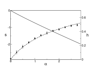
Figure 3: Entropy and symmetry of viable networks. With increasing number of patterns $P=\alpha N$, the space of viable networks shrinks, and the networks become increasingly symmetric, see text. Here the entropy $s$ per structural gene (solid line) and symmetry parameter $h$ (dashed line) are plotted against $\alpha$ for $\beta=2,\kappa=0$. The $\blacksquare$-symbols stem from numerical simulations with $N=80$, averaged over $20$ realizations of the quenched disorder (mean and standard error). The numerics is based on simulated annealing under Monte-Carlo dynamics of the regulatory interactions $J_{ij}$ and the expression levels of transcription factors $\xi^{\mu}_{i>N}$.

Over long evolutionary timescales, the required expression levels of structural genes can change. In the case of enzymes, for instance, changing nutrient availability or changing metabolic rates alter the required expression levels. Such changes of the expression levels of structural genes induce adaptive changes both of the regulatory network, and of the expression levels of transcription factors. To investigate the adaptation to changing expression levels of structural genes, we systematically perturb the expression levels of structural genes of a viable network, rendering it, in general, at first unviable. (Expression levels $\xi_{i\leq N}^{\mu}$ are perturbed by adding i.i.d. Gaussian random variables with mean zero and standard deviation $\eta$ and normalizing their variances to one again.) Subsequently, regulatory interactions and transcription factor expression levels are adapted until the viability condition (2) is satisfied again. The overlap $q_{\xi}^{<}=\frac{1}{NP}\sum_{i\leq N,\mu}\xi_{i}^{\mu}\xi_{i}^{\prime\mu}$ of structural gene expression levels of the unperturbed (unprimed) and the perturbed (primed) system quantifies the strength of the perturbation, the analogously defined $q_{\xi}^{>},q_{J}^{<},q_{J}^{>}$ quantify the response of the system to this perturbation. Figure 4 shows the overlaps as a function of perturbation strength. One finds that already small perturbations with $q_{\xi}^{<}\approx 1$ result in a drop of the overlaps to a plateau value. Larger perturbations, and even the limit $q_{\xi}^{<}\to 0$ induce only a slow decay of $q_{\xi}^{>},q_{J}^{<},q_{J}^{>}$ from their plateau values. Accordingly, close to any viable network for one set of expression levels of structural genes, there exists a viable network for any other, even unrelated set of expression levels. This effect allows fast adaptation to changes in the required expression levels.

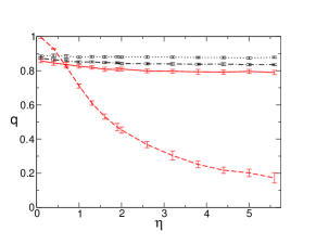
Figure 4: Response to changing expression levels. The overlaps of perturbed and unperturbed systems (see text) are plotted against the perturbation strength $\eta$: structural genes expression level overlaps (red dashed line) tend to zero with increasing $\eta$ by construction, whereas TF expression level overlaps (red solid line) quickly reach a plateau. The same holds for regulatory interactions to TF (black dotted line), and interactions to structural genes (black dash-dotted). The plateau value decreases with the fraction $1-\beta$ of TF in the genome. The data stem from Monte-Carlo simulations with $N=40$, $\alpha=1$, $\beta=2$, and $\kappa=0$, averaged over $20$ samples.

Another consequence of the observed drop of the TF expression level overlap to a plateau is that expression levels of TF change more than those of structural genes for small perturbations. For large perturbations, the expression levels of TF change less than those of structural genes. This effect may explain an apparent contradiction in the cross-species comparison of experimentally measured expression levels. A comparison of humans with other primates shows large changes of TF expression levels Gilad et al. (2006) compared to structural genes, different Drosophila species show only small changes of TF expression levels compared to structural genes Rifkin et al. (2003).

In summary, we have investigated the degeneracy of regulatory networks within a simple model of genetic regulation. Whereas the connection between annealed TF expression levels and the large space of viable networks is likely to persist also in more complex models, the geometry of this space may well change. In particular, models taking into account physical interactions between transcription factors to implement logical functions Buchler et al. (2003) lead to p-spin interactions $J_{ijk\ldots}$ and may result in a disconnected solution space and combinatorial complexity.