polymake and Lattice Polytopes

Abstract.

The polymake software system deals with convex polytopes and related objects from geometric combinatorics. This note reports on a new implementation of a subclass for lattice polytopes. The features displayed are enabled by recent changes to the polymake core, which will be discussed briefly.

1. Introduction

polymake is a software system designed for analyzing convex polytopes, finite simplicial complexes, graphs, and other objects. While the system exists for more than a decade [14] it was continuously developed and expanded. The most recent version fundamentally changes the way to interact with the system. It now offers an interface which looks similar to many computer algebra systems. However, on the technical level polymake differs from most mathematical software systems: rule based computations and an extendible dual Perl/C++ interface are the most important characteristics.

polymake can now also handle hierarchies of objects where each level may come with additional sets of rules. polymake handles casts between subclasses based on property requests. We will explain this feature by means of a new subclass LatticePolytope that is derived from the existing class Polytope<Rational>. However, some of the new functions can also be applied to any rational polytope. A lattice polytope is a polytope whose vertices are contained in a lattice $\Lambda\subset{\mathbb{R}}^{n}$ [6, 2]. polymake always assumes $\Lambda={\mathbb{Z}}^{n}$. This subclass reflects a new use of polymake in toric geometry, where lattice polytopes encode properties of toric varieties and toric ideals [21, 12]. String theorists have been interested in special lattice polytopes, as they led to the construction of mirror pairs of Calabi-Yau varieties [4]. Gröbner bases of toric ideals have been applied to optimization problems [27].

We will explain all relevant concepts for our exposition on the way. Lattice polytopes have also become an important subject in other areas of mathematics. Enumerating non-negative solutions of Diophantine equations can be interpreted as counting lattice points in a polyhedron [25]. Contingency tables in statistics can be modeled by lattice polytopes [11]. Sampling then corresponds to finding integral points in the polytope.

The paper is organized as follows. First we will review the recent changes and the new polymake interface. Then we will report on our new implementation of a subclass for lattice polytopes. In particular, this comprises interfaces to 4ti2 [1], Latte macchiato [10, 16], and normaliz2 [8]. We will show how the user can benefit from the common interface to these systems via polymake and how one can extend their functionality by combining with polymake’s features. Rather than discussing implementation details we will explain the functions available with one easy running example. This note then concludes with a final section analyzing a specific $6$-dimensional polyhedral cone which was found to be a counter-example to a conjecture of Sebő [23] by Bruns et al. [7].

2. polymake – the Next Generation

The general ideas which lead to the design and the implementation of the polymake system more than ten years ago are still valid. The key goals are the following.

• The system should be scalable with the user’s ability to write programs. This means that basic usage should not require any programming skills, while it should be powerful enough not to restrain the programming expert.

• The system should not try to “re-invent the wheel”. There is a multitude of valuable pieces of software for individual tasks; so they should be suitably interfaced rather than their functionality be duplicated.

• The system should be really easy to extend. It should be possible to model new mathematical objects and to integrate them into the existing framework.

These “golden rules” are most natural, and most users of mathematical software systems would probably agree that all of these are very desirable. For instance, the SAGE system is following a similar strategy albeit on a somewhat larger scale [26]. In polymake we are focusing on convex polytopes and related objects from the realm of geometric combinatorics. The “golden rules” already have a number of implications, some obvious and some less obvious. The most important design decisions which can be derived are: The system requires both a compiled and an interpreted programming language (we settled for C++ and Perl), and the system must be an Open Source project (we settled for the GNU Public License). By far the most difficult to accomplish is the third rule. And, in fact, a large part of polymake’s code evolution over the last decade can be seen as an attempt to re-interpret this rule again and again with an increasing level of abstraction.

A word of warning to the experienced polymake user. On a technical level the new version of polymake is very different from previous versions. From the point of view of the working mathematician this results in a number of benefits. In particular, the overall usability is improved, while we gained additional flexibility and speed. The unavoidable drawback is that the interface had to be changed in a substantial way.

Using polymake now means to start a program named “polymake” from the command line, and then to work in a shell-type environment typical for most computer algebra systems. The language for interacting with the system is Perl, but we added a few features in order to easy the usability. We give a very brief overview of how to get started with the new system.

Welcome to polymake version 2.9.6, rev. 9033
Copyright (c) 1997-2009
Ewgenij Gawrilow (TU Berlin), Michael Joswig (TU Darmstadt)
http://www.math.tu-berlin.de/polymake,  mailto:polymake@math.tu-berlin.de

This is free software licensed under GPL; see the source for copying conditions.
There is NO warranty; not even for MERCHANTABILITY or FITNESS FOR A PARTICULAR PURPOSE.

Type ’help;’ for basic instructions.

Application polytope uses following third-party software (for details: help ’credits’;)
4ti2, azove, cddlib, lrslib, nauty, normaliz2, porta, qhull, splitstree, topcom, vinci
polytope >

By now there are several different applications known to polymake. Each application comprises a main object type, properties which describe an object of this type, and a set of rules. By default the first application to start is the one dealing with convex polytopes, and this is made visible by showing the command line prompt “polytope >”. The last line before the prompt lists the programs whose interfaces are loaded. Since everything (the application, the objects, the properties, the rules, the interfaces, and the defaults) can be modified or extended by the user, what shows up exactly very much depends on the local installation. The main purpose of this note is to explain how a new sub-type for lattice polytopes is organized within the object hierarchy for general polytopes.

The following simple example can explain the polymake concept in a nutshell. The first command produces a $3$-dimensional cube with $\pm 1$-coordinates (and assigns it to the variable $P), while the second one (separated by “;”) prints its $f$-vector, that is, the number of faces per dimension. Clearly we have eight vertices, 12 edges, and six facets.

polytope > $P=cube(3); print $P->F_VECTOR;
8 12 6

The function cube returns a polytope object of type Polytope<Rational>, and F_VECTOR is a property of this class, which models polytopes with rational coordinates. Notice that there are polytopes whose combinatorial type does not admit any rational representation [28, §6.5]. polymake reduces computing the $f$-vector of this cube to finding a suitable sequence of rules and to execute them one after another. These rules can be shown as follows. To this end we restart from scratch.

polytope > $P=cube(3); print join(", ", $P->list_properties);
AMBIENT_DIM, DIM, FACETS, VERTICES_IN_FACETS, BOUNDED
polytope > print $P->type->full_name;
Polytope<Rational>

Our cube $P is “born” as an object with the five initial properties AMBIENT_DIM, DIM, FACETS, VERTICES_IN_FACETS, BOUNDED, all of which are redundant except for FACETS, which gives a description of the cube as the intersection of six affine halfspaces.

polytope > print $P->FACETS;
1 1 0 0
1 0 0 1
1 0 1 0
1 0 -1 0
1 -1 0 0
1 0 0 -1

Each line is a vector $(\alpha_{0},\alpha_{1},\dots,\alpha_{d})$ representing the linear inequality $\alpha_{0}+\alpha_{1}x_{1}+\dots+\alpha_{d}x_{d}\geq 0$. The property AMBIENT_DIM, for instance, is the dimension of the space where our polytope lives in, that is the number $d$, which can easily be derived from each facet by counting the number of columns. Now, asking for the $f$-vector means that it has to be computed from the data given somehow. We can look at the schedule of rules necessary to accomplish this task.

polytope > $schedule=$P->get_schedule("F_VECTOR");
polytope > print join("\n", $schedule->list);
HASSE_DIAGRAM : VERTICES_IN_FACETS
F_VECTOR, F2_VECTOR : HASSE_DIAGRAM

Each line is one rule. Each rule has its targets to the left of the “:” and its sources to the right. The first line says: “I can produce the Hasse diagram (of the face lattice) if I know which vertex is incident with which facet”. This is clear since it follows from the facet that the face lattice is co-atomic, that is, each face is the intersection of facets [28, §2.2 ]. The second line says: “I know how to compute the $f$-vector (and something else that we do not care to discuss now) from the Hasse diagram. Each rule comes with a piece of (Perl) code which actually implements what the rule heads shown promise. The schedule is an object of its own right, and it can be applied to the cube, which means that the corresponding Perl code is executed in the order of the schedule.

polytope > $schedule->apply($P);
polytope > print join(", ", $P->list_properties);
AMBIENT_DIM, DIM, FACETS, VERTICES_IN_FACETS, BOUNDED, HASSE_DIAGRAM, F_VECTOR,
F2_VECTOR

We see that the list of properties known about our cube changed. Three new properties have been added, and these correspond to the total of three targets of the two rules above. If we now ask for the $f$-vector this information is already stored with the cube object, and it is read from memory rather than re-computed.

As far as technology is concerned, the function cube which was called to produce the cube is written in C++. On top of the standard Perl-interface to C we built a shared memory mechanism to access an object from the C++ and the Perl side. This is also fully extendible, which means that the user is welcome to add new functions to produce other polytopes, new properties of polytopes, or new rules to compute existing properties in a different way. The integration of new functions, properties, and rules is seamless, that is, they cannot be distinguished from the built-in ones.

There are many more things to be said about this concept both from the logical and the technical point of view, but for the details we refer the reader to [14] and to further documentation at http://www.opt.tu-darmstadt.de/polymake.

3. Lattice Polytopes as a Subclass

The new version of polymake can now handle derived classes of objects specified by some preconditions that inherit all properties and rules from their base class but may provide additional rules that are specific for their class. A user may, but doesn’t have to, specify, that the object he defines falls in this class. polymake decides upon what properties a user asks for, whether the object should be cast into this subclass. Of course, before performing the cast, polymake checks whether the object meets the requirements for the subclass. The first occurrence of this new mechanism is in the class LatticePolytope derived from Polytope<Rational>. In polymake, a lattice polytope is a bounded rational polytope whose vertices are in the integer lattice ${\mathbb{Z}}^{n}$. The new rules in this object class concern properties of such polytopes in connection with toric algebra and algebraic geometry.

The main focus of our implementation concerning lattice polytopes is toric geometry, so we explain this connection here. Let $P$ be a lattice polytope. The normal fan ${\mathscr{N}}_{P}$ defines a projective toric variety $X_{P}$ [12, 27]. The defining ideal ${\mathscr{I}}_{P}$ of $X_{p}$ is a homogeneous toric ideal. Many properties of the variety are reflected in the corresponding polytope. We will see some entries in this “dictionary” which translates back and forth below.

There are several software packages available which proved to be useful in applications in this area. normaliz2 by Bruns and Ichim [8] computes Hilbert bases and $h^{*}$-polynomials. Latte macchiato by Köppe [16] builds on previous work by De Loera et al. [10], and its key application is to count lattice points and to compute Ehrhart polynomials. 4ti2 by Hemmecke et. al. [1] solves integral equations over ${\mathbb{Z}}$ and it computes convex hulls as well as Hilbert bases. polymake now provides a unified access to these programs. Additionally, we implemented various rules to compute further important properties of lattice polytopes which can be derived. We will browse through the main features by using the $3$-cube from above as our running example. As already mentioned, our cube is the convex hull of all $\pm 1$-vectors, so the vertices do lie in the ${\mathbb{Z}}^{3}$-lattice. We can let polymake check this for us.

polytope > print $P->LATTICE;
1

Here the output “$1$” represents the boolean value “true”. For instance, we can ask for the number of lattice points contained in the cube, that is, for the number $|[-1,1]^{3}\cap{\mathbb{Z}}^{3}|$. In our case, we should obtain “$27$” as the answer, there is exactly one lattice point contained in the relative interior of each non-empty face.

polytope > print $P->N_LATTICE_POINTS;
polymake: used package latte
 LattE macchiato is an improved version of LattE, a free software dedicated
 to the problems of counting and detecting lattice points inside convex polytopes,
 and the solution of integer programs.
 Copyright by Matthias Koeppe, Jesus A. De Loera and others.
 http://www.math.ucdavis.edu/~mkoeppe/latte/

27

As shown Latte macchiato was called for the computation. It uses an enhanced version of Barvinok’s algorithm[17, 3]. By default polymake gives credit to a program when it calls it for the first time. The corresponding output is omitted in some of the computations below; but we will explain which package was called in each case.

polytope > print $P->N_INTERIOR_LATTICE_POINTS;
1

Sometimes it is important to know how many of the lattice points in a polytope are contained in the interior. While the Barvinok algorithm avoids to enumerate the points, the user can force the complete enumeration. This will be computed by 4ti2.

print $P->INTERIOR_LATTICE_POINTS;
1 0 0 0

Up to this point, none of the rules used was specific to lattice polytopes. To the contrary, all this makes perfect sense for any rational polytope.

Let us now switch to some properties that are only defined for lattice polytopes. A lattice polytope is reflexive, if the origin is in the interior of the polytope and all facets have integral distance one from the origin. Equivalently, a lattice polytope is reflexive, if also its polar is a lattice polytope. In algebraic geometry, these polytopes correspond to Gorenstein toric Fano varieties. These polytopes were introduced by Batyrev [4] to construct mirror pairs of Calabi-Yau varieties in the context of string theory. A necessary condition for a polytope to be reflexive is, that the origin is the unique interior lattice point, so the cube is a candidate.

polytope > print $P->REFLEXIVE;
1

Of course, this is not a surprise, as the polar dual of the cube (with $\pm 1$-coordinates) is the regular octahedron, the convex hull of the standard basis vectors and their negatives. Reflexivity is a property that is only defined for lattice polytopes, and so at this point, polymake has internally cast the cube to the subclass LatticePolytope.

polytope > print $P->type->full_name;
LatticePolytope

Notice the difference to the first call of the same command at the very beginning. Many further properties of Fano varieties can be checked via the corresponding polytope. Reflexive polyhedra have been classified in dimensions up to $4$, see [18]. In dimension $3$, there are $124$ of these, of which $18$ correspond to smooth Fano varieties. The toric variety $X_{P}$ is smooth (or non-singular) if every cone in the normal fan ${\mathscr{N}}_{P}$ is unimodular. A cone is unimodular, if its minimal integral generators can be extended to a basis of ${\mathbb{Z}}^{n}$.

polytope > print $P->SMOOTH;
1

We will now explore a different aspect of lattice polytopes. Stanley showed [24] that for any $d$-dimensional polytope $P$ there is a polynomial $h^{*}\in{\mathbb{Z}}[t]$ of degree at most $d$ with non-negative coefficients such that

$$\sum_{k\geq 0}|kP\cap{\mathbb{Z}}^{d}|t^{k}\ =\ \frac{h^{*}(t)}{(1-t)^{d+1}}\,.$$

The polynomial $h^{*}(t)=\sum_{k=0}^{d}h^{*}_{k}t^{k}$ is the $h^{*}$-polynomial of $P$. It is closely related to the Ehrhart polynomial. Some of the coefficients have a combinatorial meaning. For instance, $h_{d}^{*}$ counts the number of interior lattice points, while the sum of all coefficients is the normalized volume of the polytope. The normalized volume of a $d$-dimensional polytope is $d!$ times the $d$-dimensional Euclidean volume. We can compute the coefficients for the cube (starting with the constant coefficient).

polytope > print $P->H_STAR_VECTOR;
1 23 23 1
polytope > print $P->LATTICE_VOLUME;
48

polymake calls normaliz2 to compute this. The degree $\delta$ of $P$ is defined as the degree of the $h^{*}$-polynomial.

polytope > print $P->LATTICE_DEGREE;
3

The value $d+1-\delta$ is the smallest factor by which we have to dilate $P$ so that it has an interior lattice point. This is the co-degree of the polytope. polymake computes it with the command LATTICE_CODEGREE. In our case, this gives $1$, as the cube contains the origin. Recent results suggest that the degree is a more relevant invariant of a lattice polytope than the dimension. For instance, it is known that for given degree $d$ and normalized volume $V$ or linear coefficient $h_{1}^{*}$ there is a constant $c$ such that any lattice polytope of dimension $d\geq c$ is a lattice pyramid (a pyramid where the apex is a lattice point with height $1$ over the base) [5, 20]. The $h^{*}$-polynomials of a lattice polytope $P$ and the lattice pyramid with base $P$ coincide.

Finally, we can use polymake to draw our cube, together with its lattice points. By default the command

polytope > $P->VISUAL->LATTICE_COLORED;

triggers the visualization with JavaView [22]. See Figure 1.

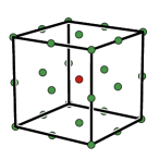
Figure 1. The $3$-dimensional cube with its lattice points. The interior lattice points are drawn in a different color.

4. Analyzing an Example

Let us look at the cone $C\subset{\mathbb{R}}^{6}$ positively spanned by the rows of the $10\times 6$-matrix

$$M\ =\ \begin{pmatrix}0&1&0&0&0&0\\ 0&0&1&0&0&0\\ 0&0&0&1&0&0\\ 0&0&0&0&1&0\\ 0&0&0&0&0&1\\ 1&0&2&1&1&2\\ 1&2&0&2&1&1\\ 1&1&2&0&2&1\\ 1&1&1&2&0&2\\ 1&2&1&1&2&0\end{pmatrix}\,.$$ (1)

The cone $C$ is pointed, that is, it does not contain any line. Equivalently, $C$ is projectively equivalent to a polytope $\bar{C}$. The rows of $M$ are precisely the rays (or generators) of $C$, that is, they correspond to the vertices of $\bar{C}$. The key fact about $C$ is the following.

Theorem 1 (Bruns et al. [7]).

The vector $(9,13,13,13,13,13)$ lies in $C$, but it cannot be written as a non-negative integral linear combination of six generators of $C$.

This says that $C$ does not satisfy the integral Carathéodory property, and thus it is a counter-example to a conjecture of Sebő [23]. We will sketch how this can be verified using polymake. Moreover, we will reveal the combinatorial structure. There is an integral transformation which maps $C$ to a cone with $0/1$-coordinates [7], and there is also a realization of $\bar{C}$ as a lattice polytope. Both other representations could be used in the sequel with the same results. The following command creates a new matrix object representing the matrix $M$ above. Here the user types in the coefficient directly; alternatively, they could also be read from a file.

polytope > $M=new Matrix<Rational>(<<".");
polytope (2)> 0 1 0 0 0 0
polytope (3)> 0 0 1 0 0 0
polytope (4)> 0 0 0 1 0 0
polytope (5)> 0 0 0 0 1 0
polytope (6)> 0 0 0 0 0 1
polytope (7)> 1 0 2 1 1 2
polytope (8)> 1 2 0 2 1 1
polytope (9)> 1 1 2 0 2 1
polytope (10)> 1 1 1 2 0 2
polytope (11)> 1 2 1 1 2 0
polytope (12)> .

polymake can work with pointed polyhedral cones right away, so it is legal to write

polytope > $C=new Polytope<Rational>(POINTS=>$M);

$C$ in terms of the (rows of the) matrix $M$. The first step is to verify that the generators actually form the Hilbert basis of $C$. Each integral cone admits a unique minimal family of vectors such that any integral point inside can be written as a non-negative linear combination of these. Moreover, this family is finite, and this is the Hilbert basis of the cone. polymake cannot compute Hilbert bases directly, but instead it relies of normaliz2 [8], which uses an algorithm of Bruns and Koch [9]. The alternative implementation in 4ti2 [1] uses a lift and project approach described in [15].

polytope > print $C->HILBERT_BASIS;
0 0 0 0 0 1
0 0 0 0 1 0
0 0 0 1 0 0
0 0 1 0 0 0
1 0 2 1 1 2
0 1 0 0 0 0
1 1 1 2 0 2
1 1 2 0 2 1
1 2 0 2 1 1
1 2 1 1 2 0

The output coincides with our first input, and this says that the generators of $C$ do form a Hilbert basis. One can show that it suffices to check if the vector $x=(9,13,13,13,13,13)$ can be written as a non-negative integral linear combination of six linearly independent generators. The following polymake code enumerates all possibilities.

$x=new Vector<Rational>([9,13,13,13,13,13]);
foreach (all_subsets_of_k(6,0..9)) {
  $B=$M->minor($_,All);
  if (det($B)) {
    print lin_solve(transpose($B),$x), "\n";
  }
}

For each non-vanishing maximal minor $B$ we solve the linear system of equations $yB=x$, and we print the unique solution to the screen. The resulting 185 lines of output can be checked by hand: All coefficients are integral, and each solution has at least one negative coefficient. Clearly, adding one or two more lines of code would also leave this final check to polymake.

In the remainder of this section we want to exploit polymake’s features to further investigate the cone $C$ or rather the projectively equivalent polytope $\bar{C}$ from the combinatorial point of view. The first thing is to look at the facets (which had been computed by cddlib [13] before). There are 27 of them. Instead of printing them all we only look at two, and instead of printing the coordinates we list the numbers of the generators incident.

polytope > print $C->VERTICES_IN_FACETS->[8];
{0 1 2 3 4}
polytope > print $C->VERTICES_IN_FACETS->[22];
{5 6 7 8 9}

This shows that $\bar{C}$ has two disjoint facets of five vertices each. Since $\dim\bar{C}=5$ each facet is a $4$-polytope, and this shows that both facets must be simplices. The numbers of the facets depend on the sequence of the output of cddlib, but the numbers of the vertices correspond to the matrix $M$ as defined above. polymake uses the first coordinate to homogenize. By looking at (1) we see that the first five points have a leading zero coordinate, and hence the facet numbered 8 is the face at infinity of $C$. There is another popular $5$-polytope which happens to be the joint convex hull of two disjoint $4$-dimensional simplices, and this is the $5$-dimensional cross polytope.

polytope > $cross5 = cross(5);
polytope > print isomorphic($C->GRAPH->ADJACENCY,$cross5->GRAPH->ADJACENCY);
1

The vertex-edge graph of $\bar{C}$ turns out to be isomorphic (as an abstract graph) to the graph of the cross polytope. This has been verified by polymake’s interface to nauty [19]. In fact, one can show that both polytopes even share the same $2$-skeleton. If we compare the $f$-vectors we see that the cross polytope has five more facets and five more ridges (faces of codimension $2$) than $\bar{C}$.

polytope > print $cross5->F_VECTOR - $C->F_VECTOR;
0 0 0 5 5

This leads to a natural conjecture: What if, combinatorially, $\bar{C}$ can be constructed from the cross polytope by picking five pairs of adjacent facets and “straightening” them? Equivalently, the dual graph of $\bar{C}$ would result from the dual graph of the cross polytope by contracting a partial matching of five edges. This can be verified as follows. First let us look at two more facets or rather the set of generators incident with them.

polytope > print $C->VERTICES_IN_FACETS->[12];
{0 2 5 7 8}
polytope > print $C->VERTICES_IN_FACETS->[13];
{1 2 5 7 8}

The facets 12 and 13 with the vertices $\{0,2,5,7,8\}$ and $\{1,2,5,7,8\}$, respectively, are adjacent in the dual graph (via the common ridge with vertex set $\{2,5,7,8\}$). This edge and four others can be contracted in a copy of the dual graph of $cross5. Taking a copy first is necessary since polymake’s objects are immutable.

polytope > $g=new props::Graph($cross5->DUAL_GRAPH->ADJACENCY);
polytope > $g->contract_edge(12,13);
polytope > $g->contract_edge(24,26);
polytope > $g->contract_edge(17,21);
polytope > $g->contract_edge(3,11);
polytope > $g->contract_edge(6,22);
polytope > $g->squeeze;

It is only the last command which turns $g into a valid graph again. The reason for this is that polymake’s graphs necessarily have their nodes consecutively numbered. Contracting an edge means to destroy one node (actually the second one). Squeezing renumbers the remaining vertices properly.

polytope > print isomorphic($C->DUAL_GRAPH->ADJACENCY,$g);
1

This final computation by nauty explains the combinatorial structure of the cone $C$ in Theorem 1, or the projectively equivalent polytope $\bar{C}$, completely.

References

- [1] 4ti2 team, 4ti2—a software package for algebraic, geometric and combinatorial problems on linear spaces, Available at http://www.4ti2.de.
- [2] Alexander Barvinok, Integer points in polyhedra, Zurich Lectures in Advanced Mathematics, European Mathematical Society (EMS), Zürich, 2008. MR MR2455889
- [3] Alexander I. Barvinok, A polynomial time algorithm for counting integral points in polyhedra when the dimension is fixed, Math. Oper. Res. 19 (1994), no. 4, 769–779. MR MR1304623 (96c:52026)
- [4] Victor V. Batyrev, Dual polyhedra and mirror symmetry for Calabi-Yau hypersurfaces in toric varieties, J. Algebraic Geom. 3 (1994), no. 3, 493–535. MR MR1269718 (95c:14046)
- [5] by same author, Lattice polytopes with a given -polynomial, Algebraic and geometric combinatorics, Contemp. Math., vol. 423, Amer. Math. Soc., Providence, RI, 2006, pp. 1–10. MR MR2298752 (2008c:13030)
- [6] Matthias Beck and Sinai Robins, Computing the continuous discretely, Undergraduate Texts in Mathematics, Springer, New York, 2007, Integer-point enumeration in polyhedra. MR MR2271992 (2007h:11119)
- [7] Winfried Bruns, Joseph Gubeladze, Martin Henk, Alexander Martin, and Robert Weismantel, A counterexample to an integer analogue of Carathéodory’s theorem, J. Reine Angew. Math. 510 (1999), 179–185. MR MR1696095 (2000i:11022)
- [8] Winfried Bruns and Bogdan Ichim, Normaliz 2.1, 2009, http://www.math.uos.de/normaliz.
- [9] Winfried Bruns and Robert Koch, Computing the integral closure of an affine semigroup, Univ. Iagel. Acta Math. (2001), no. 39, 59–70, Effective methods in algebraic and analytic geometry, 2000 (Kraków). MR MR1886929 (2002m:20095)
- [10] Jesús A. De Loera, Raymond Hemmecke, Ruriko Yoshida, and Jeremy Tauzer, lattE, 2005, http://www.math.ucdavis.edu/~latte/.
- [11] Persi Diaconis and Bernd Sturmfels, Algebraic algorithms for sampling from conditional distributions., Ann. Stat. 26 (1998), no. 1, 363–397.
- [12] Günter Ewald, Combinatorial convexity and algebraic geometry, Graduate Texts in Mathematics, vol. 168, Springer-Verlag, New York, 1996. MR MR1418400 (97i:52012)
- [13] Komei Fukuda, cddlib, version 0.94f, http://www.ifor.math.ethz.ch/~fukuda/cdd_home/cdd.html, 2008.
- [14] Ewgenij Gawrilow and Michael Joswig, polymake: a framework for analyzing convex polytopes, Polytopes—combinatorics and computation (Oberwolfach, 1997), DMV Sem., vol. 29, Birkhäuser, Basel, 2000, pp. 43–73. MR MR1785292 (2001f:52033)
- [15] Raymond Hemmecke, On the computation of Hilbert bases of cones, Mathematical software (Beijing, 2002), World Sci. Publ., River Edge, NJ, 2002, pp. 307–317. MR MR1932617
- [16] Matthias Köppe, Latte macchiato – an improved version of latte, 2007, http://www.math.uni-magdeburg.de/~mkoeppe/latte/.
- [17] by same author, A primal Barvinok algorithm based on irrational decompositions, SIAM J. Discrete Math. 21 (2007), no. 1, 220–236 (electronic). MR MR2299706 (2008c:68098)
- [18] Maximilian Kreuzer and Harald Skarke, On the classification of reflexive polyhedra, Comm. Math. Phys. 185 (1997), no. 2, 495–508. MR MR1463052 (98f:32029)
- [19] Brendan McKay, nauty 2.2, 2008, http://cs.anu.edu.au/~bdm/nauty/.
- [20] Benjamin Nill, Lattice polytopes having -polynomials with given degree and linear coefficient, European J. Combin. 29 (2008), no. 7, 1596–1602. MR MR2431753
- [21] Tadao Oda, Convex bodies and algebraic geometry, Ergebnisse der Mathematik und ihrer Grenzgebiete (3) [Results in Mathematics and Related Areas (3)], vol. 15, Springer-Verlag, Berlin, 1988, An introduction to the theory of toric varieties, Translated from the Japanese. MR MR922894 (88m:14038)
- [22] Konrad Polthier, Klaus Hildebrandt, Eike Preuss, and Ulrich Reitebuch, JavaView, version 3.95, http://www.javaview.de, 2007.
- [23] András Sebő, Hilbert bases, Carathéodory’s theorem and combinatorial optimization, Proceeding IPCO (Waterloo, Canada), 1990, pp. 431–455.
- [24] Richard P. Stanley, Decompositions of rational convex polytopes, Ann. Discrete Math. 6 (1980), 333–342, Combinatorial mathematics, optimal designs and their applications (Proc. Sympos. Combin. Math. and Optimal Design, Colorado State Univ., Fort Collins, Colo., 1978). MR MR593545 (82a:52007)
- [25] by same author, Combinatorics and commutative algebra, second ed., Progress in Mathematics, vol. 41, Birkhäuser Boston Inc., Boston, MA, 1996. MR MR1453579 (98h:05001)
- [26] William Stein, Sage: Open Source Mathematical Software (Version 3.3), The Sage Group, 2009, http://www.sagemath.org.
- [27] Bernd Sturmfels, Gröbner bases and convex polytopes, University Lecture Series, vol. 8, American Mathematical Society, Providence, RI, 1996. MR MR1363949 (97b:13034)
- [28] Günter M. Ziegler, Lectures on polytopes, Graduate Texts in Mathematics, vol. 152, Springer-Verlag, New York, 1995. MR MR1311028 (96a:52011)