Full Rate L2-Orthogonal Space-Time CPM for Three Antennas

Abstract

To combine the power efficiency of Continuous Phase Modulation (CPM) with enhanced performance in fading environments, some authors have suggested to use CPM in combination with Space-Time Codes (STC). Recently, we have proposed a CPM ST-coding scheme based on $L^{2}$-orthogonality for two transmitting antennas. In this paper we extend this approach to the three antennas case. We analytically derive a family of coding schemes which we call Parallel Code (PC). This code family has full rate and we prove that the proposed coding scheme achieves full diversity as confirmed by accompanying simulations. We detail an example of the proposed ST codes that can be interpreted as a conventional CPM scheme with different alphabet sets for the different transmit antennas which results in a simplified implementation. Thanks to $L^{2}$-orthogonality, the decoding complexity, usually exponentially proportional to the number of transmitting antennas, is reduced to linear complexity.

I Introduction

To overcome the reduction of channel capacity caused by fading, Telatar [1], Foschini and Gans [2] described in the late 90s the potential gain of switching to multiple input multiple output (MIMO) systems. These results triggered many advances mostly concentrated on the coding aspects for transmitting antennas, e.g. Alamouti [3] and Tarokh et al. [4] for Space-Time Block Codes (STBC) and also Tarokh et al.[5] for Space-Time Trellis Codes.

Zhang and Fitz [6, 7] were the first to apply the idea of STC to CPM by constructing trellis codes. In [8], Silvester et al. derived a diagonal block ST-code which enables non-coherent detection. In [9], Bokolamulla and Aulin described a concatenation approach to the construction of STC for CPM. A condition for optimal coding gain while sustaining full diversity was also recently derived by Zajić and Stüber [10].

Inspired by orthogonal design codes, Wang and Xia introduced in [11] the first orthogonal STC for two transmitting antennas and full response CPM and later in [12] for partial response. Their approach was extended in [13] to construct a pseudo-orthogonal ST-coded CPM for four antennas. To avoid the structural limitation of orthogonal design, we proposed in [14, 15] a STC CPM scheme based on $L^{2}$-orthogonality for two antennas. Sufficient conditions for $L^{2}$ orthogonality were described, $L^{2}$-orthogonal codes were introduced and the simulation results displayed good performance and full rate. Here, motivated by this results, we extend our previous work and generalize these conditions for three transmitting antennas.

The main result of the three transmit antennas case, is that it can, unlike the codes based on orthogonal design, achieve full diversity with a full rate code:

1. the full rate property is one of the main advantage of using the $L^{2}$ norm criterion, instead of merely extending the classical Tarokh [4] orthogonal design to the CPM case. Indeed, in the classical orthogonal design approach, which is based on optimal decoding for linear modulations, the criterion is expressed as the orthogonality between matrices of elements, each of these elements being a definite integral (usually the output of a matched filter). On the contrary, in the $L^{2}$ design approach used for non-linear modulations, the product in Eq. (8) is a definite integral itself, the integrand being the product of two signals. This allows more degrees of freedom and enables the full rate property.

2. the full diversity property can be proved in a similar way to the classical case [7], with the help of the extensions proposed by Zajić and Stüber [10].

Furthermore, it should be pointed out that the proposed coding scheme does not limit any parameter of the CPM. It is applicable to full and partial response CPM as well as to all modulation indexes.

We first give the system model for a multiple input multiple output (MIMO) system with $L_{t}$ transmitting (Tx) antennas and $L_{r}$ receiving (Rx) antennas (Fig. 1). Later on, we will use this general model to derive an L2-OSTC for CPM for $L_{t}=3$. The emitted signals $\mathbf{s}(t)$ are mixed by a channel matrix $\mathbf{A}$ of dimension $L_{r}\times L_{t}$. The elements of $\mathbf{A}$, $\alpha_{n,m}$, are Rayleigh distributed random variables and characterize the fading between the $n^{th}$ Rx and the $m^{th}$ Tx antenna. The Tx signal is disturbed by complex additive white Gaussian noise (AWGN) with variance of $1/2$ per dimension which is represented by a $L_{r}\times L_{t}$ matrix $\mathbf{n}(t)$. The received signal

$$\mathbf{y}(t)=\mathbf{A}\mathbf{s}(t)+\mathbf{n}(t).$$ (1)

has elements $y_{n,r}$ and dimension $L_{r}\times L_{t}$. We group the transmitted CPM signals into blocks

$$\mathbf{s}(t)=\begin{bmatrix}s_{1,1}(t)&\ldots&s_{1,L_{t}}(t)\\ \vdots&s_{m,r}(t)&\vdots\\ s_{L_{t},1}(t)&\ldots&s_{L_{t},L_{t}}(t)\\ \end{bmatrix}$$ (2)

similar to an ST block code with the difference that now the elements are functions of time and not constant anymore. The elements of Eq. (2) are given by

$$s_{m,r}(t)=\sqrt{\frac{E_{s}}{L_{t}T}}\exp\left(j2\pi\phi_{m,r}(t)\right)$$ (3)

for $(L_{t}l+r-1)T\leq t\leq(L_{t}l+r)T$ and $m,r=1,2,\ldots,L_{t}$. Here $m$ represents the transmitting antenna and $r$ the relative time slot in the block. The symbol energy $E_{s}$ is normalized to the number of Tx antennas $L_{t}$ and the symbol length $T$. The continuous phase

$$\phi_{m,r}(t)=\theta_{m}(L_{t}l+r)+h\sum_{i=1}^{\gamma}d_{m,r}^{(l,i)}q(t-i^{\prime}T)+c_{m,r}(t)$$ (4)

is defined similarly to [16] with an additional correction factor $c_{m,r}(t)$ detailed in Section II-C. Furthermore, $l$ is indexing the whole code block, $i$ the overlapping symbols for partial response and $i^{\prime}=L_{t}l+r-i$. With this extensive description of the symbol $d_{m,r}^{(l,i)}$, we are able to define all possible mapping schemes (cp. Section II-B). The modulation index $h=2m_{0}/p$ is the quotient of two relative prime integers $m_{0}$ and $p$ and the phase smoothing function $q(t)$ has to be continuous for $0\leq t\leq\gamma T$, $0$ for $t\leq 0$ and $1/2\leq\gamma T$. The memory length $\gamma$ gives the number of overlapping symbols.

To maintain continuity of phase, we define the phase memory

$$\theta_{m}(L_{t}l+r+1)=\theta_{m}(L_{t}l+r)+\xi_{m}(L_{t}l+r)$$ (5)

in a general way. The function $\xi(L_{t}l+r)$ will be fully defined in Section II-C from the contribution of $c_{mr}(t)$. For a conventional CPM system, we have $c_{mr}(t)=0$ and $\xi(2l+1)=\frac{h}{2}d_{2l+1-\gamma}$.

In Section II, we derive the $L^{2}$ conditions for a CPM with three transmitting antennas and introduce adequate mappings and a family of correction factors. In Section III, we detail some properties of the code. In Section IV, we benchmark the code by running some simulations and finally, in Section V, some conclusions are drawn.

Figure 1: Structure of a MIMO Tx/Rx system

II Parallel Codes (PC) for 3 antennas

II-A $L^{2}$ Orthogonality

In this section we describe how to enforce $L^{2}$ orthogonality on CPM systems with three transmitting antennas. Similarly to [15], we impose $L^{2}$ orthogonality by

$$\int\limits_{3lT}^{(3l+3)T}\mathbf{s}(t)\mathbf{s}^{\operatorname{\mathsf{H}}}(t)\operatorname{d\!}t=E_{S}\mathbf{I}$$ (6)

where $\mathbf{I}$ is the $3\times 3$ identity matrix. Hence the correlation between two different Tx antennas $s_{m,r}(t)$ and $s_{m^{\prime},r}(t)$ is canceled over a complete STC block if

$$\int\limits_{3lT}^{(3l+3)T}s_{m,r}(t)s_{m^{\prime},r}^{*}(t)\operatorname{d\!}t=0$$ (7)

with $m\neq m^{\prime}$. Now, by using Eq. (3) and (4) we get

$$0=\sum_{r=1}^{3}\int\limits_{(3l+r-1)T}^{(3l+r)T}\exp\Big{(} j2\pi\cdot\big{[}\theta_{m}(3l+r)+h\sum_{i=1}^{\gamma}d_{m,r}^{(l,i)}q(t-i^{\prime}T)+c_{m,r}(t)$$

$$-\theta_{m^{\prime}}(3l+r)-h\sum_{i=1}^{\gamma}d_{m^{\prime},r}^{(l,i)}q(t-i^{\prime}T)-c_{m^{\prime},r}(t)\big{]}\Big{)}\operatorname{d\!}t.$$ (8)

The phase memory $\theta_{m}(3l+r)$ is time independent and therewith can be moved to a constant factor in front of the integrals. Similarly to [15], we introduce parallel mapping $(d_{m,r}^{(l,i)}=d_{m^{\prime},r}^{(l,i)})$ for the data symbols and repetitive mapping $(c_{m,r}(t)=c_{m,r^{\prime}}(t))$ for the correction factors. The integral on three time slots can then be merged into one time dependent factor. Furthermore, we obtain a second, time independent factor from the phase memory. Now, by using Eq. (5) one can see that the condition from Eq. (8) is fulfilled if

$$0=1+\exp(ja_{1})+\exp(ja_{1})\exp(ja_{2})$$ (9)

where $a_{r}=2\pi\left[\xi_{m}(3l+r)-\xi_{m^{\prime}}(3l+r)\right]$ and we get $-\exp(-ja_{1})=1+\exp(ja_{2})$. By splitting this equation into imaginary and real parts, we have the following two conditions:

$$-1= \cos(-a_{1})+\cos(a_{2})$$ (10)

$$0= \sin(-a_{1})+\sin(a_{2}).$$ (11)

This system has, modulo $2\pi$, two pairs of solutions

$$(a_{1},a_{2})\in\{(2\pi/3,2\pi/3),(4\pi/3,4\pi/3)\}.$$ (12)

Hence $L^{2}$ orthogonality is achieved if $\xi_{m}(3l+r)-\xi_{m^{\prime}}(3l+r)=1/3$ or $\xi_{m}(3l+r)-\xi_{m^{\prime}}(3l+r)=2/3$ for $r=1,2$ and for all combinations of $m$ and $m^{\prime}$ with $m\neq m^{\prime}$. In order to determine $\xi_{m}(3l+r)$, we detail in the following section the exact mapping and the correction factor.

II-B Mapping

Figure 2: Mapping of the data sequence to the data symbols

In this section we describe the mapping of the data sequence $d_{j}$ to the data symbols $d_{m,r}^{(l,1)}$ of the block code (Fig. 2). To obtain full rate each code block has to include three new symbols from the data sequence. In general, the mapping of the three new symbols has no restriction. However, to construct a mapping two criteria are considered:

• simplification of Eq. (8)

• low complexity of function $\xi_{m}(3l+r)$.

The first criteria is already determined by using parallel mapping $(d_{m,r}^{(l,i)}=d_{m^{\prime},r}^{(l,i)})$. Therewith the mapping for the $m$-dimension (Fig. 2) is fixed. For the remaining two dimensions we choose a mapping similar to conventional CPM. The subsequent data symbols in $r$-direction are mapped to subsequent symbols from the data sequence. Also similarly to conventional CPM we shift this mapping by $-i$ and get

$$d_{m,r}^{(l,i)}=d_{3l+r-i+1}.$$ (13)

II-C Correction Factor

The choice of the phase memory and therewith of the function $\xi_{m}(3l+r)$ ensures the continuity of phase. If $\phi_{m,r}((L_{t}l+r)T)=\phi_{m,r+1}((L_{t}l+r)T)$, we always have the desired continuity. Hence,

$$\xi_{m}(L_{t}l+r)=h\sum\limits_{i=1}^{\gamma}d_{m,r}^{(l,i)}q(iT)+c_{m,r}((3l+r)T)-h\sum\limits_{i=1}^{\gamma}d_{m,r+1}^{(l,i)}q(iT)-c_{m,r+1}((3l+r)T).$$ (14)

With a mapping similar to conventional CPM (Section II-B) we can simplify the two sums into a single term and get for $r=1,2$

$$\xi_{m}(3l+r)= \frac{h}{2}d_{3l+r-\gamma+1}+c_{m,r}((3l+r)T)-c_{m,r+1}((3l+r)T).$$ (15)

As the data symbols are equal on each antenna, the difference between two different $\xi_{m}(3l+r)$ does not depend on the data symbol $d_{3l+r-\gamma+1}$. Thus, when choosing parallel mapping, $L^{2}$ orthogonality only depends on the correction factor.

To fulfill Eq. (9) for all antennas we take

• for $m=1$, $m^{\prime}=2$

  $$a_{r}=\frac{2\pi}{3}= 2\pi[c_{1,r}((3l+r)T)-c_{1,r+1}((3l+r)T)-c_{2,r}((3l+r)T)+c_{2,r+1}((3l+r)T)],$$ (16)

• for $m=2$, $m^{\prime}=3$

  $$a_{r}=\frac{2\pi}{3}= 2\pi[c_{2,r}((3l+r)T)-c_{2,r+1}((3l+r)T)-c_{3,r}((3l+r)T)+c_{3,r+1}((3l+r)T)]$$ (17)

• and for $m=1$, $m^{\prime}=3$ we consequently get

  $$a_{r}=\frac{4\pi}{3}= 2\pi[c_{1,r}((3l+r)T)-c_{1,r+1}((3l+r)T)-c_{3,r}((3l+r)T)+c_{3,r+1}((3l+r)T)].$$ (18)

The other three possible combinations of $m$ and $m^{\prime}$ with $m\neq m^{\prime}$ lead only to a change of sign and we get $a_{r}=-2\pi/3,-2\pi/3,-4\pi/3$, respectively. Due to the modulo $2\pi$ character of our condition, these are also valid solutions.

For simplicity, we assume similar correction factors for each time slot $r$ of one Tx antenna $c_{m,1}(t)=c_{m,2}(t)=c_{m,3}(t)$. Since Eq. (18) arises from Eq. (16) and (17), we have two equations and three parameters: $c_{1,r}(t)$, $c_{2,r}(t)$ and $c_{3,r}(t)$. Hence we define $c_{2,r}(t)=0$ for $r=1,2,3$ and we get $c_{1,r}((3l+r)T)-c_{1,r+1}((3l+r)T)=1/3$ and $c_{3,r}((3l+r)T)-c_{3,r+1}((3l+r)T)=-1/3$ for $r=1,2$. The codes satisfying these conditions are coined Parallel Codes (PC). We will now describe some possible solutions of this type.

An obvious solution for the correction factor is obtained for all functions which are $0$ for $t=(3l+r)T$ and $\pm 1/3$ for $t=(3l+r+1)T$, e.g.

$$c_{1,r}(t)=-c_{3,r}(t)=\frac{2}{3}\cdot\frac{t-(3l+r)T}{2T}$$ (19)

for $(3l+r)T\leq t\leq(3l+r+1)T$. We denote this solution as linear parallel code (linPC). Of course, other choices are possible, e.g. based on raised cosine (rcPC).

Another way of defining the correction factor is

$$c_{1,r}(t)=-c_{3,r}(t)=\sum\limits_{i=1}^{\gamma}\frac{2}{3}q(t-i^{\prime}T)$$ (20)

for $(3l+r)T\leq t\leq(3l+r+1)T$. In that case we take advantage of the natural structure of CPM, i.e. in Eq. (14) all except one summands cancel down, similar to the terms with the data symbols. This definition has the advantage that we can merge the correction factor and the data symbol in Eq. (4) and we obtain two pseudo alphabets shifted by an offset (offPC) for the first and third transmitting antenna

$$\Omega_{d_{1}}=\left\{-M+1+\frac{2}{3h},-M+3+\frac{2}{3h},\ldots,M-1+\frac{2}{3h}\right\}$$

$$\Omega_{d_{3}}=\left\{-M+1-\frac{2}{3h},-M+3-\frac{2}{3h},\ldots,M-1-\frac{2}{3h}\right\}.$$

Consequently, this $L^{2}$-orthogonal design may be seen as three conventional CPM signals with different alphabet sets $\Omega_{d}$, $\Omega_{d_{1}}$and $\Omega_{d_{3}}$ for each antenna. In this method, the constant phase offsets introduce frequency shifts. But as shown by the simulations in next section, these shifts are quite moderate.

III Properties of PC CPM

III-A Decoding

In this section, for convenience, we use only one receiving antenna but the extension to more than one is straightforward. Hence, the optimal receiver for the proposed codes relies on the computation of a metric over complete ST blocks followed by a maximum-likelihood sequence estimation (MLSE). That is, the CPM STC spans a trellis with $pM^{\gamma-1}$ states. For non-orthogonal codes, each state leads to $M^{L_{t}}=M^{3}$ paths with the associated distance evaluated using the $L^{2}$ norm

$$D_{1}=\int\limits_{3lT}^{(3l+3)T}\big{|}y_{1,r}(t)-\sum\limits_{m=1}^{3}\alpha_{1,m}s_{m,r}(t)\big{|}^{2}\operatorname{d\!}t.$$ (21)

Each metric is calculated over a length of $L_{t}T=3T$.

Now, from the $L^{2}$-orthogonality between Tx antennas, all crosscorrelations of the symbols sent (in Eq. (21)) are canceled out and we get

$$D_{2}=\sum\limits_{m=1}^{3}\sum\limits_{r=1}^{3}\int\limits_{(3l+r-1)T}^{(3l+r)T}\big{|}y_{1,r}(t)-\alpha_{1,m}s_{m,r}(t)\big{|}^{2}\operatorname{d\!}t.$$ (22)

Consequently, we are able to evaluate the metric separately for each symbol and antenna. Therewith the number of paths reduces to $3M$ as the metric on each path results from the sum of $3$ partial metrics by Eq. (22).

The number of paths and states can be further reduced by using some special properties of CPM. There exist numerous efficient algorithms for MLSE. However, the efficiency of the detection algorithm is not the primary scope of this paper and shall be the subject of another upcoming paper.

III-B Diversity

The performance of theses codes may be evaluated using the classical pair-wise error probability (PWEP) approach [7]. Now, for $0\leq t\leq N_{c}T$, let $\underline{s}(t)=[\underline{s}_{1}(t),\underline{s}_{2}(t),\cdots,\underline{s}_{L_{t}}(t)]^{\operatorname{\mathsf{T}}}$ be the vector continuous-time representation [17] of the emitted signals

$$\underline{s}_{m}(t)=\sqrt{\frac{E_{s}}{L_{t}T}}\exp\Big{(}j2\pi\big{[}\theta_{m}(1)+h\sum\limits_{i=1}^{N_{c}}d_{i}q\big{(}t-(i-1)T\big{)}+c_{m}(t)\big{]}\Big{)}.$$ (23)

In this representation, the phase memory terms $\theta_{m}(L_{t}l+r)$ have all been included in the summation term. Only the initial phase $\theta_{m}(1)$ remains.

We can write $\underline{s}(t)$ as the product of two matrices $\underline{\Theta}$ and $\underline{C}(t)$ and a vector $\underline{d}(t)$

$$\underline{s}(t)=\sqrt{\frac{E_{s}}{L_{t}T}}~{}\underline{\Theta}\,\underline{C}(t)\,\underline{d}(t)$$ (24)

The matrix of initial values $\underline{\Theta}=\operatorname{diag}(\underline{\theta})$ and the matrix of correction factors $\underline{C}(t)=\operatorname{diag}(\underline{c}(t))$ are $L_{t}\times L_{t}$ diagonal matrices obtained from the vectors

$$\underline{\theta}= \left[\begin{smallmatrix}\exp(j2\pi\theta_{1}(1))\\ \exp(j2\pi\theta_{2}(1))\\ \vdots\\ \exp(j2\pi\theta_{L_{t}}(1))\\ \end{smallmatrix}\right], \underline{c}(t)= \left[\begin{smallmatrix}\exp(j2\pi c_{1}(t))\\ \exp(j2\pi c_{2}(t))\\ \vdots\\ \exp(j2\pi c_{L_{t}}(t))\\ \end{smallmatrix}\right].$$ (25)

As a result of the parallel mapping, the vector of data symbols can be written as

$$\underline{d}(t)=\exp\Big{(}j2\pi h\sum\limits_{i=1}^{N_{c}}d_{i}q\big{(}t-(i-1)T\big{)}\Big{)}\cdot{\begin{bmatrix}1&1&\ldots&1\end{bmatrix}}^{\operatorname{\mathsf{T}}}.$$ (26)

To prove that our ST-Codes achieve full diversity, it is sufficient to show that their signal matrix $\mathbf{C}_{s}$ has full rank [7, 18]

$$\mathbf{C}_{s}=\left[\begin{smallmatrix}\int\limits_{0}^{N_{c}T}|\Delta_{1}(t)|^{2}\operatorname{d\!}t&\int\limits_{0}^{N_{c}T}\Delta_{1}(t)\Delta_{2}^{*}(t)\operatorname{d\!}t&\cdots&\int\limits_{0}^{N_{c}T}\Delta_{1}(t)\Delta_{L_{t}}^{*}(t)\operatorname{d\!}t\\ \int\limits_{0}^{N_{c}T}\Delta_{2}(t)\Delta_{1}^{*}(t)\operatorname{d\!}t&\int\limits_{0}^{N_{c}T}|\Delta_{2}(t)|^{2}\operatorname{d\!}t&\cdots&\int\limits_{0}^{N_{c}T}\Delta_{2}(t)\Delta_{L_{t}}^{*}(t)\operatorname{d\!}t\\ \vdots&&&\vdots\\ \int\limits_{0}^{N_{c}T}\Delta_{L_{t}}(t)\Delta_{1}^{*}(t)\operatorname{d\!}t&\int\limits_{0}^{N_{c}T}\Delta_{L_{t}}(t)\Delta_{2}^{*}(t)\operatorname{d\!}t&\cdots&\int\limits_{0}^{N_{c}T}|\Delta_{L_{t}}(t)|^{2}\operatorname{d\!}t\\ \end{smallmatrix}\right]$$ (27)

where the normalized vector $\mathbf{\Delta}(t)$ gives the difference between the truly sent signals $\underline{s}_{m}(t)$ and the estimated ones $\tilde{\underline{s}}_{m}(t)$:

$$\mathbf{\Delta}(t)=\left[\begin{smallmatrix}\Delta_{1}(t)\\ \Delta_{2}(t)\\ \vdots\\ \Delta_{L_{t}}(t)\end{smallmatrix}\right]=\sqrt{\frac{L_{t}T}{E_{s}}}\left[\begin{smallmatrix}\underline{s}_{1}(t)-\tilde{\underline{s}}_{1}(t)\\ \underline{s}_{2}(t)-\tilde{\underline{s}}_{2}(t)\\ \vdots\\ \underline{s}_{L_{t}}(t)-\tilde{\underline{s}}_{L_{t}}(t)\end{smallmatrix}\right].$$ (28)

Now, Zhang and Fitz proved in [7, Prop. 1] that a necessary and sufficient condition for $\mathbf{C}_{s}$ to be full rank is to have $\mathbf{u}^{\operatorname{\mathsf{H}}}\mathbf{\Delta}(t)\neq 0$ for all $\mathbf{u}\in\mathbb{C}^{L_{t}}$ unless $\mathbf{u}=\mathbf{0}$. From Eq. (24), we have

$$\mathbf{u}^{\operatorname{\mathsf{H}}}\mathbf{\Delta}(t)=\mathbf{u}^{\operatorname{\mathsf{H}}}\underline{\Theta}\,\underline{C}(t)\,\big{(}\underline{d}(t)-\tilde{\underline{d}}(t)\big{)}.$$ (29)

By introducing the scalar function

$$\varepsilon_{(\mathbf{d},\tilde{\mathbf{d}})}(t)= \exp\Big{(}j2\pi h\sum\limits_{i=1}^{N_{c}}d_{i}q\big{(}t-(i-1)T\big{)}\Big{)}-$$

$$\exp\Big{(}j2\pi h\sum\limits_{i=1}^{N_{c}}\tilde{d}_{i}q\big{(}t-(i-1)T\big{)}\Big{)}$$ (30)

we get from Eq.(26) (parallel mapping) that

$$\mathbf{u}^{\operatorname{\mathsf{H}}}\mathbf{\Delta}(t)=\varepsilon_{(\mathbf{d},\tilde{\mathbf{d}})}(t)\mathbf{u}^{\operatorname{\mathsf{H}}}\underline{\Theta}\,\underline{C}(t)\,{\begin{bmatrix}1&1&\ldots&1\end{bmatrix}}^{\operatorname{\mathsf{T}}}$$ (31)

Then, by rewriting Eq. (19) and (20) as $c_{m}(t)=\frac{m-1}{L_{t}}\bar{c}(t)$,

$$\mathbf{u}^{\operatorname{\mathsf{H}}}\mathbf{\Delta}(t)=\varepsilon_{(\mathbf{d},\tilde{\mathbf{d}})}(t)\sum\limits_{m=1}^{L_{t}}u_{m}^{*}\exp\Big{(}j2\pi\big{[}\theta_{m}(1)+\frac{m-1}{L_{t}}\bar{c}(t)\big{]}\Big{)}$$ (32)

Since for $\mathbf{d}\neq\tilde{\mathbf{d}}$, $\varepsilon_{(\mathbf{d},\tilde{\mathbf{d}})}(t)\neq 0$, to get $\mathbf{u}^{\operatorname{\mathsf{H}}}\mathbf{\Delta}(t)=0$ it would imply that

$$\sum\limits_{m=1}^{L_{t}}\big{(}u_{m}^{*}\exp(j2\pi\theta_{m}(1))\big{)}\exp(j2\pi\frac{m-1}{L_{t}}\bar{c}(t))=0.$$ (33)

Introducing the polynomial

$$p(x)=\sum\limits_{m=1}^{L_{t}}\big{(}u_{m}^{*}\exp(j2\pi\theta_{m}(1))\big{)}\,x^{m-1},$$ (34)

Eq. (33) means that $p(e^{j2\pi\bar{c}(t)/L_{t}})=0$. From the definition of $\bar{c}(t)$ (i.e. Eq. (19) and (20)), this would imply that the polynomial $p(x)$ of degree $L_{t}-1$ vanishes on more than $L_{t}$ different points. Thus, $p\equiv 0$ and $u_{m}=0$ for all $m$. Consequently, by [7, Prop. 1], the signal matrix $\mathbf{C}_{s}$ has full rank and all the codes (linPC and OffPC) achieve full diversity.

IV Simulations

In this section we test the proposed algorithms by running MATLAB simulations. More precisely, we benchmark the offPC and linPC codes for two and three Tx antennas. For all simulations we use a Gray-coded CPM with a modulation index of $1/2$, an alphabet of 2 bits per symbol $(M=4)$ and a memory length $\gamma$ of $2$. We use a linear phase smoothing function $q(t)$ (2REC) and for the initial phase $\theta_{i}(1)$ optimal values corresponding to [17] are used.

The modulated signals are transmitted over a frequency flat Rayleigh fading channel with complex additive white Gaussian noise. The fading coefficients $\alpha_{n,m}$ are constant for the duration of a code block (block fading) and known at the receiver (coherent detection). To guarantee a fair treatment of single and multi antenna systems the fading has to have a mean value of one.

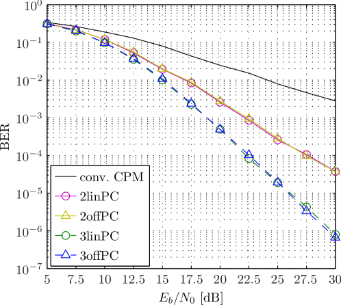
Figure 3: Simulated bit error rate (BER) over a Rayleigh fading channel

The received signal $y_{n}(t)$ is demodulated by the method introduced in Section III-A. The evaluated distances are fed to the Viterbi algorithm (VA), which we use for MLSE. The trellis decoded by the Viterbi algorithm has $pM^{\gamma-1}=16$ states and $L_{t}M=12$ paths leaving each state. In our simulations, the Viterbi algorithm is truncated to a path memory of 10 code blocks, which means that we get a decoding delay of $3\cdot 10T$.

Figure 3 shows the simulations results for one, two and three transmitting antennas. Both, linPC and offPC perform equally and corresponding to Section III-B it can be seen that full diversity is achieved. For high SNR the BER decreases with 5dB/dec and the three Tx antennas code achieves a decay of some 3.5dB/dec.

One of the main reason for using CPM for STC is their spectral efficiency. It should be noticed nevertheless that the introduction of a correction factor with non-zero mean in the phase signal induces a bandwidth expansion and thus degrades this spectral efficiency. However, as detailed in [17] the additional bandwidth requirements are quite moderate. Namely, to achieve an attenuation in power of -30dB for a linPC code with 3 Tx antennas, $h=1/2$, $g=2$ and $M=8$, a relative bandwidth expansion of only 7% is sufficient.

V Conclusion

In this paper, we introduce a new family of $L^{2}$-orthogonal STC for three antennas. These systems are based on CPM supplemented by correction factors to ensure $L^{2}$-orthogonality. Structurally the proposed code family has full rate and we provide the proof of full diversity. Furthermore, we detail two simple representatives of the code family (offPC, linPC), where the offPC offers better performance and a very intuitive representation. Finally, it should be noticed that our approach can easily be generalized to any number of transmitting antennas with full rate codes that also achieve full diversity.

References

- [1] I. E. Telatar, “Capacity of multi-antenna gaussian channels,” European Trans. Telecommun., vol. 10, pp. 585 – 595, 1999.
- [2] G. J. Foschini and M. J. Gans, “On limits of wireless communications in a fading environment when using multiple antennas,” Wirel. Pers. Commun., vol. 6, no. 3, pp. 311–335, 1998.
- [3] S. M. Alamouti, “A simple transmit diversity technique for wireless communications,” IEEE J. Sel. Areas Commun., vol. 16, no. 8, pp. 1451 – 1458, Oct. 1998.
- [4] V. Tarokh, H. Jafarkhani, and A. R. Calderbank, “Space–time block codes from orthogonal designs,” IEEE Trans. Inf. Theory, vol. 45, no. 5, pp. 1456 – 1567, July 1999.
- [5] V. Tarokh, N. Seshadri, and A. R. Calderbank, “Space-time codes for high data rate wireless communication: Performance criterion and code construction,” IEEE Trans. Inf. Theory, vol. 44, no. 2, pp. 744 – 765, march 1998.
- [6] X. Zhang and M. P. Fitz, “Space-time coding for Rayleigh fading channels in CPM system,” in Proc. of Annu. Allerton Conf. Communication, Control, and Computing, 2000.
- [7] ——, “Space-time code design with continuous phase modulation,” IEEE J. Sel. Areas Commun., vol. 21, pp. 783 – 792, June 2003.
- [8] A.-M. Silvester, L. Lampe, and R. Schober, “Diagonal space-time code design for continuous-phase modulation,” in Proc. of IEEE Global Telecommunications Conference (GLOBECOM ’06), Nov. 2006.
- [9] D. Bokolamulla and T. Aulin, “Serially concatenated space-time coded continuous phase modulated signals,” IEEE Trans. Wireless Commun., vol. 6, no. 10, pp. 3487 – 3492, 2007.
- [10] A. Zajić and G. Stüber, “A space-time code design for partial-response CPM: Diversity order and coding gain,” in Proc. of IEEE International Conference on Communications (ICC’07), June 2007, pp. 719 – 724.
- [11] G. Wang and X.-G. Xia, “An orthogonal space–time coded CPM system with fast decoding for two transmit antennas,” IEEE Trans. Inf. Theory, vol. 50, no. 3, pp. 486 – 493, March 2004.
- [12] D. Wang, G. Wang, and X.-G. Xia, “An orthogonal space–time coded partial response CPM system with fast decoding for two transmit antennas,” IEEE Trans. Wireless Commun., vol. 4, no. 5, pp. 2410 – 2422, Sept. 2005.
- [13] G. Wang, W. Su, and X.-G. Xia, “Orthogonal-like space-time coded CPM system with fast decoding for three and four transmit antennas,” in Proc. of IEEE Global Telecommunications Conference (GLOBECOM ’03), Nov. 2003, pp. 3321 – 3325.
- [14] M. Hesse, J. Lebrun, and L. Deneire, “L2 orthogonal space time code for continuous phase modulation,” in Proc. of IEEE Workshop on Signal Processing Advances in Wireless Communications (SPAWC’08), July 2008, pp. 401 – 405.
- [15] ——, “L2 OSTC-CPM: Theory and design,” CNRS/University of Nice, Sophia Antipolis, Tech. Rep. I3S/RR-2008-03, 2008. [Online]. Available: http://arxiv.org/abs/0806.2760
- [16] J. Anderson, T. Aulin, and C.-E. Sundberg, Digital Phase Modulation. Plenum Press, 1986.
- [17] M. Hesse, L. Deneire, and J. Lebrun, “Optimized L2-orthogonal STC CPM for 3 antennas,” in Proc. ISWCS’08, accepted for publication., Reykjavik, Iceland, 2008.
- [18] A. Zajić and G. Stüber, “Continuous phase modulated space-time codes,” in Proc. of IEEE International Symposium on Communication Theory and Applications (ISCTA’05), July 2005, pp. 292 – 297.