Development of the spectrum of gamma-ray burst pulses influenced by the intrinsic spectral evolution and the curvature effect

Abstract

Spectral evolution of gamma-ray burst pulses assumed to arise from emission of fireballs is explored. It is found that, due to the curvature effect, the integrated flux and peak energy are well related by a power law in the decaying phase of pulses, where the index is about 3, being free of the intrinsic emission and the Lorentz factor. The spectrum of a pulse in its decaying phase differs slightly for different intrinsic spectral evolution patterns, indicating that it is dominated by the curvature effect. In the rising phase, the integrated flux keeps increasing whilst the peak energy remains unchanged when the intrinsic emission bears an unchanged spectrum. Within this phase, the flux decreases with the increasing of the peak energy for a hard-to-soft intrinsic spectrum, and for a soft-to-hard-to-soft intrinsic spectrum, the flux generally increases with the increasing of the peak energy. An intrinsic soft-to-hard-to-soft spectral evolution within a co-moving pulse would give rise to a pulse-like evolutionary curve for the peak energy.

1 Introduction

Recent Swift observations of early X-ray afterglows of gamma-ray bursts (GRBs) revealed that the previous interpretation of the GRB afterglow, which is based on the mechanism of external shocks, is unlikely to be the mechanism accounting for these new findings. Instead, the internal shock origin and the so-called “curvature effect” might be responsible for many of the early X-ray afterglows [1-8]. The curvature effect is a combined effect that includes the delay of time and the shifting of the intrinsic spectrum as well as other relevant factors of an expanding fireball (see [9] for a detailed explanation). The effect was widely investigated in recent years in both the prompt emission and early X-ray afterglow of GRBs [4], [7-9], [10-23].

Early study of the spectral evolution of GRBs revealed that the general evolution of the spectra of these objects is hard-to-soft (e.g., [24]). This issue was also frequently investigated in recent years [11], [25-28]. Reference [14] showed that the hardness-intensity correlation could be accounted for by the curvature effect. Authors of [9] explored the evolutionary curve of the hardness ratio (HRC) of GRB pulses and concluded that the main characteristics of the HRC of some GRB FRED pulses are in agreement with what predicted by the curvature effect. In addition, they showed that the curvature effect alone could not completely explain the observed HRCs. Instead, a hard-to-soft intrinsic spectral evolution might exist and probably play a role in producing the observed HRCs.

Here, we investigate how the intrinsic spectral evolution and the curvature effect combine in producing an observed spectrum arising from a fireball pulse. The paper is organized as follows. In Section 2, we present formulas that can directly applied to the case of the intrinsic spectral evolution. Spectral evolution within a pulse of fireballs radiated with a typical intrinsic emission form is investigated in various aspects in Section 3. In Section 4, other intrinsic emission forms are considered. In Section 5, we pay our attention to various situations of the soft-to-hard-to-soft intrinsic emission. Influence of the Lorentz factor on the spectral evolution is investigated in Section 6. Presented in Section 7 is a signature of the curvature effect shown by the evolutionary curve of the peak energy in the decaying phase of pulses. Conclusions are given in Section 8.

2 General formulas of flux and count rates for expanding fireballs

Here we present more general formulas compared with those derived in [13] and [19] so that they could be directly applied to various cases of the intrinsic spectral evolution pattern. For more general applications, formulas with various variables are provided.

2.1 Formulas in terms of the integral of $\theta$

For a radiation associated with an intrinsic emission independent of direction, the expected flux of a fireball expanding with a constant Lorentz factor is [13]

$$f_{\nu}(t)=\frac{2\pi}{D^{2}}\int_{\widetilde{\theta}_{\min}}^{\widetilde{\theta}_{\max}}I_{\nu}(t^{\prime},\nu,\nu_{0})R^{2}(t^{\prime})\cos\theta\sin\theta d\theta,$$ (1)

where $I_{\nu}(t^{\prime},\nu,\nu_{0})$ is the observer frame intensity; $\nu$ is the observation frequency; $\nu_{0}$ is the rest frame frequency which emits from differential surface $ds_{\theta}$ and gives rise to $\nu$ (see equation 9 presented below for the relation between $I_{\nu}$ and $\nu_{0}$); $t$ is the observation time; $D$ is the distance of the fireball to the observer; $\theta$ is the angle, of $ds_{\theta}$, of the fireball, to the line of sight; $t^{\prime}$ is the emission time (in the observer frame), called local time, of photons which emit from $ds_{\theta}$; $R(t^{\prime})$ is the radius of the fireball measured at time $t^{\prime}$. The integral range of $\theta$, $\widetilde{\theta}_{\min}$ and $\widetilde{\theta}_{\max}$, will be determined by the concerned area of the fireball surface as well as the emission ranges of the frequency and the local time. As shown in [13] and [19], $t^{\prime}$ and $t$ are related by

$$t^{\prime}=\frac{t-t_{c}-\frac{D}{c}+\frac{R_{c}}{c}\cos\theta}{1-\beta\cos\theta}+t_{c},$$ (2)

where $t_{c}$ and $R_{c}$ are constants. Assume that the area of the fireball surface concerned is confined within

$$\theta_{\min}\leq\theta\leq\theta_{\max}$$ (3)

and the emission time $t^{\prime}$ is confined within

$$t_{c}\leq t_{\min}^{\prime}\leq t^{\prime}\leq t_{\max}^{\prime},$$ (4)

and besides them there are no other constraints to the integral limit of (1). According to (3) and (4), one can verify that the lower and upper integral limits of (1) could be determined by

$$\widetilde{\theta}_{\min}=\cos^{-1}\min\{\cos\theta_{\min},\frac{t_{\max}^{\prime}-t+\frac{D}{c}}{(t_{\max}^{\prime}-t_{c})\beta+\frac{R_{c}}{c}}\}$$ (5)

and

$$\widetilde{\theta}_{\max}=\cos^{-1}\max\{\cos\theta_{\max},\frac{t_{\min}^{\prime}-t+\frac{D}{c}}{(t_{\min}^{\prime}-t_{c})\beta+\frac{R_{c}}{c}}\},$$ (6)

respectively (for a detailed derivation, one could refer to [13] and [19]. Applying the relation between the radius of the fireball and the observation time we come to the following form of flux (see [13] and [19]):

$$f_{\nu}(t)=\frac{2\pi[(t-t_{c}-\frac{D}{c})\beta c+R_{c}]^{2}}{D^{2}}\int_{\widetilde{\theta}_{\min}}^{\widetilde{\theta}_{\max}}\frac{I_{\nu}(t^{\prime},\nu,\nu_{0})\cos\theta\sin\theta}{(1-\beta\cos\theta)^{2}}d\theta.$$ (7)

From (2) one finds that, for any given values of $t$ and $\theta$, local time $t^{\prime}$ would be uniquely determined. If this value of $t^{\prime}$ is within the range of (4), then there will be photons emitted at $t^{\prime}$ from the small surface area of $\theta$ reaching the observer at $t$ [when $\theta$ is within the range of (3), this small area would be included in the above integral, otherwise it would not]. Obviously, for a certain value of $\theta$, the range of $t$ depends on the range of $t^{\prime}$. Inserting (2) into (4) and applying (3) we obtain

$$\begin{array}[]{l}(1-\beta\cos\theta_{\min})t_{\min}^{\prime}+(t_{c}\beta-\frac{R_{c}}{c})\cos\theta_{\min}+\frac{D}{c}\leq t\\ \leq(1-\beta\cos\theta_{\max})t_{\max}^{\prime}+(t_{c}\beta-\frac{R_{c}}{c})\cos\theta_{\max}+\frac{D}{c}\end{array}.$$ (8)

It suggests clearly that observation time $t$ is limited when emission time $t^{\prime}$ is limited.

Let $t_{0}$ be the proper time corresponding to the coordinate time $t^{\prime}$ and $\nu_{0}$ be the co-moving frequency corresponding to $\nu$. The latter two are related by the Doppler effect. It is well known that the observer frame intensity $I_{\nu}(t^{\prime},\nu,\nu_{0})$ is related to the rest frame intensity $I_{0,\nu}(t_{0},\nu_{0})$ by

$$I_{\nu}(t^{\prime},\nu,\nu_{0})=(\frac{\nu}{\nu_{0}})^{3}I_{0,\nu}(t_{0},\nu_{0}),$$ (9)

which could be written by

$$I_{\nu}(t^{\prime},\nu,\nu_{0})=\frac{I_{0,\nu}(t_{0},\nu_{0})}{(1-\beta\cos\theta)^{3}\Gamma^{3}}$$ (10)

when applying the Doppler effect. The flux is now able to be written by

$$f_{\nu}(t)=\frac{2\pi[(t-t_{c}-\frac{D}{c})\beta c+R_{c}]^{2}}{D^{2}\Gamma^{3}}\int_{\widetilde{\theta}_{\min}}^{\widetilde{\theta}_{\max}}\frac{I_{0,\nu}(t_{0},\nu_{0})\cos\theta\sin\theta}{(1-\beta\cos\theta)^{5}}d\theta,$$ (11)

where $\widetilde{\theta}_{\min}$ and $\widetilde{\theta}_{\max}$ are determined by (5) and (6), respectively, $\nu_{0}$ and $\nu$ are related by the Doppler effect, and $t$ is confined by (8).

As $t_{0}$ and $t^{\prime}$ represent the same moment, according to the theory of special relativity, they are related by $t^{\prime}-t_{c}=\Gamma(t_{0}-t_{0,c})$, where $t_{0,c}$ is a constant (here we assign $t^{\prime}=t_{c}$ when $t_{0}=t_{0,c}$). Assign $t^{\prime}=t_{\min}^{\prime}|_{t_{0}=t_{0,\min}}$ and $t^{\prime}=t_{\max}^{\prime}|_{t_{0}=t_{0,\max}}$. We get $t_{\min}^{\prime}=\Gamma(t_{0,\min}-t_{0,c})+t_{c}$, and $t_{\max}^{\prime}=\Gamma(t_{0,\max}-t_{0,c})+t_{c}$. Then the constraint of (4) is identical to

$$t_{0,c}\leq t_{0,\min}\leq t_{0}\leq t_{0,\max}.$$ (12)

We then get from (5)-(6) that

$$\widetilde{\theta}_{\min}=\cos^{-1}\min\{\cos\theta_{\min},\frac{(t_{0,\max}-t_{0,c})\Gamma+\frac{D}{c}-(t-t_{c})}{(t_{0,\max}-t_{0,c})\Gamma\beta+\frac{R_{c}}{c}}\}$$ (13)

and

$$\widetilde{\theta}_{\max}=\cos^{-1}\max\{\cos\theta_{\max},\frac{(t_{0,\min}-t_{0,c})\Gamma+\frac{D}{c}-(t-t_{c})}{(t_{0,\min}-t_{0,c})\Gamma\beta+\frac{R_{c}}{c}}\}.$$ (14)

In addition, from (2) and $t^{\prime}-t_{c}=\Gamma(t_{0}-t_{0,c})$ we obtain

$$t_{0}=\frac{t-t_{c}-\frac{D}{c}+\frac{R_{c}}{c}\cos\theta}{(1-\beta\cos\theta)\Gamma}+t_{0,c}$$ (15)

and from $t_{\min}^{\prime}=\Gamma(t_{0,\min}-t_{0,c})+t_{c}$, $t_{\max}^{\prime}=\Gamma(t_{0,\max}-t_{0,c})+t_{c}$, and (8) we gain

$$\begin{array}[]{l}(1-\beta\cos\theta_{\min})[(t_{0,\min}-t_{0,c})\Gamma+t_{c}]+(t_{c}\beta-\frac{R_{c}}{c})\cos\theta_{\min}+\frac{D}{c}\leq t\\ \leq(1-\beta\cos\theta_{\max})[(t_{0,\max}-t_{0,c})\Gamma+t_{c}]+(t_{c}\beta-\frac{R_{c}}{c})\cos\theta_{\max}+\frac{D}{c}\end{array}.$$ (16)

When calculating the flux from (11), we need to convert variable $t_{0}$ to $\theta$ via (15) and convert $\nu_{0}$ to $\theta$ according to the Doppler effect $\nu_{0}=(1-\beta\cos\theta)\Gamma\nu$.

Light curves of gamma-ray bursts are always presented in terms of count rates within an energy range. The count rate within energy channel $[\nu_{1},\nu_{2}]$ is determined by

$$\frac{dn(t)}{dt}=\int_{\nu_{1}}^{\nu_{2}}\frac{f_{\nu}(t)}{h\nu}d\nu.$$ (17)

Inserting (11) leads to

$$\frac{dn(t)}{dt}=\frac{2\pi[(t-t_{c}-\frac{D}{c})\beta c+R_{c}]^{2}}{D^{2}\Gamma^{3}h}\int_{\widetilde{\theta}_{\min}}^{\widetilde{\theta}_{\max}}[\int_{\nu_{1}}^{\nu_{2}}\frac{I_{0,\nu}(t_{0},\nu_{0})}{\nu}d\nu]\frac{\cos\theta\sin\theta}{(1-\beta\cos\theta)^{5}}d\theta.$$ (18)

In the case that $\theta$ could be treated as a constant, from $\nu_{0}=(1-\beta\cos\theta)\Gamma\nu$ one gets $\frac{d\nu}{\nu}|_{\theta=const}=\frac{d\nu_{0}}{\nu_{0}}$. Replacing variable $\nu$ with $\nu_{0}$ we get from (18) that

$$\frac{dn(t)}{dt}=\frac{2\pi[(t-t_{c}-\frac{D}{c})\beta c+R_{c}]^{2}}{D^{2}\Gamma^{3}h}\int_{\widetilde{\theta}_{\min}}^{\widetilde{\theta}_{\max}}[\int_{\nu_{0,1}}^{\nu_{0,2}}\frac{I_{0,\nu}(t_{0},\nu_{0})}{\nu_{0}}d\nu_{0}]\frac{\cos\theta\sin\theta}{(1-\beta\cos\theta)^{5}}d\theta$$ (19)

where $\nu_{0,1}=(1-\beta\cos\theta)\Gamma\nu_{1}$ and $\nu_{0,2}=(1-\beta\cos\theta)\Gamma\nu_{2}$.

2.2 Formulas in terms of the integral of $\cos\theta$

In terms of the integral of $\cos\theta$, the forms of the above formulas become simpler. Let

$$\mu\equiv\cos\theta,$$ (20)

$$\mu_{\max}\equiv\cos\widetilde{\theta}_{\min}=\min\{\cos\theta_{\min},\frac{(t_{0,\max}-t_{0,c})\Gamma+\frac{D}{c}-(t-t_{c})}{(t_{0,\max}-t_{0,c})\Gamma\beta+\frac{R_{c}}{c}}\}$$ (21)

and

$$\mu_{\min}\equiv\cos\widetilde{\theta}_{\max}=\max\{\cos\theta_{\max},\frac{(t_{0,\min}-t_{0,c})\Gamma+\frac{D}{c}-(t-t_{c})}{(t_{0,\min}-t_{0,c})\Gamma\beta+\frac{R_{c}}{c}}\},$$ (22)

where (13)-(14) are applied.

The flux now can be calculated by

$$f_{\nu}(t)=\frac{2\pi[(t-t_{c}-\frac{D}{c})\beta c+R_{c}]^{2}}{D^{2}\Gamma^{3}}\int_{\mu_{\min}}^{\mu_{\max}}\frac{I_{0,\nu}(t_{0},\nu_{0})\mu}{(1-\beta\mu)^{5}}d\mu,$$ (23)

where $t_{0}$ and $\mu$ are related by

$$t_{0}=\frac{t-t_{c}-\frac{D}{c}+\frac{R_{c}}{c}\mu}{(1-\beta\mu)\Gamma}+t_{0,c}$$ (24)

and $\nu_{0}$ and $\mu$ are related by $\nu_{0}=(1-\beta\mu)\Gamma\nu$.

The count rate is now determined by

$$\frac{dn(t)}{dt}=\frac{2\pi[(t-t_{c}-\frac{D}{c})\beta c+R_{c}]^{2}}{D^{2}\Gamma^{3}h}\int_{\mu_{\min}}^{\mu_{\max}}[\int_{\nu_{0,1}}^{\nu_{0,2}}\frac{I_{0,\nu}(t_{0},\nu_{0})}{\nu_{0}}d\nu_{0}]\frac{\mu}{(1-\beta\mu)^{5}}d\mu,$$ (25)

where $\nu_{0,1}=(1-\beta\mu)\Gamma\nu_{1}$ and $\nu_{0,2}=(1-\beta\mu)\Gamma\nu_{2}$.

2.3 Formulas in terms of the integral of the proper emission time

Since the rest frame intensity $I_{0,\nu}(t_{0},\nu_{0})$ is always provided in the form of the function of the proper emission time $t_{0}$, it would be more convenient to compute the flux or the count rate with formulas in terms of the integral of $t_{0}$.

From (24) we get

$$\mu=\frac{(t_{0}-t_{0,c})\Gamma+\frac{D}{c}-(t-t_{c})}{\frac{R_{c}}{c}+(t_{0}-t_{0,c})\Gamma\beta},$$ (26)

and from $\nu_{0}=(1-\beta\mu)\Gamma\nu$ we find

$$\nu_{0}=\frac{\frac{R_{c}}{c}-[\frac{D}{c}-(t-t_{c})]\beta}{\frac{R_{c}}{c}+(t_{0}-t_{0,c})\Gamma\beta}\Gamma\nu.$$ (27)

According to (26) and (27) one can check that $\frac{dt_{0}}{d\mu}>0$.

Replacing $\mu$ with $t_{0}$, we obtain the following form of formula for calculating the flux

$$f_{\nu}(t)=\frac{2\pi c^{2}\int_{\widetilde{t}_{0,\min}}^{\widetilde{t}_{0,\max}}I_{0,\nu}(t_{0},\nu_{0})[(t_{0}-t_{0,c})\Gamma+\frac{D}{c}-(t-t_{c})][\frac{R_{c}}{c}+(t_{0}-t_{0,c})\Gamma\beta]^{2}dt_{0}}{D^{2}\Gamma^{2}\{\frac{R_{c}}{c}-[\frac{D}{c}-(t-t_{c})]\beta\}^{2}},$$ (28)

where $\widetilde{t}_{0,\min}$ and $\widetilde{t}_{0,\max}$ are determined by

$$\widetilde{t}_{0,\min}=\max\{t_{0,\min},\frac{t-t_{c}-\frac{D}{c}+\frac{R_{c}}{c}\cos\theta_{\max}}{(1-\beta\cos\theta_{\max})\Gamma}+t_{0,c}\}$$ (29)

and

$$\widetilde{t}_{0,\max}=\min\{t_{0,\max},\frac{t-t_{c}-\frac{D}{c}+\frac{R_{c}}{c}\cos\theta_{\min}}{(1-\beta\cos\theta_{\min})\Gamma}+t_{0,c}\},$$ (30)

respectively, and $\nu_{0}$ and $t_{0}$ are related by (27).

The count rate is now written in the form

$$\frac{dn(t)}{dt}=\frac{2\pi c^{2}\int_{\widetilde{t}_{0,\min}}^{\widetilde{t}_{0,\max}}[\int_{\nu_{1}}^{\nu_{2}}I_{0,\nu}(t_{0},\nu_{0})\frac{d\nu}{\nu}][(t_{0}-t_{0,c})\Gamma+\frac{D}{c}-(t-t_{c})][\frac{R_{c}}{c}+(t_{0}-t_{0,c})\Gamma\beta]^{2}dt_{0}}{D^{2}\Gamma^{2}h\{\frac{R_{c}}{c}-[\frac{D}{c}-(t-t_{c})]\beta\}^{2}}.$$ (31)

According to (27), in the case that $t$ and $t_{0}$ could be treated as constants we get $\frac{d\nu}{\nu}|_{t_{0}=const,t=const}=\frac{d\nu_{0}}{\nu_{0}}$. Replacing variable $\nu$ with $\nu_{0}$ we get from (31) that

$$\frac{dn(t)}{dt}=\frac{2\pi c^{2}\int_{\widetilde{t}_{0,\min}}^{\widetilde{t}_{0,\max}}[\int_{\nu_{0,1}}^{\nu_{0,2}}\frac{I_{0,\nu}(t_{0},\nu_{0})}{\nu_{0}}d\nu_{0}][(t_{0}-t_{0,c})\Gamma+\frac{D}{c}-(t-t_{c})][\frac{R_{c}}{c}+(t_{0}-t_{0,c})\Gamma\beta]^{2}dt_{0}}{D^{2}\Gamma^{2}h\{\frac{R_{c}}{c}-[\frac{D}{c}-(t-t_{c})]\beta\}^{2}},$$ (32)

where $\nu_{0,1}=[\frac{R_{c}}{c}-(\frac{D}{c}-t+t_{c})\beta]\Gamma\nu_{1}/[\frac{R_{c}}{c}+(t_{0}-t_{0,c})\Gamma\beta]$ and $\nu_{0,2}=[\frac{R_{c}}{c}-(\frac{D}{c}-t+t_{c})\beta]\Gamma\nu_{2}/[\frac{R_{c}}{c}+(t_{0}-t_{0,c})\Gamma\beta]$.

2.4 Formulas in terms of the integral of relative timescales

Assign [19]

$$\tau^{\prime}\equiv\frac{t^{\prime}-t_{c}}{\frac{R_{c}}{c}},\qquad\tau_{\min}^{\prime}\equiv\frac{t_{\min}^{\prime}-t_{c}}{\frac{R_{c}}{c}},\qquad\tau_{\max}^{\prime}\equiv\frac{t_{\max}^{\prime}-t_{c}}{\frac{R_{c}}{c}},$$ (33)

$$\tau_{0}\equiv\frac{t_{0}-t_{0,c}}{\frac{R_{c}}{c}},\qquad\tau_{0,\min}\equiv\frac{t_{0,\min}-t_{0,c}}{\frac{R_{c}}{c}},\qquad\tau_{0,\max}\equiv\frac{t_{0,\max}-t_{0,c}}{\frac{R_{c}}{c}},$$ (34)

and

$$\tau\equiv\frac{t-t_{c}-\frac{D}{c}+\frac{R_{c}}{c}}{\frac{R_{c}}{c}}.$$ (35)

One finds that

$$\nu_{0}=\frac{1-\beta+\beta\tau}{1+\beta\Gamma\tau_{0}}\Gamma\nu,$$ (36)

$$\tau^{\prime}=\frac{\tau-(1-\cos\theta)}{1-\beta\cos\theta},$$ (37)

$$0\leq\tau_{\min}^{\prime}\leq\tau^{\prime}\leq\tau_{\max}^{\prime},$$ (38)

and

$$1-\cos\theta_{\min}+(1-\beta\cos\theta_{\min})\tau_{\min}^{\prime}\leq\tau\leq 1-\cos\theta_{\max}+(1-\beta\cos\theta_{\max})\tau_{\max}^{\prime}$$ (39)

[which is the range of $\tau$ within which the radiation defined within (3) and (4) is observable]. In addition, one gets $\tau_{0,\min}=\frac{\tau_{\min}^{\prime}}{\Gamma}$, $\tau_{0,\max}=\frac{\tau_{\max}^{\prime}}{\Gamma}$, and

$$1-\cos\theta_{\min}+(1-\beta\cos\theta_{\min})\Gamma\tau_{0,\min}\leq\tau\leq 1-\cos\theta_{\max}+(1-\beta\cos\theta_{\max})\Gamma\tau_{0,\max}.$$ (40)

Let

$$\widetilde{I}_{0,\nu}(\tau_{0},\nu_{0})\equiv I_{0,\nu}[t_{0}(\tau_{0}),\nu_{0}].$$ (41)

We get from (28) that

$$f_{\nu}(\tau)=\frac{2\pi R_{c}^{2}\int_{\widetilde{\tau}_{0,\min}}^{\widetilde{\tau}_{0,\max}}\widetilde{I}_{0,\nu}(\tau_{0},\nu_{0})(1-\tau+\tau_{0}\Gamma)(1+\Gamma\beta\tau_{0})^{2}d\tau_{0}}{D^{2}\Gamma^{2}(1-\beta+\beta\tau)^{2}},$$ (42)

where $\nu_{0}$ is related to $\tau$ and $\nu$ by (36),

$$\widetilde{\tau}_{0,\min}=\frac{\widetilde{t}_{0,\min}-t_{0,c}}{\frac{R_{c}}{c}}=\max\{\tau_{0,\min},\frac{\tau-1+\cos\theta_{\max}}{(1-\beta\cos\theta_{\max})\Gamma}\},$$ (43)

and

$$\widetilde{\tau}_{0,\max}=\frac{\widetilde{t}_{0,\max}-t_{0,c}}{\frac{R_{c}}{c}}=\min\{\tau_{0,\max},\frac{\tau-1+\cos\theta_{\min}}{(1-\beta\cos\theta_{\min})\Gamma}\}.$$ (44)

Let

$$C(\tau)\equiv\frac{dn[t(\tau)]}{d\tau}.$$ (45)

We then get

$$C(\tau)=\frac{2\pi R_{c}^{3}\int_{\widetilde{\tau}_{0,\min}}^{\widetilde{\tau}_{0,\max}}[\int_{\nu_{0,1}}^{\nu_{0,2}}\frac{\widetilde{I}_{0,\nu}(\tau_{0},\nu_{0})}{\nu_{0}}d\nu_{0}](1-\tau+\Gamma\tau_{0})(1+\beta\Gamma\tau_{0})^{2}d\tau_{0}}{hcD^{2}\Gamma^{2}(1-\beta+\beta\tau)^{2}}.$$ (46)

where $\nu_{0,1}=\frac{(1-\beta+\beta\tau)\Gamma}{1+\beta\Gamma\tau_{0}}\nu_{1}$ and $\nu_{0,2}=\frac{(1-\beta+\beta\tau)\Gamma}{1+\beta\Gamma\tau_{0}}\nu_{2}$. Note that (42) and (46) hold only when (40) is satisfied. In the range beyond (40), $f_{\nu}(\tau)$ and $C(\tau)$ will become zero.

Formula (46) shows that the profile of count rates of a fireball source is a function of $\tau$. It is independent of the real time scale $t$, and independent of the real size, $R_{c}$, of the source. In other words, no matter how large is the fireball concerned and how large is the observed timescale concerned, for the profile of the count rate, only the ratio of the latter to the time scale of the initial radius of the fireball plays a role.

Applying (33) and (34) to $t^{\prime}-t_{c}=\Gamma(t_{0}-t_{0,c})$ we get $\tau^{\prime}=\Gamma\tau_{0}$. Substituting it into (37) comes to

$$\tau_{0}=\frac{\tau-(1-\cos\theta)}{(1-\beta\cos\theta)\Gamma}.$$ (47)

Generally, observation time $\tau$ is related to the co-moving time $\tau_{0}$ of the surface with $\theta$ by

$$\tau=(1-\beta\cos\theta)\Gamma\tau_{0}+1-\cos\theta.$$ (48)

For the same emission time $\tau_{0}$, photons emitted from surfaces with different line-of-sight angles would reach the observer at different times. In units of the time scale of the initial radius $R_{c}$, the time delay of photons emitted from $\theta$ relative to that of those emitted from $\theta=0$ is $1-\cos\theta$. The contraction factor of the emission time is $(1-\beta\cos\theta)\Gamma$ which differs from surface to surface. Taking $\theta=0$ we gain

$$\tau=(1-\beta)\Gamma\tau_{0}\qquad\qquad(\theta=0).$$ (49)

This is the relation that relates the observation time of photons which are emitted from $\theta=0$ with the corresponding co-moving emission time. The time is contracted by a factor of $(1-\beta)\Gamma$.

3 Spectral evolution within the period of fireball pulses coming from a typical intrinsic emission form

As revealed in [9], the observed hardness ratio is seen to be harder at the beginning of some GRB pulses than what the pure curvature effect (when no intrinsic spectral evolution is involved) could predict and be softer at later times of the pulses, causing a so-called “harder-leading” problem. An economic mechanism was suggested to account for this problem, which is the hard-to-soft evolution pattern of the rest frame spectrum of fireballs (see [9]). In a more realistic situation, before the hardest spectrum appears, there might be a short period within which the co-moving spectrum undergoes a soft-to-hard phase. This would happen when the inner shell possesses a relatively harder core and surrounding the core are attached with less dense materials. The hardest spectrum will appear when the core strikes the outer shell. Before that the spectrum radiated from the outer shell is softer since the shell is hit by relatively less dense materials and then gains a much smaller acceleration and a smaller speed.

Let us investigate the spectral evolution in a simple case where the emission of a co-moving pulse with an exponential rise and exponential decay and with a flexible Comptonized radiation form from the whole fireball surface is observed. For the sake of comparison, we consider three co-moving pulses (or rest frame pulses) with their spectra being unchanged, hard-to-soft, and soft-to-hard-to-soft respectively during the period concerned. The co-moving pulse with an unchanged spectrum is assumed to be

$$\widetilde{I}_{0,\nu}(\tau_{0},\nu_{0})=I_{0}\nu_{0}^{1+\alpha_{C}}\exp(-\nu_{0}/\nu_{0,C})\{\begin{array}[]{c}\exp(-\frac{\tau_{0,0}-\tau_{0}}{\sigma_{r}})\qquad(\tau_{0,\min}\leq\tau_{0}\leq\tau_{0,0})\\ \exp(-\frac{\tau_{0}-\tau_{0,0}}{\sigma_{d}})\qquad\qquad\qquad(\tau_{0,0}<\tau_{0})\end{array}.$$ (50)

The co-moving pulse (50) is intrinsically the same as that adopted in [9]. [Note that, $\tau^{\prime}=\Gamma\tau_{0}$, or $\tau_{0}\propto\tau^{\prime}$.] The co-moving pulse possessing a hard-to-soft spectral evolution is assumed to be

$$\widetilde{I}_{0,\nu}(\tau_{0},\nu_{0})=I_{0}\nu_{0}^{1+\alpha_{C}}\exp[-(\tau_{0}/\tau_{0,0})(\nu_{0}/\nu_{0,C})]\{\begin{array}[]{c}\exp(-\frac{\tau_{0,0}-\tau_{0}}{\sigma_{r}})\qquad(\tau_{0,\min}\leq\tau_{0}\leq\tau_{0,0})\\ \exp(-\frac{\tau_{0}-\tau_{0,0}}{\sigma_{d}})\qquad\qquad\qquad(\tau_{0,0}<\tau_{0})\end{array},$$ (51)

where $\tau_{0,0}\neq 0$. The co-moving pulse with a soft-to-hard-to-soft spectrum is assumed to be

$$\widetilde{I}_{0,\nu}(\tau_{0},\nu_{0})=I_{0}\nu_{0}^{1+\alpha_{C}}\{\begin{array}[]{c}\exp[-(\tau_{0,0}/\tau_{0})(\nu_{0}/\nu_{0,C})]\exp(-\frac{\tau_{0,0}-\tau_{0}}{\sigma_{r}})\qquad(\tau_{0,\min}<\tau_{0}\leq\tau_{0,0})\\ \exp[-(\tau_{0}/\tau_{0,0})(\nu_{0}/\nu_{0,C})]\exp(-\frac{\tau_{0}-\tau_{0,0}}{\sigma_{d}})\qquad\qquad\qquad(\tau_{0,0}<\tau_{0})\end{array},$$ (52)

where $\tau_{0}>0$ is required (as shown below, this will easily be satisfied). As adopted previously, we assign $\tau_{0}=10\sigma_{r}+\tau_{0,\min}$. According to (4), we assign $t^{\prime}\geq t_{c}$, which leads to $\tau_{0,\min}\geq 0$. As long as this condition is satisfied, $\tau_{0,\min}$ could be freely chosen. [Note that, in the case that $t^{\prime}\geq t_{c}$ does not hold, $\tau_{0,\min}$ is also constrained: $\tau_{0,\min}>-(\beta\Gamma)^{-1}$, when $\beta>0$ (see [19]). Without any loss of generality we take $\tau_{0,\min}=0$. To meet the condition that the soft-to-hard period is much shorter than the hard-to-soft phase in the third co-moving pulse, we take $\sigma_{d}=2\sigma_{r}$ and this will be applied to all the three co-moving pulses in the following analysis.

Figure 1: Spectral evolutions of co-moving pulses (50) (the lower panel), (51) (the mid panel), and (52) (the upper panel), where we take $\sigma_{r}=0.01$, $\sigma_{d}=2\sigma_{r}$, $\alpha_{0,C}=-0.6$, $\nu_{0,C}=1keVh^{-1}$, and $I_{0}=1$. Solid lines from the bottom to the top stand for the co-moving times $\tau_{0}(1)$, $\tau_{0}(2)$, and $\tau_{0}(3)$, respectively, and dashed lines from the top to the bottom represent $\tau_{0}(4)$, $\tau_{0}(5)$, $\tau_{0}(6)$, $\tau_{0}(7)$, $\tau_{0}(8)$, $\tau_{0}(9)$ , and $\tau_{0}(10)$, respectively.

Shown in Fig. 1 are the spectral evolutions of the three co-moving pulses (50), (51), and (52), where the co-moving times concerned are $\tau_{0}(1)=\tau_{0,0}-2\sigma_{r}$, $\tau_{0}(2)=\tau_{0,0}-\sigma_{r}$, $\tau_{0}(3)=\tau_{0,0}$, $\tau_{0}(4)=\tau_{0,0}+\sigma_{d}$, $\tau_{0}(5)=\tau_{0,0}+2\sigma_{d}$, $\tau_{0}(6)=\tau_{0,0}+4\sigma_{d}$, $\tau_{0}(7)=\tau_{0,0}+6\sigma_{d}$, $\tau_{0}(8)=\tau_{0,0}+8\sigma_{d}$, $\tau_{0}(9)=\tau_{0,0}+10\sigma_{d}$, and $\tau_{0}(10)=\tau_{0,0}+12\sigma_{d}$, respectively.

Figure 2: Positions of the observation times corresponding to various co-moving times for photons emitted from the tip of the fireball ($\theta=0$) marked in the light curves expected by distant observers. The light curves associated with co-moving pulses (50) (lower panels), (51) (mid panels), and (52) (upper panels) are calculated with equation (46), where we take $\sigma_{d}=2\sigma_{r}$, $\alpha_{0,C}=-0.6$, $\nu_{0,C}=1keVh^{-1}$, $\Gamma=100$, and $C_{0}\equiv 2\pi R_{c}^{3}I_{0}/hcD^{2}=1$. The width in the rising part of the co-moving pulses is taken as $\sigma_{r}=0.0001$ (left panels) and $\sigma_{r}=0.01$ (right panels), which correspond to “narrow” and “broad” pulses, respectively (see [17] and [19]). Solid lines stand for the light curves expected in the third channel of BATSE ($55keV\leq E<110keV$). Dashed lines from the left to the right represent observation times $\tau(1)$, $\tau(2)$, $\tau(3)$, $\tau(4)$, $\tau(5)$, $\tau(6)$, $\tau(7)$, $\tau(8)$, $\tau(9)$, and $\tau(10)$, respectively.

Let us check how these co-moving pulses give rise to the spectra of fireballs. According to (49), the observation times of photons which are emitted from the tip of the fireball (i.e., $\theta=0$) at the above co-moving times are $\tau(1)=(1-\beta)\Gamma(\tau_{0,0}-2\sigma_{r})$, $\tau(2)=(1-\beta)\Gamma(\tau_{0,0}-\sigma_{r})$, $\tau(3)=(1-\beta)\Gamma(\tau_{0,0})$, $\tau(4)=(1-\beta)\Gamma(\tau_{0,0}+\sigma_{d})$, $\tau(5)=(1-\beta)\Gamma(\tau_{0,0}+2\sigma_{d})$, $\tau(6)=(1-\beta)\Gamma(\tau_{0,0}+4\sigma_{d})$, $\tau(7)=(1-\beta)\Gamma(\tau_{0,0}+6\sigma_{d})$, $\tau(8)=(1-\beta)\Gamma(\tau_{0,0}+8\sigma_{d})$, $\tau(9)=(1-\beta)\Gamma(\tau_{0,0}+10\sigma_{d})$, and $\tau(10)=(1-\beta)\Gamma(\tau_{0,0}+12\sigma_{d})$, respectively. Positions of these times in the light curves observed by distant observers are shown in Fig. 2, where, (46) is employed to calculate the corresponding light curves. Note that, equation (21) in [19] could only be applied to a simple case when the time component and the spectral component of an intrinsic pulse could be separated (see equation (10) in [19]). The advantage of equation (46) is that it could be directly applied to a co-moving radiation which can take any forms. For the same reason, (42) will be applied to calculate the observed spectrum in the following analysis.

In Fig. 2, two typical widthes of co-moving pulses are adopted to show how the co-moving width influences the observed spectrum. They are $\sigma_{r}=0.0001$ and $\sigma_{r}=0.01$ in co-moving pulses (50)-(52), which correspond to relatively narrow and broad pulses respectively (see [17] and [19]). The words “narrow” and “broad” refer to the profile of the observed pulses. A “narrow” pulse comes from a local pulse with a small ratio of its width to the radius of the fireball [or, the ratio of the co-moving pulse width to the product of the radius of the fireball and the Lorentz factor is small; see equation (49)]. A character of this kind of pulse is that the pulse possesses a more steadily decaying phase. Or more precisely, the deviation of its decaying profile to the so-called standard decaying form is mild (for a detailed explanation, see [17]). Conversely, a “broad” pulse arises from a local pulse with a large ratio of its width to the radius of the fireball. A character of this kind of pulse is that its decaying profile possesses a reverse S-feature deviation from the standard decaying curve (or the deviation is very obvious) [17].

3.1 Evolutionary pattern of the overall spectrum

Displayed in Fig. 3 are the spectral evolutions within the period of the expected observed pulses of fireballs, which are outcomes of the three co-moving pulses (50), (51), and (52). We use equation (42) to calculate the spectra measured at the observation times $\tau(1)$, $\tau(2)$, $\tau(3)$, $\tau(4)$, $\tau(5)$, $\tau(6)$, $\tau(7)$, $\tau(8)$, $\tau(9)$, and $\tau(10)$. The resulted overall spectra show a general hard-to-soft evolution pattern within the period of the pulses observed. During these observation times, the spectral evolution of “narrow” pulses is mild (see Fig. 3 left panels), while for “broad” pulses their spectra develop quite rapidly (see Fig. 3 right panels). In the decaying part of light curves of “narrow” or “broad” pulses, the spectral evolution patterns are quite similar for the three co-moving pulses (see dashed lines in Fig. 3). This must be due to the fact that the decaying part of the pulses is dominated by high latitude emission of the fireball, where the curvature effect is important. It is then natural that the spectral evolutions show a similar trend. In the rising part of the light curves of pulses, the situation is different. The spectral evolution pattern of co-moving pulses obviously influences the way the observed spectrum evolves.

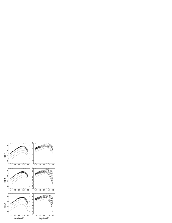
Figure 3: Spectral evolutions of fireball pulses arising from co-moving pulses (50) (lower panels), (51) (mid panels), and (52) (upper panels). The spectra are calculated with (42). Each panel in this plot corresponds to the same panel in Fig. 2, where the parameters are the same. The only difference is that we take $F_{0}\equiv 2\pi R_{c}^{2}I_{0}/D^{2}=1$. In the left panels, solid lines from the bottom to the top stand for the spectra measured at observation times $\tau(1)$, $\tau(2)$, $\tau(3)$, $\tau(4)$, and $\tau(5)$, respectively, while dashed lines from the top to the bottom represent the spectra measured at $\tau(6)$, $\tau(7)$, $\tau(8)$, $\tau(9)$, and $\tau(10)$, respectively. In the right panels, solid lines from the bottom to the top stand for the spectra measured at $\tau(1)$, $\tau(2)$, $\tau(3)$, and $\tau(4)$, respectively, and dashed lines from the top to the bottom denote the spectra measured at $\tau(5)$, $\tau(6)$, $\tau(7)$, $\tau(8)$, $\tau(9)$, and $\tau(10)$, respectively.

3.2 Evolution of the peak energy of the $\nu f_{\nu}$ spectrum

There are two quantities capable of describing the hardness of spectra. One is the so-called hardness ratio and the other is the peak energy $E_{p}$, the energy where the peak of $\nu f_{\nu}$ is observed. Evolutions of the two quantities could describe in some extent how the spectrum evolves. Recently, the hardness ratio curves associated with different situations were discussed [9]. Here, we pay our attention mainly to the evolution of the peak energy within the period of fireball pulses which arise from the three co-moving pulses proposed above.

We employ the following integrated flux (see Section 5) to compare the evolution of $E_{p}$ with light curves:

$$F\equiv\int_{\nu_{1}}^{\nu_{2}}f_{\nu}d\nu$$ (53)

where $\nu_{1}$ and $\nu_{2}$ are the lower and upper limits of the energy channel concerned.

Figure 4: Evolutionary curves of the peak energy (upper panels) of fireball pulses arising from co-moving pulses (50) (dotted lines), (51) (solid lines), and (52) (dashed lines). For the sake of comparison, we present in the lower panels the integrated flux $F_{2+3}$ over the the energy range of the second ($55keV\leq E<110keV$) and third ($110keV\leq E<320keV$) BATSE channels, which are calculated with (42) and (53). Parameters are the same as they are in Fig. 2. As adopted in Fig. 2, the width in the rising part of the co-moving pulses is taken as $\sigma_{r}=0.0001$ (left panels) and $\sigma_{r}=0.01$ (right panels), which correspond to “narrow” and “broad” pulses, respectively.

Displayed in Fig. 4 are the developments of the peak energy in various cases considered above. We find that the feature of drop-to-rise-to-drop revealed in the hardness ratio curve in [9] is observed in the peak energy evolutionary curve and it holds only for the unchanged intrinsic spectrum. In the case of intrinsically hard-to-soft spectrum, we observe a continuous hard-to-soft pattern, while in the case of intrinsically soft-to-hard-to-soft spectrum, one finds a soft-to-hard-to-soft evolution pattern for the observed spectrum. There is a turning point in the $E_{p}(t)$ curve (hereafter EPC). After the turning point, the EPCs associated with the three co-moving pulses show the same trend of softening in the case of “narrow” pulses. Before the turning point, the observed spectra vary significantly in accordant with their intrinsic spectral evolution patterns. This suggests that the spectrum observed before the turning point must mainly be determined by the intrinsic evolution pattern, while after the turning point, it is dominated by the curvature effect. In the “broad” pulse cases, the softening of the spectra arising from the un-changed intrinsic spectrum co-moving pulses are different from that of the hard-to-soft and soft-to-hard-to-soft intrinsic spectrum co-moving pulses, which leads to a noticeable character discussed below. The sharpness of the turning feature might become an indicator showing a pulse observed is “narrow” or “broad”.

3.3 Comparison of the spectrum of the emission of the tip with that arising from the overall fireball surface

If the fireball moves relativistically towards the observer but not expands, one would observed an entirely different evolution pattern of the spectrum within the pulse concerned. Compared with this spectrum, is that arising from the expanding fireball harder or softer? An investigation on this issue might bring us some interesting information. The spectrum of an ejecta moving towards the observer must be the same as that emitted from the tip of an expanding fireball surface when the intrinsic spectra and the Lorentz factors are the same.

The spectrum of the emission from the tip of the fireball surface must merely be a blue-shifting of the intrinsic one. Due to the contribution of high latitude emissions, a deviation of the observed spectrum of the whole fireball from that of the tip is expected. If the deviation is small within some period of observation time, then one can estimates the form of the intrinsic spectrum from the observed one within this time interval, although the blue-shifting factor and the amplifying factor (or, the boosting factor) remain unknown. Let us investigate how this deviation evolves and what it depends on.

3.3.1 In the corresponding overall spectra

The method for comparing the expected tip spectrum with that of the emission from the whole fireball surface is straightforward. One can simply shift the co-moving spectra shown in Fig. 1 to high energy range where the emission of the tip is expected, and then compares them with those presented in Fig. 3. According to the Doppler effect, photons emitted from the tip with frequency $\nu_{0}$ would be blue shifted to $\nu=\nu_{0}/\Gamma(1-\beta)$ when they reach the observer. We will use this shifting factor, $1/\Gamma(1-\beta)$, to shift the spectra in Fig. 1.

Figure 5: Comparison between spectra expected from the emission of the tip (dashed lines) and the emission from the whole fireball surface (solid lines) in cases of “narrow” (left panels) and “broad” (right panels) pulses arising from the co-moving pulse with an unchanged intrinsic spectrum, that of (50). Solid lines in the left upper and lower panels are the solid and dashed lines in the left lower panel of Fig. 3, respectively. Solid lines in the right upper and lower panels are the solid and dashed lines in the right lower panel of Fig. 3, respectively. Dashed lines denote the shifting lines of the corresponding co-moving spectra presented in the lower panel of Fig. 1, which correspond to the co-moving times (see the caption of Fig. 1) when photons emitted at these times from the tip of the fireball surface reach the observer at the times concerned in Fig. 3 (see the captions of Figs. 2 and 3).

Figure 6: Comparison between spectra expected from the emission of the tip (dashed lines) and the emission from the whole fireball surface (solid lines) in cases of “narrow” (left panels) and “broad” (right panels) pulses arising from the co-moving pulse with a hard-to-soft intrinsic spectrum, that of (51). Solid lines in the left upper and lower panels are the solid and dashed lines in the left mid panel of Fig. 3, respectively. Solid lines in the right upper and lower panels are the solid and dashed lines in the right mid panel of Fig. 3, respectively. Dashed lines denote the shifting lines of the corresponding co-moving spectra presented in the mid panel of Fig. 1. (See Fig. 3 for a more detailed explanation.)

Figure 7: Comparison between spectra expected from the emission of the tip (dashed lines) and the emission from the whole fireball surface (solid lines) in cases of “narrow” (left panels) and “broad” (right panels) pulses arising from the co-moving pulse with a soft-to-hard-to-soft intrinsic spectrum, that of (52). Solid lines in the left upper and lower panels are the solid and dashed lines in the left upper panel of Fig. 3, respectively. Solid lines in the right upper and lower panels are the solid and dashed lines in the right upper panel of Fig. 3, respectively. Dashed lines denote the shifting lines of the corresponding co-moving spectra presented in the upper panel of Fig. 1. (See Fig. 3 for a more detailed explanation.)

Shown in Figs. 5, 6 and 7 are the comparisons between spectra expected from the emission of the tip (which is merely the shifting of the intrinsic spectrum) and the emission from the whole fireball surface, made for co-moving pulses (50), (51), and (52), respectively. For the sake of comparison, we normalize the shifting spectra in Fig. 1 to the maximums of the corresponding spectra in Fig. 3.

In the case of the unchanged intrinsic spectrum, the observed spectrum in the rising part of the light curve for “narrow” pulses is almost the same as that expected from the emission of the tip of fireballs (see the left upper panel of Fig. 5), while it deviates slightly from the latter for “broad” pulses (see the right upper panel of the figure). In the decaying portion, the observed spectra are obviously softer than that expected from the emission of the tip of fireballs, and the softening is very significant for “broad” pulses (see the two lower panels of Fig. 5). This indicates that if an unchanged spectrum during the rising part of pulses is observed, then the corresponding intrinsic spectrum is likely an unchanged one.

When the evolution of the intrinsic spectrum is hard-to-soft, the observed spectrum is hard-to-soft as well. In the rising part of the light curve of “broad” pulses, the spectrum is almost the same as that of the emission expected from the tip of fireballs (see the left upper panel of Fig. 6), while in the decaying portion of the light curve it deviates slightly from the latter (see the left lower panel of the figure). For “narrow” pulses, the spectrum is always harder than that of the emission expected from the tip of fireballs, and the deviation is obvious and it is very significant in the decaying portion of the light curve.

In the case of the soft-to-hard-to-soft intrinsic spectrum, the observed spectra in the rising part of the light curve are softer than, but quite close to, that expected from the emission of the tip of fireballs. In the decaying phase, they are much harder than the latter for “narrow” pulses and are almost the same as the latter for “broad” pulses.

3.3.2 In terms of the peak energy

One might notice that the magnitude of the spectrum of the emission expected from the tip of fireballs discussed about is not real since emission from other parts of fireballs is much larger than that merely from the tip and hence they are not comparable. However, the concept of this spectrum is useful since it does represent the real form of emission from the tip. After all, it is the form that determines how “hard” is a spectrum.

Let us investigate how the spectrum arising from the whole fireball surface deviates from that of the emission of the tip of fireballs in terms of the peak energy. We define the deviation of the peak energy of the spectrum of the whole fireball emission and that of the tip as:

$$\Delta E_{p}\equiv E_{p}-E_{p,tip},$$ (54)

where $E_{p,tip}$ is the peak energy of the spectrum of the emission expected from the tip.

Figure 8: Evolutions of $\Delta E_{p}$ (upper panels) for “narrow” (left panels) and “broad” (right panels) pulses, calculated with (54). Light curves of the integrated flux $F_{2+3}$ (lower panels) are also presented (see Fig. 4) for a direct comparison. Parameters and symbols are the same as they are in Fig. 4.

Displayed in Fig. 8 are the relations between $\Delta E_{p}$ and time derived from various cases. Conclusions obtained above are reinforced. a) In the case of the unchanged intrinsic spectrum, that arising from the whole fireball surface is always softer than the spectrum merely coming from the tip (see also Fig. 5). In the decaying phase of the pulses, the softening becomes stronger and stronger. b) When the intrinsic spectrum evolves in a simple hard-to-soft pattern, the spectrum from the whole fireball surface is always harder than that merely coming from the tip (which is beyond our initial expectation) (see also Fig. 6). c) For a soft-to-hard-to-soft spectral evolution, the spectrum of the whole fireball surface becomes softer than that from the tip during the rising phase of the pulses, and then turns to be harder than the latter in the decaying phase (see also Fig. 7). d) For “broad” pulses, the hardening in the decaying phase in the latter two cases is very mild and thus the observed spectrum could serve as a good estimator of that from the tip emission. e) In the case of “narrow” pulses, the hardening in the decaying phase is so strong that one cannot estimate the intrinsic spectrum from an observed one. A consequence of this phenomenon is that in the decaying phase, “narrow” pulses are generally harder than “broad” ones. This could possibly be checked by current observation.

One might notice that the deviation of the peak energy is sensitive in the rising part of pulses. In the case of the simple hard-to-soft intrinsic spectral evolution pattern, the observed peak energy could become about $300keV$ larger than that expected from the tip of fireballs when the pulses observed are relatively narrow, and it could be about $70keV$ larger than that of the tip when the pulses concerned are relatively broad. In the decaying phase, $E_{p}$ could be about $50-150keV$ larger than that of the tip for “narrow” pulses whilst it is almost the same as that of the tip for “broad” ones.

3.4 Spectral evolution revealed in other aspects

3.4.1 Relation between the flux and peak energy

An important aspect capable of revealing spectral evolution in GRB pulses is the well-known relation between the flux and peak energy. Revealed in Fig. 2 of [29], the observed flux $F$ was found to be significantly correlated with the peak energy $E_{p}$ within a single burst for a subset of their sample. In their study, $F$ is the integrated flux in a wide energy range which was also adopted in [30]. Here we explore the relation between the integrated flux and peak energy expected from a fireball pulse. Several cases discussed above are studied on this issue.

Figure 9: Relations between the integrated flux and peak energy in cases of the unchanged intrinsic spectrum (dotted lines), hard-to-soft intrinsic spectrum (solid lines), and soft-to-hard-to-soft intrinsic spectrum (dashed lines) for “narrow” (the lower panel) and “broad” (the upper panel) pulses of fireballs. Thin lines denote the relation in the decaying phase of pulses and thick lines stand for that in the rising part of the light curve of pulses.

The results are shown in Fig. 9, where the adopted energy range confining the integrated flux is $(1,10000)keV$. A linear relation between the logarithm of the two quantities is seen in the decaying phase of pulses. In terms of statistics, the relation is called the hardness-intensity correlation (HIC) which was noticed by many authors in gamma-ray bursts [24], [28-29], [31-32]. There is a turnover feature in the relation between the two quantities. The turnover feature shows a hook-like curve which is sensitive to intrinsic spectral evolution patterns. An intrinsic soft-to-hard-to-soft spectral evolution corresponds to a semi-linear correlation between $logF$ and $logE_{p}$ in the rising phase of pulses, with its slope being larger than that in the decaying phase. In the case of an unchanged intrinsic spectrum, the relation in the rising phase is a straight line in parallel with the $F$ axis. When the intrinsic spectral evolution pattern is a simple hard-to-soft one, the observed integrated flux $F$ would decrease with the increasing of $E_{p}$ in the rising phase.

Relations between the integrated flux and peak energy in the decaying phase of all the six pulses discussed above are calculated. They are found to strictly follow a power law: $F\propto E_{p}^{\gamma}$, with $\gamma\sim 3$. This is in agreement with what was found by [16] in a recent investigation.

3.4.2 Relevant relations

The first relevant relation discussed is that between the peak value of the $\nu f_{\nu}$ spectrum and the peak energy $E_{p}$, which was previously investigated by [41]. We study all the six pulses discussed above and find that the relation is similar to that between the flux and peak energy (the figure is very similar to Fig. 9, which is omitted). We find the same power law relation $(\nu f_{\nu})_{p}\propto E_{p}^{\gamma}$ in the decaying phase of pulses and approximately the same index $\gamma\sim 3$.

The second is the relation between the flux $f_{\nu}$ at a fixed energy $E$ and the spectral peak energy $E_{p}$. Here we adopt $E=200keV$. All the six pulses discussed above are studied. With a slight difference, the relation is similar to that between the flux and peak energy (the figure is omitted). Although $f_{\nu}$ increases with the increasing of $E_{p}$ in the decaying phase of pulses, the relation is no more a power law.

Figure 10: Relations between the integrated flux and the hardness ratio. The symbols are the same as they are in Fig. 9.

The third is the relation between the integrated flux over the energy range adopted above (see Fig. 9) and the hardness ratio. The hardness ratio adopted here is defined by $EHR\equiv F_{3}/F_{2}$, where $F_{2}$ and $F_{3}$ are the integrated fluxes confined in the energy ranges of the second and third BATSE channels, respectively. Shown in Fig. 10 is the relation in various cases discussed in Fig. 9. In the decaying phase of the six pulses concerned, the relation is not a power law, but still, the integrated flux increases with the increasing of the hardness ratio.

4 Spectral evolution of pulses associated with other intrinsic emission forms

The real GRB emission might be more complicated than what discussed above. We wonder if different intrinsic emission forms could lead to other conclusions.

Following [16], we adopt an intrinsic broken-power-law (BPL) spectrum in the emission of a pulse. This pulse is assumed to possess a linear rise and linear decay phases. In the same way we consider three evolutionary patterns which are unchanged, hard-to-soft, and soft-to-hard-to-soft respectively.

The co-moving pulse is assumed to be

$$\widetilde{I}_{0,\nu}(\tau_{0},\nu_{0})=I_{0}\{\begin{array}[]{c}(\frac{\nu_{0}}{\nu_{0,b}})^{1+\alpha}\qquad(\nu_{0}\leq\nu_{0,b})\\ (\frac{\nu_{0}}{\nu_{0,b}})^{1+\beta}\qquad(\nu_{0,b}<\nu_{0})\end{array}\}\{\begin{array}[]{c}\frac{\tau_{0}-\tau_{0,\min}}{\tau_{0,0}-\tau_{0,\min}}\qquad(\tau_{0,\min}<\tau_{0}\leq\tau_{0,0})\\ \frac{\tau_{0,\max}-\tau_{0}}{\tau_{0,\max}-\tau_{0,0}}\qquad(\tau_{0,0}<\tau_{0}<\tau_{0,\max})\end{array},$$ (55)

where $\nu_{0,b}$ is a function of $\tau_{0}$. Co-moving pulse (81) is a pulse with a linear rise and a linear decay, emitting with a BPL radiation form. In the case of an unchanged intrinsic spectrum, $\nu_{0,b}$ is taken as $\nu_{0,b}=\nu_{0,0}$ when $\tau_{0,min}<\tau_{0}<\tau_{0,\max}$ (where $\nu_{0,0}$ is a constant). In the case of a hard-to-soft intrinsic spectrum, $\nu_{0,b}$ is assumed to decrease linearly with the increasing of $\tau_{0}$: $\nu_{0,b}=\frac{\tau_{0,0}-\tau_{0,\min}}{\tau_{0}-\tau_{0,\min}}\nu_{0,0}$ when $\tau_{0,min}<\tau_{0}<\tau_{0,\max}$. In the case of a soft-to-hard-to-soft intrinsic spectrum, $\nu_{0,b}$ is assumed to rise linearly and then drop also linearly with the increasing of $\tau_{0}$: $\nu_{0,b}=\frac{\tau_{0}-\tau_{0,\min}}{\tau_{0,0}-\tau_{0,\min}}\nu_{0,0}$ when $\tau_{0,\min}<\tau_{0}\leq\tau_{0,0}$, $\nu_{0,b}=\frac{\tau_{0,\max}-\tau_{0}}{\tau_{0,\max}-\tau_{0,0}}\nu_{0,0}$ when $\tau_{0,0}<\tau_{0}<\tau_{0,\max}$.

One might notice that the broken-power-law model could well approximate the Band function model [33] in very low and high energy ranges. We accordingly assign the typical values of the low and high energy indexes available from the fit of the Band function model to BATSE GRB spectra to the BPL model used here: $\alpha=-1$ and $\beta=-2.25$ [34-35]. In addition, we assign $\tau_{0,\min}=0$ and take $\tau_{0,\max}-\tau_{0,0}=2(\tau_{0,0}-\tau_{0,\min})$. We take $\Gamma=100$ so that a direct comparison with those results in Section 3 could be made.

We study the evolutionary curve of the peak energy (EPC) in the case of the broken power law emission (55) emitted with unchanged, hard-to-soft, and soft-to-hard-to-soft intrinsic spectra for “narrow” and “broad” pulses of fireballs (the half width in the rising phase of the “narrow” co-moving pulse is taken as 0.0001, and that of the “broad” one is 0.01). The analysis shows that conclusions drawn from Fig. 4 hold in this situation (the figure is omitted). Noticeable differences are: in the case of “narrow” pulses, the EPC arising from the hard-to-soft intrinsic spectrum is significantly larger than that arising from the unchanged and soft-to-hard-to-soft intrinsic spectra in the decaying phase; in the case of “broad” pulses, the EPC arising from the unchanged intrinsic spectrum is larger than that arising from the other two intrinsic spectra in the decaying phase and it seems to deviate from the common trend observed in other cases.

Figure 11: Relations between the integrated flux and peak energy in the case of the broken power law emission (55) with an unchanged intrinsic spectrum (dotted lines), hard-to-soft intrinsic spectrum (solid lines), and soft-to-hard-to-soft intrinsic spectrum (dashed lines) for “narrow” (the lower panel) and “broad” (the upper panel) pulses of fireballs. Parameters or their relations are: $\alpha=-1$, $\beta=-2.25$, $\tau_{0,\min}=0$, $\tau_{0,\max}-\tau_{0,0}=2(\tau_{0,0}-\tau_{0,\min})$, and $\Gamma=100$. The half width in the rising phase of the “narrow” co-moving pulse is taken as 0.0001, and that of the “broad” one is 0.01. The thick and thin lines stand for the same as they do in Fig. 9.

Relations between the integrated flux and peak energy for the three intrinsic pulses confined by the three $\nu_{0,b}(\tau_{0})$ functions mentioned above are shown in Fig. 11. The turnover features shown in Fig. 9 are observed in this figure. The power law relation between the two quantities in the decaying phase of pulses holds for all cases concerned here, where the index is found to be $\gamma\sim 3$ as well. In addition, we notice that the whole curves of the $F-E_{p}$ relation vary significantly with the intrinsic emission, and the ranges of the power law relation depends strongly on the emission as well.

5 Spectral evolution of pulses expected in other situations of the soft-to-hard-to-soft intrinsic emission

In the analysis of the soft-to-hard-to-soft intrinsic emission of co-moving pulses performed above, the peak energy of the intrinsic emission concerned is that starting from and ending at very low energy and the hardest intrinsic spectrum occurs at the time when the peak flux of the co-moving pulse appears. This might not be true in practice. In fact, a co-moving pulse might start to emit at a high energy band and then evolve to the maximum and then drop to the minimum which still remains in a high energy band. In particular, some pulses might arise from the emission that the hardest intrinsic spectrum appears ahead of the peak flux. We are anxious if conclusions obtained above are affected when taking all these into account.

Two co-moving pulses with a skew soft-to-hard-to-soft spectrum, starting to emit at a high energy band and ending its emission at a relatively lower band are considered. One is a modified Comptonized radiation form (52):

$$\widetilde{I}_{0,\nu}(\tau_{0},\nu_{0})=I_{0}\nu_{0}^{1+\alpha_{C}}\{\begin{array}[]{c}0\qquad\qquad\qquad\qquad\qquad\qquad\qquad\qquad\qquad(\tau_{0,\min}<\tau_{0}\leq\tau_{0,1})\\ \exp[-(\tau_{0,p}/\tau_{0})(\nu_{0}/\nu_{0,C})]\exp(-\frac{\tau_{0,0}-\tau_{0}}{\sigma_{r}})\qquad(\tau_{0,1}<\tau_{0}\leq\tau_{0,p})\\ \exp[-(\tau_{0}/\tau_{0,p})(\nu_{0}/\nu_{0,C})]\exp(-\frac{\tau_{0,0}-\tau_{0}}{\sigma_{r}})\qquad(\tau_{0,p}<\tau_{0}\leq\tau_{0,0})\\ \exp[-(\tau_{0}/\tau_{0,p})(\nu_{0}/\nu_{0,C})]\exp(-\frac{\tau_{0}-\tau_{0,0}}{\sigma_{d}})\qquad(\tau_{0,0}<\tau_{0}\leq\tau_{0,2})\end{array},$$ (56)

where $\tau_{0,p}=\tau_{0,0}-\Delta\tau_{0}$ and $\Delta\tau_{0}$ represents the offset of the time the hardest spectrum appears ahead of that of the peak flux. We assign $\tau_{0,1}=\tau_{0,p}/2$ and $\tau_{0,2}=2\tau_{0,p}$. In applying co-moving pulse (56), we take $\Delta\tau_{0}=\sigma_{r}$, $\sigma_{r}=0.01$ and $\Gamma=100$, and adopt all other parameters as the same of those adopted in Section 3 (see the caption of Fig. 1).

The other is a revised broken-power-law emission form which is still described by (55), with $\nu_{0,b}$ being determined by: $\nu_{0,b}=\frac{\tau_{0}+\tau_{0,p}-2\tau_{0,\min}}{2(\tau_{0,p}-\tau_{0,\min})}\nu_{0,0}$ when $\tau_{0,\min}<\tau_{0}\leq\tau_{0,p}$, $\nu_{0,b}=\frac{2\tau_{0,\max}-\tau_{0,p}-\tau_{0}}{2(\tau_{0,\max}-\tau_{0,p})}\nu_{0,0}$ when $\tau_{0,p}<\tau_{0}<\tau_{0,\max}$ (where $\tau_{0,p}=\tau_{0,0}-\Delta\tau_{0}$). In applying co-moving pulse (55) coupling this relation, we assign $\tau_{0,\min}=0$ and take $\tau_{0,\max}-\tau_{0,0}=2(\tau_{0,0}-\tau_{0,\min})$, $\alpha=-1$, $\beta=-2.25$, and $\Gamma=100$, as adopted in last section. We consider only a “broad” co-moving pulse and therefore take its half width in the rising phase as 0.01.

Figure 12: Evolutionary curves of the peak energy associated with co-moving pulses with a skew soft-to-hard-to-soft spectrum. In the upper panel, the solid line is the curve arising from co-moving pulse (56); the dotted line is the dashed line in the upper left panel of Fig. 4. In the lower panel, the solid line is the curve arising from co-moving pulse (55) coupling the $\nu_{0,b}(\tau_{0})$ function presented in Section 5; the dotted line is the curve arising from co-moving pulse (55) coupling the soft-to-hard-to-soft $\nu_{0,b}(\tau_{0})$ function presented in Section 4. The pulses concerned are “broad” ones (see Section 5 for the details of the adopted parameters).

Figure 13: Relation between the integrated flux and peak energy associated with co-moving pulses with a skew soft-to-hard-to-soft spectrum. In the upper panel, the solid line is the curve arising from co-moving pulse (56); the dotted lines represent all the lines in the upper panel of Fig. 9. In the lower panel, the solid line is the curve arising from co-moving pulse (55) coupling with the $\nu_{0,b}(\tau_{0})$ function presented in Section 5; the dotted lines denote all the lines in the upper panel of Fig. 11. Parameters are the same as thy are in Fig. 12. The thin solid line stands for the decaying phase of pulses and the thick solid line denotes the rising phase.

For these two co-moving pulses, we explore the peak energy evolutionary curve and the relation between the integrated flux and energy. They are shown in Figs. 12 and 13 respectively. Fig. 12 shows that the skewness leads to a forward shifting of the peak of EPC. It makes the offset of the peak of EPC larger when comparing this peak with the time position of the peak count or peak flux (see Fig. 4). The EPC in the decaying phase is obviously less affected by the factors considered here. It is interesting that the shape of the EPC is that of an incomplete pulse. The lack of the very small values of $E_{p}$ in the rising phase must be due to the fact that the co-moving pulses are assumed to start to emit at a high energy band. This assumption seems to be reasonable, and therefore one could expect the EPC of GRB pulses to possess an incomplete pulse shape if these pulses are suffered from the curvature effect. Like what shown in the EPC, the power law relation between the flux and peak energy in the decaying phase is stubborn (see Fig. 13). The factors concerned have no effects on this relation. On the contrary, the relation in the rising phase varies significantly according to the evolutionary pattern of intrinsic emission. As shown in Fig. 13, although the curves in the rising phase are so different, they are all on the right-hand-side of the decaying curve, which makes the relation within the whole pulse interval a hook-like curve.

As proposed in Section 3, it will be natural if a co-moving pulse experiencing a soft-to-hard spectral evolution phase (which might be quite short) and then a hard-to-soft phase during a shock. One thus can expect that the features of the curves studied in this section might be common in the GRB pulses if they do arise from the emission of a relativistically expanding fireball.

6 Influence of the Lorentz factor

In the above analysis, one important factor is not taken into account, which is the Lorentz factor of the expanding motion of fireballs. Would it give rise to entirely different results? We explore this issue by adopting various values of the Lorentz factor and then comparing the results. The peak energy evolutionary curve and the relation between the integrated flux and peak energy are investigated.

Figure 14: Relation between the integrated flux and peak energy arising from fireballs expanding with $\Gamma=10$ (the solid line and the dashed dotted line) and $\Gamma=1000$ (the dashed line and the dotted line) respectively. The dashed dotted line and the dashed line stand for the curves associated with the revised broken power law emission, co-moving pulse (55) coupling with the $\nu_{0,b}(\tau_{0})$ function presented in Section 5; the solid line and the dotted line represent that associated with the modified Comptonized radiation, co-moving pulse (56). Parameters other than the Lorentz factor are the same as that adopted in Fig. 13. Thin lines stand for the decaying phase of pulses and thick lines denote the rising phase.

We adopt the intrinsic pulses discussed in last section to study this issue, where, parameters other than the Lorentz factor are maintained. The Lorentz factor $\Gamma=100$ is replaced with $\Gamma=10$ and $\Gamma=1000$ respectively to show if this quantity plays a role in the two relationships concerned. The analysis shows that, although the adopted Lorentz factors are significantly different, the features of EPC observed in Fig. 12 are maintained (the figure is omitted). Shown in Fig. 14 are the relations between the integrated flux and peak energy, calculated with the two Lorentz factors. The shape of the curves of the integrated flux vs. peak energy is the same as that shown in Fig. 13. The index of the power law relation between the integrated flux and peak energy in the decaying phase changes a little. In the case of the revised broken power law emission, the index ranges from $\gamma=2.84$ (for $\Gamma=10$) to $\gamma=2.99$ (for $\Gamma=1000$); and in the case of the modified Comptonized radiation, the index changes from $\gamma=2.95$ (for $\Gamma=10$) to $\gamma=3.07$ (for $\Gamma=1000$). It seems that the larger the Lorentz factor, the larger value the index. A noticeable feature revealed in Fig. 14 is the shift of the peak energy range, which is expectable due to the Doppler shifting.

7 Signature of the curvature effect

It is known that light curves arising from the emission of an intrinsic $\delta$ function pulse with a mono-color radiation over the whole fireball surface share the same profile, a marginal decaying curve [17]. Light curves of real emission were found to deviate from this curve by a reverse-S feature in their decaying phase and this could serve as a signature of the curvature effect. Here we consider a co-moving $\delta$ function pulse radiated at a fixed energy (a mono-color radiation), trying to find if there exists a similar curve in terms of the peak energy.

The co-moving $\delta$ function pulse with a mono-color radiation is taken as

$$\widetilde{I}_{0,\nu}(\tau_{0},\nu_{0})=I_{0}\delta(\tau_{0}-\tau_{0,0})\delta(\nu_{0}-\nu_{0,0})\qquad(0\leq\tau_{0,0}).$$ (57)

Not losing the generality, we take $\tau_{0,0}=0$. When applying equation (40) we take $\tau_{0,\min}=\tau_{0,\max}=0$ since $\tau_{0}$ is confined by $\tau_{0,\min}\leq\tau_{0}\leq\tau_{0,\max}$ and there is emission only at $\tau_{0}=\tau_{0,0}=0$. We consider the emission from the whole fireball surface and then take $\theta_{\min}=0$ and $\theta_{\max}=\pi/2$. Thus, from (40) we get $0\leq\tau\leq 1$. The relation between the observed frequency and the emitted rest frame frequency is formula (36). Applying (57), the formula comes to

$$\nu(\tau)=\frac{\nu_{0,0}}{(1-\beta+\beta\tau)\Gamma}.$$ (58)

This describes the curve of the development of $\nu$ that arises from the emission of a co-moving $\delta$ function pulse radiated with a mono-color spectrum.

One can check that the maximum of $\nu$ is reached when $\tau=0$. That leads to $\nu_{\max}=\frac{\nu_{0,0}}{(1-\beta)\Gamma}$. Equation (58) then could be written as $\frac{\nu(\tau)}{\nu_{\max}}=\frac{1-\beta}{1-\beta+\beta\tau}$. Taking $\nu/\nu_{\max}=1/2$ we get $\tau_{h}=\frac{1-\beta}{\beta}$, which denotes the time when the observed frequency is half of the maximum of $\nu$. Combining these relations we get

$$\frac{\nu(\tau)}{\nu_{\max}}=\frac{1}{1+\tau/\tau_{h}}.$$ (59)

It shows that, in terms of $\tau/\tau_{h}$, the curve $\nu/\nu_{\max}$ is independent of the Lorentz factor.

Let us study various $E_{p}(t)$ curves discussed above in terms of $t^{\prime}/t_{h}^{\prime}$, where $t^{\prime}$ is the observation time set to the moment when the maximum of $E_{p}$, $E_{p,\max}$, is observed and $t_{h}^{\prime}$ denotes the time $t^{\prime}$ when the observed $E_{p}$ is half of $E_{p,\max}$. [Note that $t^{\prime}/t_{h}^{\prime}=\tau/\tau_{h}$ since the coefficient in relating $t^{\prime}$ and $\tau$ is canceled; see equation (35).] As shown in Fig. 4, the spectral behavior in terms of $E_{p}$ in the decaying phase of fireball pulses is quite stubborn. This is due to the fact that the curvature effect dominates the evolution of the observed spectrum in this period. We thus examine haw the evolutionary curve of the peak energy in this period differs from the curve of (59) which we call the marginal decaying form of the peak energy evolutionary curve.

We compare the $E_{p}(t)$ curves in the decaying phase of the six pulses discussed in Section 3 (see the caption of Fig. 2) with the curve of (59) and find that the former well follow the latter, where only very minute deviations are observed (the figure is omitted). It is interesting that when a deviation is visible, the $E_{p}(t)$ evolutionary curve must possess a reverse-S feature relative to the curve of (59). The result indicates that the marginal decaying form (59) could serve as a signature of the curvature effect.

Figure 15: Evolutionary curve (the dashed line) of the peak energy $E_{p}$ in the decaying phase of a “broad” fireball pulse in the case of the broken power law emission (55) with an unchanged intrinsic spectrum (see the caption of Fig. 11). The solid line is the curve of (59).

Do these conclusions hold in cases of other intrinsic emission forms and other values of the Lorentz factor discussed above in Sections 4-6? The answer is yes. Presented in Fig. 15 is the peak energy evolutionary curve arising from a “broad” co-moving pulse of the broken power law emission (55) with an unchanged intrinsic spectrum in the decaying phase of the pulse, which is seen to possess the most deviation from the marginal decaying curve (59), detected from the peak energy evolutionary curves of all the situations discussed above. We find that the conclusions are not violated by all these factors.

8 Conclusions

It is known that the power indexes in the relation between the flux and peak energy derived from many GRBs are different from that expected by the curvature effect, $\gamma\sim 3$. Some possible interpretations for this variation were proposed by authors of [16]: adiabatic and radiative cooling processes that extend the decay timescale; a nonuniform jet; and the formation of pulses by external shock processes. According to our analysis, the first one is unlikely. The cooling time, long or short, is in fact included in the decaying phase of co-moving pulses, and the decaying portion of the pulses has little influence on the power index. Authors of [15] proposed that the breaking of local spherical symmetry such as a prolate or oblate shell geometry would result in a power law index that differs from the spherical case. This interpretation is somewhat similar to the second proposal of [16] and might be an interesting outlet for the problem. In an investigation on the hardness-intensity correlation (HIC) in GRB pulses, authors of [41] found that some pulses exhibit a track jump in their HICs, in which the correlation jumps between two power laws with the same index. This was interpreted as a signature of the existence of strongly overlapping pulses. This mechanism would naturally explain why the index observed in some GRBs could be both larger and smaller than what the curvature effect predicts. For example, an upper power law line in Fig. 9 jumping to a lower power law line in the figure would give rise to smaller index, while a lower line jumping to an upper line would produce a larger index.

In the relation between the integrated flux and peak energy, the following conclusions hold: in the decaying phase of pulses, the two quantities are well related by a power law where the index is about 3, being free of the intrinsic emission and the Lorentz factor; the relation in the rising phase differs significantly and the overall relation between the two quantities varies and shifts enormously, depending on the form or width of the intrinsic emission of pulses and on parameters such as the Lorentz factor.

The pattern of the spectral evolution of the intrinsic emission of a co-moving pulse within its rising phase could be observed in the relation between the integrated flux and peak energy. For an unchanged intrinsic spectrum, the relation in the rising phase is a straight line in parallel with the axis of the flux; for a hard-to-soft intrinsic spectrum, the flux decreases with the increasing of the peak energy within this phase; for a soft-to-hard-to-soft intrinsic spectrum, the flux generally increases with the increasing of the peak energy in the rising phase.

Besides the above conclusions, the following could also be reached for pulses arising from a relativistically expanding fireball. a) The spectrum of a pulse in its decaying phase differs slightly for different intrinsic spectral evolution patterns, and hence it must be dominated by the curvature effect. b) An intrinsic soft-to-hard-to-soft spectral evolution within a co-moving pulse would give rise to a pulse-like evolutionary curve for the peak energy. c) There exists the marginal form of $1/(1+\tau/\tau_{h})$ for the peak energy evolutionary curve in the decaying phase of pulses, and in many cases the peak energy evolutionary curve well follows the form and when the former deviates from the latter it deviates in a reverse-S way.

[1] Rees M J and Meszaros P 1994 Astrophys. J. 430 L93

[2] Burrows D N, Romano P, Falcone A, Kobayashi S, Zhang B, Moretti A, O’Brien P T, Goad M R, Campana S, Page K L, Angelini L, Barthelmy S, Beardmore A P, Capalbi M, Chincarini G, Cummings J, Cusumano G, Fox D, Giommi P, Hill J E, Kennea J A, Krimm H, Mangano V, Marshall F, M sz ros P, Morris D C, Nousek J A, Osborne J P, Pagani C, Perri M, Tagliaferri G, Wells A A, Woosley S, Gehrels N 2005 Science 309 1833

[3] Tagliaferri G, Goad M, Chincarini G, Moretti A, Campana S, Burrows D N, Perri M, Barthelmy S D, Gehrels N, Krimm H, Sakamoto T, Kumar P, M sz ros P I, Kobayashi S, Zhang B, Angelini L, Banat P, Beardmore A P, Capalbi M, Covino S, Cusumano G, Giommi P, Godet O, Hill J E, Kennea J A, Mangano V, Morris D C, Nousek J A, O’Brien P T, Osborne J P, Pagani C, Page K L, Romano P, Stella L, Wells A 2005 Nature 436 985

[4] Butler N R and Kocevski D 2007 Astrophys. J. 663 407

[5] Nousek J A, Kouveliotou C, Grupe D, Page K L, Granot J, Ramirez-Ruiz E, Patel S K, Burrows D N, Mangano V, Barthelmy S, Beardmore A P, Campana S, Capalbi M, Chincarini G, Cusumano G, Falcone A D, Gehrels N, Giommi P, Goad M R, Godet O, Hurkett C P, Kennea J A, Moretti A, O’Brien P T, Osborne J P, Romano P, Tagliaferri G, Wells A A 2006 Astrophys. J. 642 389

[6] O’Brien P T, Willingale R, Osborne J, Goad M R, Page K L, Vaughan S, Rol E, Beardmore A, Godet O, Hurkett C P, Wells A, Zhang B, Kobayashi S, Burrows D N, Nousek J A, Kennea J A, Falcone A, Grupe D, Gehrels N, Barthelmy S, Cannizzo J, Cummings J, Hill J E, Krimm H, Chincarini G, Tagliaferri G, Campana S, Moretti A, Giommi P, Perri M, Mangano V, LaParola V 2006 Astrophys. J. 647 1213

[7] Zhang B, Fan Y Z, Dyks J, Kobayashi S, M sz ros P, Burrows D N, Nousek, J A, Gehrels N 2006 Astrophys. J. 642 354

[8] Zhang B-B, Liang E-W and Zhang B 2007 Astrophys. J. 666 1002

[9] Qin Y-P, Su C-Y, Fan J H, Gupta A C 2006 Phys. Rev. D 74 063005

[10] Fenimore E E, Madras C D and Nayakshin S 1996 Astrophys. J. 473 998

[11] Sari P and Piran T 1997 Astrophys. J. 485 270

[12] Kumar P and Panaitescu A 2000 Astrophys. J. 541 L51

[13] Qin Y-P 2002 Astro. Astrophys. 396 705

[14] Ryde F and Petrosian V 2002 Astrophys. J. 578 290

[15] Kocevski D, Ryde F and Liang E 2003 Astrophys. J. 596 389

[16] Dermer C D 2004 Astrophys. J. 614 284

[17] Qin Y-P and Lu R-J 2005 Mon. Not. Roy. Astron. Soc. 362 1085

[18] Shen R-F, Song L-M and Li Z 2005 Mon. Not. Roy. Astron. Soc. 362 59

[19] Qin Y-P, Zhang Z-B, Zhang F-W, Cui X-H 2004 Astrophys. J. 617 439

[20] Qin Y-P, Dong Y-M, Lu R-J, Zhang B-B, Jia L-W 2005 Astrophys. J. 632 1008

[21] Zhang F-W, Qin Y-P 2005 Chin. Phys. 14 2276

[22] Liang E W, Zhang B, O’Brien P T, Willingale R, Angelini L, Burrows D N, Campana S, Chincarini G, Falcone A, Gehrels N, Goad M R, Grupe D, Kobayashi S, M sz ros P, Nousek J A, Osborne J P, Page K L, Tagliaferri G 2006 Astrophys. J. 646 351

[23] Lu R-J, Qin Y-P and Zhang F-W 2007 Chin. Phys. 16 1806

[24] Norris J P, Share G H, Messina D C, Dennis B R, Desai U D, Cline T L, Matz S M, Chupp E L 1986 Astrophys. J. 301 213

[25] Kargatis V E, Liang E P, BATSE Team 1995 Astrophys. Space Sci. 231 177

[26] Ryde F and Svensson R 2000 Astrophys. J. 529 L13

[27] Ryde F and Svensson R 2002 Astrophys. J. 566 210

[28] Borgonovo L and Ryde F 2001 Astrophys. J. 548 770

[29] Liang E W, Dai Z G and Wu X F 2004 Astrophys. J. 606 L29

[30] Yonetoku D, Murakami T, Nakamura T, Yamazaki R, Inoue A K, Ioka K 2004 Astrophys. J. 609 935

[31] Kargatis V E, Liang E P, Hurley K C, Barat C, Eveno E, Niel M 1994 Astrophys. J. 422 260

[32] Band D 1997 Astrophys. J. 486 928

[33] Band D, Matteson J, Ford L, Schaefer B, Palmer D, Teegarden B, Cline T, Briggs M, Paciesas W, Pendleton G, Fishman G, Kouveliotou C, Meegan C, Wilson R, Lestrade P 1993 Astrophys. J. 413 281

[34] Preece R D, Pendleton G N, Briggs M S, Mallozzi R S, Paciesas W S, Band D L, Matteson J L, Meegan C A 1998 Astrophys. J. 496 849

[35] Preece R D, Briggs M S, Mallozzi R S, Pendleton G N, Paciesas W S, Band D L 2000 Astrophys. J. Suppl. 126 19