LOCALIZED WAVES: A NOT-SO-SHORT REVIEW${}^{\>({\dagger})}$

Erasmo Recami

Facoltà di Ingegneria, Università statale di Bergamo, Bergamo, Italy;

and INFN—Sezione di Milano, Milan, Italy.

and

Michel Zamboni-Rached,

Centro de Ciências Naturais e Humanas, Universidade Federal do ABC,

Santo André, SP, Brasil

Abstract  –  In the First Part of this paper (which is mainly a review) we present simple, general and formal, introductions to the ordinary gaussian waves and to the Bessel waves, by explicitly separating the case of beams from the case of pulses; and, afterwards, an analogous introduction is presented for the Localized Waves (LW), pulses or beams. Always we stress the very different characteristics of the gaussian with respect to the Bessel waves and to the LWs, showing the numerous important properties of the latter: Properties that may find application in all fields in which an essential role is played by a wave-equation (like electromagnetism, optics, acoustics, seismology, geophysics, gravitation, elementary particle physics, etc.).  The First Part of this review ends with an Appendix, wherein:  (i) we recall how, in the seventies and eighties, the geometrical methods of Special Relativity (SR) predicted —in the sense below specified— the existence of the most interesting LWs, i.e., of the X-shaped pulses;  and  (ii) in connection with the circumstance that the X-shaped waves are endowed with Superluminal group-velocities (as discussed in the first part of this paper), we briefly mention the various experimental sectors of physics in which Superluminal motions seem to appear; in particular, a bird’s-eye view is presented of the experiments till now performed with evanescent waves (and/or tunnelling photons), and with the “localized Superluminal solutions” to the wave equations.

In the Second Part of this work, we address in more detail various theoretical approaches leading to nondiffracting solutions of the linear wave equation in unbounded homogeneous media, as well as some interesting applications of these waves. After some more introductory remarks (Sec.VI), we analyse in Section VII the general structure of the Localized Waves, develop the so called Generalized Bidirectional Decomposition, and use it to obtain several luminal and Superluminal nondiffracting solutions of the wave equations.  In Section VIII we present a method for getting a space-time focusing by a continuous superposition of X-Shaped pulses of different velocities.  Section IX addresses the properties of chirped optical X-Shaped pulses propagating in material media without boundaries.

Finally, in the Third Part of this paper we “complete” our review by investigating also the (not less interesting) case of the subluminal Localized Solutions to the wave equations, which, among the others, will allow us to emphasize the remarkable role of SR, in its extended, or rather non-restricted, formulation. [For instance, the various Superluminal and subluminal LWs are expected to be transformed one into the other by suitable Lorentz transformations].  We start by studying —by means of various approaches— the very peculiar topic of zero-speed waves: Namely, of the localized fields with a static envelope; consisting, for instance, in “light at rest”. Actually, in Section X we show how a suitable superposition of Bessel beams can be used to construct stationary localized wave fields with high transverse localization, and with a longitudinal intensity pattern that assumes any desired shape within a chosen interval $0\leq z\leq L$ of the propagation axis. We have called Frozen Waves such solutions: As we shall see, they can have a lot of noticeable applications.   In between, we do not forget to briefly treat the case of not axially-symmetric solutions, in terms of higher order Bessel beams.

In this review we have fixed our attention especially on electromagnetism and optics: but results of the present kind are valid, let us repeat, whenever an essential role is played by a wave-equation.

PACS nos.:  03.50.De;   03.30.+p;   03.50.-z;  03.65.Xp; 41.20.Jb;  41.20.-q;  41.85.-p;   42.25.Bs; 42.25.-p;   42.25.Fx;   43.20.+g;  46.40.-f;   46.40.Cd.

Keywords:  Localized waves; Nondiffracting waves; Superluminal waves; Electromagnetic X-shaped superluminal waves; Acoustic X-shaped supersonic waves; Focussing of pulses; Chirped optical pulses; Electromagnetic subluminal bullets; Acoustic subsonic bullets; Frozen Waves; Zero-speed waves; Special Relativity; Extended Relativity; Lorentz transformations; Wave equations; Wave propagation; Bessel beams; Optics; Microwaves; Acoustics; Seismology; Elementary particles; Gravitational waves; Mechanical waves; Evanescent waves; Hartman Effect; Optical or acoustic tweezers; Optical or acoustic scalpels; Corpuscle guiding; Tumour cells destruction.

FIRST PART

LOCALIZED WAVES:

A SCIENTIFIC AND HISTORICAL INTRODUCTION

1 A General Introduction

1.1 Preliminary remarks

Diffraction and dispersion are known since long to be phenomena limiting the applications of (optical, for instance) beams or pulses.

Diffraction is always present, affecting any waves that propagate in two or three-dimensional unbounded media, even when homogeneous. Pulses and beams are constituted by waves travelling along different directions, which produces a gradual spatial broadening[1]. This effect is really a limiting factor whenever a pulse is needed which maintains its transverse localization, like, e.g., in free space communications[2], image forming[3], optical lithography[4, 5], electromagnetic tweezers[6, 7], etcetera.

Dispersion acts on pulses propagating in material media, causing mainly a temporal broadening: An effect known to be due to the variation of the refraction index with the frequency, so that each spectral component of the pulse possesses a different phase-velocity. This entails a gradual temporal widening, which constitutes a limiting factor when a pulse is needed which maintains its time width, like, e.g., in communication systems[8].

It is important, therefore, to develop techniques able to reduce those phenomena.  The so-called localized waves (LW), known also as non-diffracting waves, are indeed able to resist diffraction for a long distance in free space.  Such solutions to the wave equations (and, in particular, to the Maxwell equations, under weak hypotheses) were theoretically predicted long time ago[9-12] (cf. also[13], as well as the Appendix located at the end of this First Part), mathematically constructed in more recent times[14, 15], and soon after experimentally produced[16-18].  Today, localized waves are well-established both theoretically and experimentally, and are having innovative applications not only in vacuum, but also in material (linear or non-linear) media, showing to be able to resist also dispersion.  As we were mentioning, their potential applications are being intensively explored, always with surprising results, in fields like Acoustics, Microwaves, Optics, and are promising also in Mechanics, Geophysics, and even Gravitational Waves and Elementary particle physics.  Worth noticing appear also the applications of the so-called “Frozen Waves”, that will be presented in the Third Part of this work; while rather interesting are the applications already obtained, for instance, in high-resolution ultra-sound scanning of moving organs in human body[19, 20].

To confine ourselves to electromagnetism, let us recall the present-day studies on electromagnetic tweezers[21-24], optical (or acoustic) scalpels, optical guiding of atoms or (charged or neutral) corpuscles[25-27], optical litography[28, 21], optical (or acoustic) images[29], communications in free space[30-32,14], remote optical alignment[33], optical acceleration of charged particles, and so on.

In the following two Subsections we are going to set forth a brief introduction to the theory and applications of localized beams and localized pulses, respectively.[34]

Before going on, let us explicitly remark that —as in any review article, for obvious reasons of space— we had to select a few main topics: and such a choice can only be a personal one.

Localized (non-diffracting) beams — The word beam refers to a monochromatic solution to the considered wave equation, with a transverse localization of its field. To fix our ideas, we shall explicitly refer to the optical case: But our considerations, of course, hold for any wave equation (vectorial, spinorial, scalar…: in particular, for the acoustic case too).

The most common type of optical beam is the gaussian one, whose transverse behaviour is described by a gaussian function. But all the common beams suffer a diffraction, which spoils the transverse shape of their field, widening it gradually during propagation. As an example, the transverse width of a gaussian beam doubles when it travels a distance $z_{\rm dif}=\sqrt{3}\pi\Delta\rho_{0}^{2}/\lambda_{0}$, where $\Delta\rho_{0}$ is the beam initial width and $\lambda_{0}$ is its wavelength. One can verify that a gaussian beam with an initial transverse aperture of the order of its wavelength will already double its width after having travelled a few wavelengths.

It was generally believed that the only wave devoid of diffraction was the plane wave, which does not suffer any transverse changes. Some authors had shown, actually, that it isn’t the only one. For instance, in 1941 Stratton[10] obtained a monochromatic solution to the wave equation whose transverse shape was concentrated in the vicinity of its propagation axis and represented by a Bessel function. Such a solution, now called a Bessel beam, was not subject to diffraction, since no change in its transverse shape took place with time. In ref.[11] it was later on demonstrated how a large class of equations (including the wave equations) admit “non-distorted progressing waves” as solutions; while already in 1915, in ref.[12], and subsequently in articles like ref.[35], it was shown the existence of soliton-like, wavelet-type solutions to the Maxwell equations. But all such literature did not raise the attention it deserved. In the case of ref.[10], this can be partially justified since that (Bessel) beam was associated with an infinite power flux [as much as the plane waves, incidentally], it being not square-integrable in the transverse direction. An interesting problem, therefore, was that of investigating what it would happen to the ideal Bessel beam solution when truncated by a finite transverse aperture.

Only in 1987 a heuristical answer came from the known experiment by Durnin et al.[36], when it was shown that a realistic Bessel beam, endowed with wavelength $\lambda_{0}=0.6328\;\mu$m and central spot $\Delta\rho_{0}=59\;\mu$m, passing through an aperture with radius $R=3.5\;$mm is able to travel about $85\;$cm keeping its transverse intensity shape approximately unchanged (in the region $\rho<<R$ surrounding its central peak). In other words, it was experimentally shown that the transverse intensity peak, as well as the field in the surroundings of it, do not meet any appreciable change in shape all along a large “depth of field”. As a comparison, let us recall once more that a gaussian beam with the same wavelength, and with the central “spot” $\Delta\rho_{0}=59\;\mu$m, when passing through an aperture with the same radius $R=3.5\;$mm doubles its transverse width after $3\;$cm, and after $6\;$cm its intensity is already diminished by a factor 10.  Therefore, in the considered case, a Bessel beams can travel, approximately without deformation, a distance 28 times larger than a gaussian beam’s.

Such a remarkable property is due to the fact that the transverse intensity fields (whose value decreases with increasing $\rho$), associated with the rings which constitute the (transverse) structure of the Bessel beam, when diffracting end up reconstructing the beam itself, all along a large field-depth. This depends on the Bessel beam spectrum (wavenumber and frequency)[29, 37, 33], as explained in detail in our ref.[38].  Let us stress that, given a Bessel and a gaussian beam —both with the same energy $E$, the same spot $\Delta\rho_{0}$ and passing through apertures with the same radius $R$ in the plane $z=0$— the percentage of the total energy $E$ contained inside the central peak region ($0\leq\rho\leq\Delta\rho_{0}$) is smaller for a Bessel than for a gaussian beam: This different energy-distribution on the transverse plane is responsible for the reconstruction of the Bessel-beam central peak even at large distances from the source (and even after an obstacle, provided that its size is smaller than the aperture[39-41]: a nice property possessed also by the localized pulses we are going to examine below[40]).

It may be worth mentioning that most experiments carried on in this area have been performed rapidly and with use, often, of rather simple apparatus: The Durnin et al.’s experiment, e.g., had recourse, for the generation of a Bessel beam, to a laser source, an annular slit and a lens, as depicted in Fig.(1). In a sense, such an apparatus produces what can be regarded as the cylindrically symmetric generalization of a couple of plane waves emitted at angles $\theta$ and $-\theta$, with respect to (w.r.t.) the $z$-direction, respectively (in which case the plane wave intersection moves along $z$ with the speed $c/\cos\theta$).  Of course, these non-diffracting beams can be generated also by a a conic lens (axicon) [cf., e.g., ref.[29]], or by other means like holographic elements [cf., e.g., refs.[33, 42]].

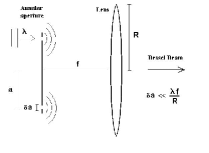
Figure 1: The simple experimental set-up used by Durnin et al. for generating a Bessel beam.

Let us stress, as already mentioned at the end of the previous Subsection, that nowadays a lot of interesting applications of non-diffracting beams are being investigated; besides the Lu et al.’s ones in Acoustics. In the optical sector, let us recall again those of using Bessel beams as optical tweezers able to confine or move around small particles.  In such theoretical and application areas, a noticeable contribution is the one presented in refs.[43-45], wherein, by suitable superpositions of Bessel beams endowed with the same frequency but different longitudinal wavenumbers, stationary envelopes have been mathematically constructed in closed form, which possess a high transverse localization and, more important, a longitudinal intensity-shape that can be freely chosen inside a predetermined space-interval $0\leq z\leq L$. For instance, a high intensity field, with a static envelope, can be created within a tiny region, with negligible intensity elsewhere: As already mentioned, the Third Part will deal, among the others, with such “Frozen Waves”.

Localized (non-diffracting) pulses — As we have seen in the previous Subsection, the existence of non-diffractive (or localized) pulses was predicted since long: cf., once more, refs.[12, 11], and, not less, refs.[9, 13], as well as more recent articles like refs.[46, 47].  The modern studies about non-diffractive pulses (to confine ourselves, at least, to the ones that attracted more attention) followed a development rather independent of those on non-diffracting beams, even if both phenomena are part of the same sector of physics: that of Localized Waves.

In 1983, Brittingham[48] set forth a luminal ($V=c$) solution to the wave equation (more particularly, to the Maxwell equations) which travels rigidly, i.e., without diffraction. The solution proposed in ref.[48] possessed however infinite energy, and once more the problem arose of overcoming such a problem.

A way out was first obtained, as far as we know, by Sezginer[49], who showed how to construct finite-energy luminal pulses, which —however— do not propagate without distortion for an infinite distance, but, as it is expected, travel with constant speed, and approximately without deforming, for a certain (long) depth of field: much longer, in this case too, than that of the ordinary pulses like the gaussian ones. In a series of subsequent papers[30,31,50-53], a simple theoretical method was developed, called by those authors “bidirectional decomposition”, for constructing a new series of non-diffracting luminal pulses.

Eventually, at the beginning of the nineties, Lu et al.[14, 16] constructed, both mathematically and experimentally, new solutions to the wave equation in free space: namely, an X-shaped localized pulse, with the form predicted by the so-called extended Special Relativity[9, 54]; for the connection between what Lu et al. called “X-waves” and “extended” relativity see, e.g., ref.[13], while brief excerpts of that theory can be found, for instance, in refs.[55-58,15].  Lu et al.’s solutions (which can be called the “classic” ones) were continuous superpositions of Bessel beams with the same phase-velocity (i.e., with the same axicon angle[59, 15, 14, 54], $alpha$); so that they could keep their shape for long distances.  Such X-shaped waves resulted to be interesting and flexible localized solutions, and have been afterwards studied in a number of papers, even if their velocity $V$ is supersonic or Superluminal ($V>c$): Actually, when the phase-velocity does not depend on the frequency, it is known that such a phase-velocity becomes the “group-velocity”…  Remembering how a superposition of Bessel beams is generated (for example, by a discrete or continuous set of annular slits or transducers; or even by a single slit plus a lens), it results clear that the energy forming the Localized Waves, coming from those rings, is transported at the ordinary speed $c$ of the plane waves in the considered medium[60-62,15]  (here $c$, representing the velocity of the plane waves in the medium, is the sound-speed in the acoustic case, and the speed of light in the electromagnetic case; and so on).  Nevertheless, the peak of the LWs is faster than $c$.  [Let us explicitly notice that, when using a lens after an aperture located at its back focus, as in Fig.2, then a classic X-shaped pulse can be generated even by a single annular slit, or transducer, illuminated however by a light, or sound, pulse: but the previous considerations about the actual transportation-speed of the “energy” forming the X-shaped wave remain unaffected.  The experimental set-up depicted in Fig.2, with various annular slits, is actually needed only for generating (X-shaped, e.g.) pulses more complex than the classic one, namely, depending on the co-ordinates $z$ and $t$ not only through the quantity $\zeta\equiv z-Vt$: see the following].

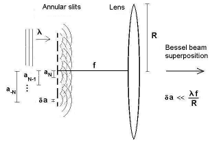
Figure 2: One of the simplest experimental set-ups for generating various kinds of Bessel beam superpositions.

It is indeed possible to generate (besides the “classic” X-wave produced by Lu et al. in 1992) infinite sets of new X-shaped waves, with their energy more and more concentrated in a spot corresponding to the vertex region[38]. It may therefore appear rather intriguing that such a spot [even if no violations of Special Relativity (SR) are obviously implied: all the results come from Maxwell equations, or from the wave equations[63, 64]]— travels Superluminally when the waves are electromagnetic.  For simplicity, we shall call “Superluminal” all the X-shaped waves, even when the waves are acoustic.  By Fig.(3), which refers to an X-wave possessing the velocity $V>c$, we illustrate the fact that, if its vertex or central spot is located at $P_{1}$ at time $t_{1}$, it will reach the position $P_{2}$ at a time $t+\tau$ where $\tau=|P_{2}-P_{1}|/V\;<\;|P_{2}-P_{1}|/c$:  We shall discuss all these points below.

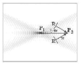
Figure 3: This figure shows an X-shaped wave, that is, a localized Superluminal pulse. It refers to an X-wave, possessing the velocity $V>c$, and illustrates the fact that, if its vertex or central spot is located at $P_{1}$ at time $t_{0}$, it will reach the position $P_{2}$ at a time $t+\tau$ where $\tau=|P_{2}-P_{1}|/V\;<\;|P_{2}-P_{1}|/c$: This is something different from the illusory “scissor effect”, even if the feeding energy, coming from the regions $R$, has travelled with the ordinary speed $c$ (which is the speed of light in the electromagnetic case, or the sound speed in Acoustics, and so on).

Soon after having mathematically and experimentally constructed their “classic” acoustic X-wave, Lu et al. started applying them to ultrasonic scanning, obtaining —as we have already said— very high quality images.  Subsequently, in a 1996 e-print and report, Recami et al. (see, e.g., ref.[15] and refs. therein) published the analogous X-shaped solutions to the Maxwell equations: By constructing scalar Superluminal localized solutions for each component of the Hertz potential. That showed, by the way, that the localized solutions to the scalar equation can be used, under very weak conditions, for obtaining localized solutions to Maxwell’s equations too (actually, Ziolkowski et al.[65] had found something similar, called by them slingshot pulses, for the simple scalar case; but their solution had gone almost unnoticed).  In 1997 Saari et al.[17] announced, in an important paper, the production in the lab of an X-shaped wave in the optical realm, thus proving experimentally the existence of Superluminal electromagnetic pulses.  Three years later, in 2000, Ranfagni et al.[18] produced, in an experiment of theirs, Superluminal X-shaped waves in the microwave region [their paper aroused various criticisms, to which those author however responded].

2 A More Detailed Introduction

Let us refer[66] to the differential equation known as homogeneous wave equation: simple, but so important in Acoustics, Electromagnetism (Microwaves, Optics,…), Geophysics, and even, as we said, gravitational waves and elementary particle physics:

$$\left(\frac{\partial^{2}}{\partial x^{2}}+\frac{\partial^{2}}{\partial y^{2}}+\frac{\partial^{2}}{\partial z^{2}}-\frac{1}{c^{2}}\frac{\partial^{2}}{\partial t^{2}}\right)\,\psi(x,y,z;t)\;=\;0\;.$$ (1)

Let us write it in the cylindrical co-ordinates $(\rho,\phi,z)$ and, for simplicity’s sake, confine ourselves to axially symmetric solutions $\psi(\rho,z;t)$.  Then, eq.(1) becomes

$$\left(\frac{\partial^{2}}{\partial\rho^{2}}+\frac{1}{\rho}\frac{\partial}{\partial\rho}+\frac{\partial^{2}}{\partial z^{2}}-\frac{1}{c^{2}}\frac{\partial^{2}}{\partial t^{2}}\right)\,\psi(\rho,z;t)\;=\;0\ .$$ (2)

In free space, solution $\psi(\rho,z;t)$ can be written in terms of a Bessel-Fourier transform w.r.t. the variable $\rho$, and two Fourier transforms w.r.t. variables $z$ and $t$, as follows:

$$\psi(\rho,z,t)\;=\;\int_{0}^{\infty}\int_{-\infty}^{\infty}\int_{-\infty}^{\infty}\,k_{\rho}\,J_{0}(k_{\rho}\,\rho)\,e^{ik_{z}z}\,e^{-i\omega t}\,\bar{\psi}(k_{\rho},k_{z},\omega)\,{\rm d}k_{\rho}\,{\rm d}k_{z}\,{\rm d}\omega$$ (3)

where $J_{0}(.)$ is an ordinary zero-order Bessel function and $\bar{\psi}(k_{\rho},k_{z},\omega)$ is the transform of $\psi(\rho,z,t)$.

Substituting eq.(3) into eq.(2), one obtains that the relation, among $\omega$, $k_{\rho}$ and $k_{z}\,$,

$$\frac{\omega^{2}}{c^{2}}\;=\;k_{\rho}^{2}+k_{z}^{2}$$ (4)

has to be satisfied.  As a consequence, by using condition (4) in eq.(3), any solution to the wave equation (2) can be written

$$\psi(\rho,z,t)\;=\;\displaystyle{\int_{0}^{\omega/c}\int_{-\infty}^{\infty}\,k_{\rho}\,J_{0}(k_{\rho}\,\rho)\,e^{i\sqrt{\omega^{2}/c^{2}\,-\,k_{\rho}^{2}}\,\,z}\,e^{-i\omega t}\,S(k_{\rho},\omega)\,{\rm d}k_{\rho}\,{\rm d}\omega}$$ (5)

where $S(k_{\rho},\omega)$ is the chosen spectral function, when $k_{z}>0$ (and we disregard evenescent waves).

The general integral solution (5) yields for instance the (non-localized) gaussian beams and pulses, to which we shall refer for illustrating the differences of the localized waves w.r.t. them.

The Gaussian Beam — A very common (non-localized) beam is the gaussian beam[67], corresponding to the spectrum

$$S(k_{\rho},\omega)\;=\;2a^{2}\,e^{-a^{2}k_{\rho}^{2}}\,\delta(\omega-\omega_{0})\;.$$ (6)

In eq.(6), $a$ is a positive constant, which will be shown to depend on the transverse aperture of the initial pulse.

Figure 4 illustrates the interpretation of the integral solution (5), with spectral function (6), as a superposition of plane waves.  Namely, from Fig.4 one can easily realize that this case corresponds to plane waves propagating in all directions (always with $k_{z}\geq 0$), the most intense ones being those directed along (positive) $z$. Notice that, in the plane-wave case, $\vec{k_{z}}$ is the longitudinal component of the wave-vector, $\vec{k}=\vec{k_{\rho}}+\vec{k_{z}}$, where $\vec{k_{\rho}}=\vec{k_{x}}+\vec{k_{y}}$.

Figure 4: Visual interpretation of the integral solution (5), with spectral function (6), in terms of a superposition of plane waves.

On substituting eq.(6) into eq.(5) and adopting the paraxial approximation, one meets the gaussian beam

$$\psi_{\rm gauss}(\rho,z,t)\;=\;\frac{\displaystyle{2a^{2}\,{\rm exp}\left(\displaystyle{\frac{-\rho^{2}}{4(a^{2}+i\,z/2k_{0})}}\right)}}{\displaystyle{2(a^{2}+i\,z/2k_{0})}}\,\,\displaystyle{e^{ik_{0}(z-ct)}}\;\;,$$ (7)

where $k_{0}=\omega_{0}/c$. We can verify that such a beam, which suffers transverse diffraction, doubles its initial width $\Delta\rho_{0}=2a$ after having travelled the distance $z_{{\rm dif}}\;=\;\sqrt{3}\,k_{0}\Delta\rho_{0}^{2}/2$, called diffraction length. The more concentrated a gaussian beam happens to be, the more rapidly it gets spoiled.

The Gaussian Pulse — The most common (non-localized) pulse is the gaussian pulse, which is got from eq.(5) by using the spectrum[68]

$$S(k_{\rho},\omega)\;=\;\frac{2ba^{2}}{\sqrt{\pi}}e^{-a^{2}k_{\rho}^{2}}e^{-b^{2}(\omega-\omega_{0})^{2}}$$ (8)

where $a$ and $b$ are positive constants. Indeed, such a pulse is a superposition of gaussian beams of different frequency.

Now, on substituting eq.(8) into eq.(5), and adopting once more the paraxial approximation, one gets the gaussian pulse:

$$\psi(\rho,z,t)\;=\;\frac{a^{2}\,{\rm exp}\left(\displaystyle{\frac{-\rho^{2}}{4(a^{2}+iz/2k_{0})}}\right){\rm exp}\left(\displaystyle{\frac{-(z-ct)^{2}}{4c^{2}b^{2}}}\right)}{a^{2}+iz/2k_{0}}\;\;,$$ (9)

endowed with speed $c$ and temporal width $\Delta t=2b$, and suffering a progressing enlargement of its transverse width, so that its initial value gets doubled already at position $z_{{\rm dif}}\;=\;\sqrt{3}\,k_{0}\Delta\rho_{0}^{2}/2\;$,  with $\Delta\rho_{0}=2a$.

2.1 The localized solutions

Let us finally go on to the construction of the two most renowned localized waves[66]: the Bessel beam, and the ordinary X-shaped pulse.

First of all, it is interesting to observe that, when superposing (axially symmetric) solutions of the wave equation in the vacuum, three spectral parameters, $(\omega,\ k_{\rho},\ k_{z})$, come into the play, which have however to satisfy the constraint (4), deriving from the wave equation itself. Consequently, only two of them are independent: and we choose here $\omega$ and $k_{\rho}$.  Such a possibility of choosing $\omega$ and $k_{\rho}$ was already apparent in the spectral functions generating gaussian beams and pulses, which consisted in the product of two functions, one depending only on $\omega$ and the other on $k_{\rho}$.

We are going to see that further particular relations between $\omega$ and $k_{\rho}$ [or, analogously, between $\omega$ and $k_{z}$] can be moreover enforced, in order to get interesting and unexpected results, such as the localized waves.

The Bessel beam — Let us start by imposing a linear coupling between $\omega$ and $k_{\rho}$ (it could be actually shown[37] that it is the unique coupling leading to localized solutions).

Namely, let us consider the spectral function

$$S(k_{\rho},\omega)\;=\;\frac{\delta(k_{\rho}-\displaystyle{\frac{\omega}{c}}\sin\theta)}{k_{\rho}}\,\,\delta(\omega-\omega_{0})\;\;,$$ (10)

which implies that $k_{\rho}=(\omega\sin\theta)/c$,  with $0\leq\theta\leq\pi/2$:  A relation that can be regarded as a space-time coupling. Let us add that this linear constraint between $\omega$ and $k_{\rho}$, together with relation (4), yields  $k_{z}=(\omega\cos\theta)/c$. This is an important fact, since it has been shown elsewhere[66, 38] that an ideal localized wave must contain a coupling of the type $\omega=Vk_{z}+b$, where $V$ and $b$ are arbitrary constants.

The interpretation of the integral function (5), this time with spectrum (10), as a superposition of plane waves is visualized in Figure 5: which shows that an axially-symmetric Bessel beam is nothing but the result of the superposition of plane waves whose wave vectors lay on the surface of a cone having the propagation line as its symmetry axis and an opening angle equal to $\theta$; such $\theta$ being called the axicon angle.

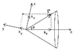
Figure 5: The axially-symmetric Bessel beam is created by the superposition of plane waves whose wave vectors lay on the surface of a cone having the propagation axis as its symmetry axis and angle equal to $\theta$ (”axicon angle”).

By inserting eq.(10) into eq.(5), one gets the mathematical expression of the so-called Bessel beam:

$$\psi(\rho,z,t)\;=\;J_{0}\left(\frac{\omega_{0}}{c}\sin\theta\,\,\rho\right)\,{\rm exp}\left[i\,\,\frac{\omega_{0}}{c}\cos\theta\,\left(z-\frac{c}{\cos\theta}t\right)\right]\;.$$ (11)

This beam possesses phase-velocity $v_{\rm ph}=c/\cos\theta$, and field transverse shape represented by a Bessel function $J_{0}(.)$ so that its field in concentrated in the surroundings of the propagation axis $z$. Moreover, eq.(11) tells us that the Bessel beam keeps its transverse shape (which is therefore invariant) while propagating, with central “spot” $\Delta\rho=2.405c/(\omega\sin\theta)$.

The ideal Bessel beam, however, is not square-integrable in the transverse direction, and is therefore associated with an infinite power flux:  i.e., it cannot be experimentally produced.

But we can have recourse to truncated Bessel beams, generated by finite apertures. In this case the (truncated) Bessel beams are still able to travel a long distance while maintaining their transfer shape, as well as their speed, approximately unchanged[36, 69, 70]: That is to say, they still possess a large depth of field. For instance, the field-depth of a Bessel beam generated by a circular finite aperture with radius $R$ is given by

$$Z_{\rm max}\;=\;\frac{R}{\tan\theta}\;,$$ (12)

where $\theta$ is the beam axicon angle. In the finite aperture case, the Bessel beam cannot be represented any longer by eq.(11), and one has to calculate it by the scalar diffraction theory: By using, for example, Kirchhoff’s or Rayleigh-Sommerfeld’s diffraction integrals. But till the distance $Z_{\rm max}$ one may still use eq.(11) for approximately describing the beam, at least in the vicinity of the axis $\rho=0$, that is, for $\rho<<R$. To realize how much a truncated Bessel beam succeeds in resisting diffraction, let us consider also a gaussian beam, with the same frequency and central “spot”, and compare their field-depths. In particular, let us assume for both beams $\lambda=0.63\;\mu$m and initial central “spot” size $\Delta\rho_{0}=60\;\mu$m. The Bessel beam will possess axicon angle $\theta=\arcsin[2.405c/(\omega\Delta\rho_{0})]=0.004\;$rad. Figure 6 depicts the behaviour of the two beams for a circular aperture with radius $3.5\;$mm.  We can verify how the gaussian beam doubles its initial transverse width already after $3\;$cm, and after $6\;$cm its intensity has become an order of magnitude smaller. By contrast, the truncated Bessel beam keeps its transverse shape until the distance $Z_{\rm max}=R/\tan\theta=85\;$cm. Afterwards, the Bessel beam rapidly decays, as a consequence of the sharp cut performed on its aperture (such cut being responsible also for the intensity oscillations suffered by the beam along its propagation axis, and for the fact that eventually the feeding waves, coming from the aperture, at a certain point get faint).

Figure 6: Comparison between a gaussian (a) and a truncated Bessel beam (b). One can see that the gaussian beam doubles its initial transverse width already after $3\;$cm, while after $6\;$cm its intensity decays of a factor 10. By contrast, the Bessel beam does approximately keep its transverse shape till the distance $85\;$cm.

The zeroth-order (axially symmetric) Bessel beam is nothing but one example of localized beam. Further examples are the higher order (not cylindrically symmetric) Bessel beams

$$\psi(\rho,\phi,z;t)\;=\;J_{\nu}\left(\frac{\omega_{0}}{c}\sin\theta\,\,\rho\right)\,{\rm exp}(i\nu\phi)\;{\rm exp}\left(i\,\,\frac{\omega_{0}}{c}\cos\theta\,\left(z-\frac{c}{\cos\theta}t\right)\right)\;\;,$$ (13)

or the Mathieu beams[71], and so on.

The Ordinary X-shaped Pulse — Following the same procedure adopted in the previous subsection, let us construct pulses by using spectral functions of the type

$$S(k_{\rho},\omega)\;=\;\frac{\delta(k_{\rho}-\displaystyle{\frac{\omega}{c}}\sin\theta)}{k_{\rho}}\,\,F(\omega)\;,$$ (14)

where this time the Dirac delta function furnishes the spectral space-time coupling $k_{\rho}=(\omega\sin\theta)/c$.  Function $F(\omega)$ is, of course, the frequency spectrum; it is left for the moment undetermined.

On using eq.(14) into eq.(5), one obtains

$$\psi(\rho,z,t)\;=\;\int_{-\infty}^{\infty}\,F(\omega)\,J_{0}\left(\frac{\omega}{c}\sin\theta\,\,\rho\right)\,{\rm exp}\left(\frac{\omega}{c}\cos\theta\,\left(z-\frac{c}{\cos\theta}t\right)\right)\,{\rm d}\omega\ .$$ (15)

It is easy to see that $\psi$ will be a pulse of the type

$$\psi\;=\;\psi(\rho,z-Vt)$$ (16)

with a speed $V=c/\cos\theta$ independent of the frequency spectrum $F(\omega)$.

Such solutions are known as X-shaped pulses, and are localized (non-diffractive) waves in the sense that they do obviously maintain their spatial shape during propagation (see., e.g., refs.[14, 15, 38] and refs. therein; as well as the following).

At this point, some remarkable observations are to be stressed:

(i) When a pulse consists in a superposition of waves (in this case, Bessel beams) all endowed with the same phase-velocity $V_{\rm ph}$ (in this case, with the same axicon angle) independent of their frequency, then it is known that the phase-velocity (in this case $V_{\rm ph}=c/\cos\theta$) becomes[72, 73] the group-velocity $V$: That is, $V=c/\cos\theta>c$. In this sense, the X-shaped waves are called “Superluminal localized pulses” (cf., e.g., ref.[15] and refs. therein).  [For simplicity, the group-velocity we are talking about[38, 57, 93, 57] can be regarded as the peak-velocity.  Here, let us only add the observations:  (a) that the group-velocity for a pulse, in general, is well defined only when the pulse has a clear bump in space; but it can be calculated by the approximate, simple relation  $V\simeq{\rm d}\omega/{\rm d}k$  only when some extra conditions are satisfied (namely, when $\omega$ as a function of $k$ is also clearly bumped);  and  (b) that the group velocity can a priori be evaluated through the mentioned, customary derivation of $\omega$ with respect to the wavenumber for the infinite total energy solutions; whilst, for the finite total energy Superluminal solutions, the group-velocity cannot be calculated through such an elementary relation, since in those cases it does not even exist a one-to-one function $\omega=\omega(k_{z})$].

(ii) Such pulses, even if their group-velocity is Superluminal, do not contradict standard physics, having been found in what precedes on the basis of the wave equations —in particular, of Maxwell equations[30, 15]— only. Indeed, as we shall better see in the historical Appendix following below at the end of the First Part, their existence can be understood within Special Relativity itself[9,13,15,55-57], on the basis of its ordinary Postulates[54]. Actually, let us repeat it once more, they are fed by waves originating at the aperture and carrying energy with the standard speed $c$ of the medium (the light-velocity in the electromagnetic case, and the sound-velocity in the acoustic[16] case).  We can become convinced about the possibility of realizing Superluminal X-shaped pulses by imagining the simple ideal case of a negligibly sized Superluminal source $S$ endowed with speed $V>c$ in vacuum, and emitting electromagnetic waves $W$ (each one travelling with the invariant speed $c$). The electromagnetic waves will result to be internally tangent to an enveloping cone $C$ having $S$ as its vertex, and as its axis the propagation line $z$ of the source[54, 13]: This is completely analogous to what happens for an airplane that moves in air with constant supersonic speed.  The waves $W$ interfere mainly negatively inside the cone $C$, and constructively on its surface.  We can place a plane detector orthogonally to $z$, and record magnitude and direction of the $W$ waves that hit on it, as (cylindrically symmetric) functions of position and of time.  It will be enough, then, to replace the plane detector with a plane antenna which emits —instead of recording— exactly the same (axially symmetric) space-time pattern of waves $W$, for constructing a cone-shaped electromagnetic wave $C$ that will propagate with the Superluminal speed $V$ (of course, without a source any longer at its vertex…):  even if each wave $W$ travels with the invariant speed $c$.  Once more, this is exactly what would happen in the case of a supersonic airplane (in which case $c$ is the sound speed in air: for simplicity, assume the observer to be at rest with respect to the air).  For further details, see the quoted references.  Actually, by suitable superpositions, and interference, of speed-$c$ waves, one can obtain pulses more and more localized in the vertex region[38]: That is, very localized field-“blobs” which travels with Superluminal group-velocity.  This has nothing to do apparently with the illusory “scissors effect”, since such blobs, along their field-depth, are a priori able, e.g., to get two successive (weak) detectors, located at a distance $L$, to click after a time smaller than $L/c$. Incidentally, an analysis of the above-mentioned case (that of a supersonic plane or a Superluminal charge) led, as expected[54], to the simplest type of “X-shaped pulse”[13].  It might be useful, finally, to recall that SR (even the wave-equations have an internal relativistic structure!) implies considering also the forward cone: cf. Fig.7. The truncated X-waves considered in this paper, for instance, must have a leading cone in addition to the rear cone; such a leading cone having a role for the peak stability[14]: For example, in the approximate case in which we produce a finite conic wave truncated both in space and in time, the theory of SR suggested the bi-conic shape (symmetrical in space with respect to the vertex $S$) to be a better approximation to a rigidly travelling wave (so that SR suggests to have recourse to a dynamic antenna emitting a radiation cylindrically symmetric in space and symmetric in time, for a better approximation to an “undistorted progressing wave”).

Figure 7: The truncated X-waves considered in this paper, as predicted by SR (all wave-equations have an intrinsic relativistic structure!), must have a leading cone in addition to the rear cone; such a leading cone having a role for the peak stability[14]: For example, when producing a finite conic wave truncated both in space and in time, the theory of SR suggested to have recourse, in the simplest case, to a dynamic antenna emitting a radiation cylindrically symmetrical in space and symmetric in time, for a better approximation to what Courant and Hilbert[11] called an “undistorted progressing wave”. See the following, in the text.

(iii) Any solutions that depend on $z$ and on $t$ only through the quantity $z-Vt$, like eq.(15), will appear with a constant shape to an observer travelling along $z$ with the speed $V$. That is, such a solution will propagate rigidly with speed $V$. This does further explain why our X-shaped pulses, after having been produced, will travel almost rigidly at speed $V$ (in this case, a faster-than-light group-velocity), all along their depth of field.  To be even clearer, let us consider a generic function, depending on $z-Vt$ with $V>c$, and show, by explicit calculations involving the Maxwell equations only, that it obeys the scalar wave equation.  Following Franco Selleri[74], let us consider, e.g., the wave function

$$\Phi(x,y,z,t)\;=\;{\displaystyle{\frac{a}{{\sqrt{[b-ic(z-Vt)]^{2}+(V^{2}-c^{2})(x^{2}+y^{2})}}}}}$$ (17)

with $a$ and $b$ non-zero constants, $c$ the ordinary speed of light, and $V>c$  [incidentally, this wave function is nothing but the classic X-shaped wave in cartesian co-ordinates]. Let us naively verify that it is a solution to the wave equation

$$\mbox{\boldmath$\nabla$}^{2}\Phi(x,y,z,t)-{\frac{1}{c^{2}}}\;{\frac{\partial^{2}\Phi(x,y,z,t)}{\partial^{2}t}}\;=\;0\ .$$ (18)

On putting

$$R\,\equiv\,\displaystyle{{{\sqrt{[b-ic(z-Vt)]^{2}+(V^{2}-c^{2})(x^{2}+y^{2})}}}}\;,$$ (19)

one can write $\Phi=a/R$ and evaluate the second derivatives

$$\frac{1}{a}\,\frac{\partial^{2}\Phi}{\partial^{2}z}\;=\;\frac{c^{2}}{R^{3}}-\frac{3c^{2}}{R^{5}}\,[b-ic(z-Vt)]^{2}\ ;$$

$$\frac{1}{a}\,\frac{\partial^{2}\Phi}{\partial^{2}x}\;=\;-\frac{V^{2}-c^{2}}{R^{3}}\,+\,3\left(V^{2}-c^{2}\right)^{2}\;\frac{x^{2}}{R^{5}}\ ;$$

$$\frac{1}{a}\,\frac{\partial^{2}\Phi}{\partial^{2}y}\;=\;-\frac{V^{2}-c^{2}}{R^{3}}\,+\,3\left(V^{2}-c^{2}\right)^{2}\;\frac{y^{2}}{R^{5}}\;$$

$$\frac{1}{a}\,\frac{\partial^{2}\Phi}{\partial^{2}t}\;=\;\frac{c^{2}V^{2}}{R^{3}}-\frac{3c^{2}V^{2}}{R^{5}}\,[b-ic(z-Vt)]^{2}\ ;$$

wherefrom

$$\frac{1}{a}\,\left[\frac{\partial^{2}\Phi}{\partial^{2}z}-\frac{1}{c^{2}}\frac{\partial^{2}\Phi}{\partial^{2}t}\right]\;=\;-\frac{V^{2}-c^{2}}{R^{3}}+3\left(V^{2}-c^{2}\right)^{2}\;\frac{[b-ic(z-Vt)]^{2}}{R^{5}}\ ,$$

and

$$\frac{1}{a}\,\left[\frac{\partial^{2}\Phi}{\partial^{2}x}+\frac{\partial^{2}\Phi}{\partial^{2}y}\right]\;=\;-2\,\frac{V^{2}-c^{2}}{R^{3}}+3\left(V^{2}-c^{2}\right)^{2}\;\frac{x^{2}+y^{2}}{R^{5}}\ .$$

From the last two equations, remembering the previous definition, one finally gets

$$\frac{1}{a}\,\left[{\frac{\partial^{2}\Phi}{\partial^{2}z}}+{\frac{\partial^{2}\Phi}{\partial^{2}x}}+{\frac{\partial^{2}\Phi}{\partial^{2}y}}-{\frac{1}{c^{2}}}\;{\frac{\partial^{2}\Phi}{\partial^{2}t}}\right]\;=\;0$$

that is nothing but the (d’Alembert) wave equation (18), q.e.d.   In conclusion, function $\Phi$ is a solution of the wave equation even if it does obviously represent a pulse (Selleri says “a signal”!) propagating with Superluminal speed.

At this point, the reader should be however warned that all the subluminal LWs, solutions of the ordinary homogeneous wave equation, have appeared till now to present sungularities whenever they depend on $z$ and $t$ only via the quantity $\zeta\equiv z-Vt$:  This is still an open, interesting research topic, which is related also to analogous results met in gravitation physics.

After the previous three important comments, let us go back to our evaluations with regard to the X-type solutions to the wave equations.  Let us now consider in eq.(15), for instance, the particular frequency spectrum $F(\omega)$ given by

$$F(\omega)\;=\;H(\omega)\,\frac{a}{V}\,\,\,{\rm exp}\left(-\frac{a}{V}\,\omega\right)\;,$$ (20)

where $H(\omega)$ is the Heaviside step-function and $a$ a positive constant. Then, eq.(15) yields

$$\psi(\rho,\zeta)\,\equiv\,X\;=\;\frac{a}{\sqrt{(a-i\zeta)^{2}+\left(\frac{V^{2}}{c^{2}}-1\right)\rho^{2}}}\;,$$ (21)

with $\zeta\equiv z-Vt$. This solution (21) is the well-known ordinary, or “classic”, X-wave, which constitutes a simple example of X-shaped pulse.[14, 15]  Notice that function (20) contains mainly low frequencies, so that the classic X-wave is suitable for low frequencies only.

Figure 8 depicts (the real part of) an ordinary X-wave with $V=1.1\,c$ and $a=3\;$m.

Figure 8: Plot of the real part of the ordinary X-wave, evaluated for $V=1.1\,c$ with $a=3\;$m .

Solutions (15), and in particular the pulse (21), have got an infinite field-depth, and an infinite energy as well. Therefore, as it was done in the Bessel beam case, one should pass to truncated pulses, originating from a finite aperture. Afterwards, our truncated pulses will keep their spatial shape (and their speed) all along the depth of field

$$Z\;=\;\frac{R}{\tan\theta}\;,$$ (22)

where, as before, $R$ is the aperture radius and $\theta$ the axicon angle.

Some Further Observations — Let us put forth some further observations.

It is not strictly correct to call non-diffractive the localized waves, since diffraction affects, more or less, all waves obeying eq.(1). However, all localized waves (both beams and pulses) possess the remarkable “self-reconstruction” property: That is to say, the localized waves, when diffracting during propagation, do immediately re-build their shape[39-41] (even after obstacles with size much larger than the characteristic wave-lengths, provided it is smaller —as we know— than the aperture size), due to their particular spectral structure [as it is shown more in detail, e.g., in the book Localized Waves (J.Wiley; Jan.2008)]. In particular, the “ideal localized waves” (with infinite energy and field-depth) are able to re-build themselves for an infinite time; while, as we have seen, the finite-energy (truncated) ones can do it, and thus resist the diffraction effects, only along a certain depth of field…

Let us stress again that the interest of the localized waves (especially from the point of view of applications) lies in the circumstance that they are almost non-diffractive, rather than in their group-velocity: From this point of view, Superluminal, luminal, and subluminal localized solutions are equally interesting and suited to important applications.

Actually, the localized waves are not restricted to the (X-shaped, Superluminal) ones corresponding to the integral solution (15) to the wave equation; and, as we were already saying, three classes of localized pulses exist: the Superluminal (with speed $V>c$), the luminal ($V=c$), and the subluminal ($V<c$) ones; all of them with, or without, axial symmetry, and corresponding in any case to a single, unified mathematical background.  This issue will be touched again in the present review.

Incidentally, we have addressed elsewhere topics  as: (i) the construction of infinite families of generalizations of the classic X-shaped wave [with energy more and more concentrated around the vertex: cf., e.g., Figs.9, taken from ref.[38]]; as  (ii) the behaviour of some finite total-energy Superluminal localized solutions (SLS);  (iii) the techniques for building up new series of SLS’s to the Maxwell equations suitable for arbitrary frequencies and bandwidths;  (iv) questions related with the case of dispersive (and even lossy) media;  (v) the construction of (infinite or finite energy) Superluminal LWs propagating down waveguides or coaxial cables;  (vi) finding out Localized Solutions also to equations different from the wave equation, as Schroedinger’s;  (vii) using the above tecniques for constructing, in General Relativity, new exact solutions for gravitational ways.   In the Second Part of this paper we shall come back to some (few) of those points.  Let us add that X-shaped waves have been easily produced also in nonlinear media[75].

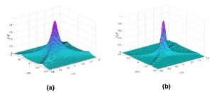
Figure 9: In Fig.(a) it is represented (in arbitrary units) the square magnitude of the “classic”, $X$-shaped Superluminal localized solution (SLS) to the wave equation, with $V=5c$ and $a=0.1\;$m.  Families of infinite SLSs however exists, which generalize the classic $X$-shaped solution; for instance, a family of SLSs obtained[38] by suitably differentiating the classic X-wave: Fig.(b) depicts the first of them (corresponding to the first differentiation) with the same parameters.  As we said, the successsive solutions in such a family are more and more localized around their vertex. Quantity $\rho$ is the distance in meters from the propagation axis $z$, while quantity $\zeta$ is the “$V$-cone” variable[ref.[38]] (still in meters) $\zeta\equiv z-Vt$, with $V\geq c$.  Since all these solutions depend on $z$ only via the variable $\zeta$, they propagate “rigidly”, i.e., as we know, without distortion (and are called “localized”, or non-diffracting, for such a reason). Here we are assuming propagation in the vacuum (or in a homogeneous medium).

A more technical introduction to the subject of localized waves (particularly w.r.t. the Superluminal X-shaped ones) can be found in the Second Part of this review, and in papers like ref.[55].

Before going on to the Second Part of this paper, let us end the present First Part by a historical (theoretical and experimental) Appendix.

An APPENDIX to the First Part:

A HISTORICAL (THEORETICAL AND EXPERIMENTAL)

APPENDIX

In this mainly “historical” Appendix, written as far as possible in a (partially) self-consistent form, we shall first refer ourselves, from the theoretical point of view, to the most intriguing localized solutions to the wave equation: the Superluminal ones (SLS), and in particular the X-shaped pulses. As a start, we shall recall their geometrical interpretation within SR. Afterwards, to help resolving possible doubts, we shall seize the opportunity, given by this Appendix, for presenting a bird’s-eye view of the various experimental sectors of physics in which Superluminal motions seem to appear: In particular, of the experiments with evanescent waves (and/or tunnelling photons), and with the SLS’s we are more interested in here. In some parts of this Appendix the propagation-line is called $x$, and no longer $z$, without originating, however, any interpretation problems.

3 An Introduction to the APPENDIX

The question of Superluminal ($V^{2}>c^{2}$) objects or waves has a long story. Still in pre-relativistic times, one meets various relevant papers, from those by J.J.Thomson to the interesting ones by A.Sommerfeld. It is well-known, however, that with SR the conviction spread out that the speed $c$ of light in vacuum was the upper limit of any possible speed. For instance, R.C.Tolman in 1917 believed to have shown by his “paradox” that the existence of particles endowed with speeds larger than $c$ would have allowed sending information into the past.  Our problem started to be tackled again only in the fifties and sixties, in particular after the papers[76] by E.C.George Sudarshan et al., and, later on[77, 78], by one of the present authors with R.Mignani et al., as well as —to confine ourselves at present to the theoretical researches— by H.C.Corben and others. The first experimental attempts were performed by T.Alväger et al.

We wish to face the still unusual issue of the possible existence of Superluminal wavelets, and objects —within standard physics and SR, as we said— since at least four different experimental sectors of physics seem to support such a possibility [apparently confirming some long-standing theoretical predictions[54, 9, 76, 78]]. The experimental review will be necessarily short, but we shall provide the reader with enough bibliographical information, limited for brevity’s sake to the last century only (i.e., up-dated till the year 2000 only).

4 APPENDIX: Historical Recollections - Theory

A simple theoretical framework was long ago proposed[76, 54, 77], merely based on the space-time geometrical methods of SR, which appears to incorporate Superluminal waves and objects, and in a sense predicts[9] among the others the Superluminal X-shaped waves, without violating the Relativity principles. A suitable choice of the Postulates of SR (equivalent of course to the other, more common, choices) is the following one: (i) the standard Principle of Relativity; and (ii) space-time homogeneity and space isotropy.  It follows that one and only one invariant speed exists; and experience shows that invariant speed to be the light-speed, $c$, in vacuum: The essential role of $c$ in SR being just due to its invariance, and not to the fact that it be a maximal, or minimal, speed. No sub- or Super-luminal objects or pulses can be endowed with an invariant speed: so that their speed cannot play in SR the same essential role played the light-speed $c$ in vacuum. Indeed, the speed $c$ turns out to be also a limiting speed: but any limit possesses two sides, and can be approached a priori both from below and from above: See Fig.10.  As E.C.G.Sudarshan put it, from the fact that no one could climb over the Himalayas ranges, people of India cannot conclude that there are no people North of the Himalayas… Indeed, speed-$c$ photons exist, which are born, live and die just “at the top of the mountain,” without any need for performing the impossible task of accelerating from rest to the light-speed.  [Actually, the ordinary formulation of SR has been too much restricted: For instance, even leaving Superluminal speeds aside, it can be easily so widened as to include antimatter[54, 58, 57]].

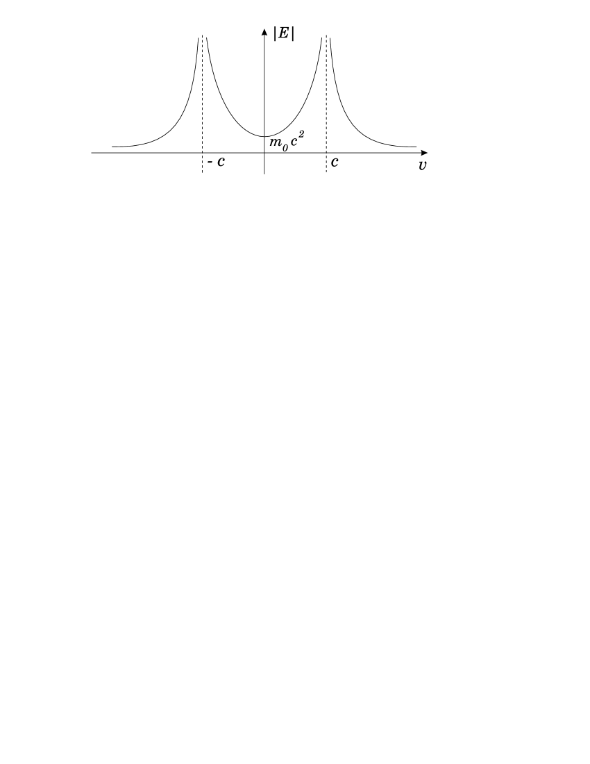
Figure 10: Energy of a free object as a function of its speed.[76, 77, 54]

An immediate consequence is that the quadratic form  $c^{2}{\rm d}t^{2}-{\rm d}\mbox{\boldmath$x$}^{2}\equiv{\rm d}x_{\mu}{\rm d}x^{\mu}$, called ${\rm d}s^{2}$,  with ${\rm d}\mbox{\boldmath$x$}^{2}\equiv{\rm d}x^{2}+{\rm d}y^{2}+{\rm d}z^{2}$,  results to be invariant, except for its sign.  Quantity ${\rm d}s^{2}$, let us recall, is the four-dimensional length-element square, along the space-time path of any object.  In correspondence with the positive (negative) sign, one gets the subluminal (Superluminal) Lorentz “transformations” [LT]. More specifically, the ordinary subluminal LTs are known to leave, e.g., the quadratic forms ${\rm d}x_{\mu}{\rm d}x^{\mu}$, ${\rm d}p_{\mu}{\rm d}p^{\mu}$ and ${\rm d}x_{\mu}{\rm d}p^{\mu}$ exactly invariant, where the $p_{\mu}$ are the component of the energy-impulse four-vector; while the Superluminal LTs, by contrast, have to change (only) the sign of such quadratic forms. This is enough for deducing some important consequences, like the one that a Superluminal charge has to behave as a magnetic monopole, in the sense specified in ref.[54] and refs. therein.

A more important consequence, for us, is —see Fig.11— that the simplest subluminal object, namely a spherical particle at rest (which appears as ellipsoidal, due to Lorentz contraction, at subluminal speeds $v$), will appear[9, 54, 15] as occupying the cylindrically symmetrical region bounded by a two-sheeted rotation hyperboloid and an indefinite double cone, as in Fig.(11d), for Superluminal speeds $V$. In the limiting case of a point-like particle, one obtains only a double cone.

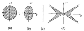
Figure 11: An intrinsically spherical (or pointlike, at the limit) object appears in the vacuum as an ellipsoid contracted along the motion direction when endowed with a speed $v<c$.  By contrast, if endowed with a speed $V>c$ (even if the $c$-speed barrier cannot be crossed, neither from the left nor from the right), it would appear[9, 54] no longer as a particle, but rather as an “X-shaped” wave travelling rigidly: Namely, as occupying the region delimited by a double cone and a two-sheeted hyperboloid —or as a double cone, at the limit–, and moving without distortion in the vacuum, or in a homogeneous medium, with Superluminal speed $V$ [the square cotangent of the cone semi-angle being $(V/c)^{2}-1$]. For simplicity, a space axis is skipped.  This figure is taken from refs.[9, 54].

Such a result is got by writing down the equation of the world-tube of a subluminal particle, and transforming it simply by changing the sign of the quadratic forms entering that equation. Thus, in 1980-1982, it was predicted[9] that the simplest Superluminal object appears (not as a particle, but as a field or rather) as a wave: namely, as an “X-shaped pulse”, the cone semi-angle $\alpha$ being given (with $c=1$) by  ${\rm cotg}\,\alpha=\sqrt{V^{2}-1}$. Such X-shaped pulses will move rigidly with speed $V$ along their motion direction: In fact, any “X-pulse” can be regarded at each instant of time as the (Superluminal) Lorentz transform of a spherical object, which of course moves in vacuum —or in a homogeneous medium— without any deformation as time elapses.  The three-dimensional picture of Fig.(11d) appears in Fig.12, where its annular intersections with a transverse plane are shown (cf. refs.[9]).  The X-shaped waves here considered are merely the simplest ones: if one starts not from an intrinsically spherical or point-like object, but from a non-spherically symmetric particle, or from a pulsating (contracting and dilating) sphere, or from a particle oscillating back and forth along the motion direction, then their Superluminal Lorentz transforms would result to be more and more complicated. The above-seen “X-waves”, however, are typical for a Superluminal object, as much as the spherical or point-like shape is typical, let us repeat, for a subluminal object.

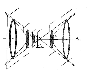
Figure 12: Here we show the intersections of the Superluminal object $T$ represented in Fig.(11d) with planes $P$ orthogonal to its motion line (the $z$-axis).  For simplicity, we assumed again the object to be spherical in its rest-frame, and the cone vertex $C$ to coincide with the origin $O$ for $t=0$.  Such intersections evolve in time so that the same pattern appears on a second plane —shifted by $\Delta x$— after the time $\Delta t=\Delta x/V$.  On each plane, as time elapses, the intersection is therefore predicted by (extended) SR to be a circular ring which, for negative times, goes on shrinking until it reduces to a circle and then to a point (for $t=0$);  afterwards, such a point becomes again a circle and then a circular ring that goes on broadening[9, 54, 15].  This picture is taken from refs.[9, 54].  [Notice that, if the object is not spherical when at rest (but, e.g., is ellipsoidal in its own rest-frame), then the axis of $T$ will no longer coincide with $x$, but its direction will depend on the speed $V$ of the tachyon itself].  For the case in which the space extension of the Superluminal object $T$ is finite, see refs.[9]

Incidentally, it has been believed for a long time that Superluminal objects would have allowed sending information into the past; but such problems with causality seem to be solvable within SR. Once SR is generalized in order to include Superluminal objects or pulses, no signal travelling backward in time is apparently left. For a solution of those causal paradoxes, see refs.[58, 57, 76] and references therein.

When addressing the problem, within this elementary Appendix, of the production of an X-shaped pulse like the one depicted in Fig.12 (maybe truncated, in space and in time, by use of a finite antenna radiating for a finite time), all the considerations expounded under point (ii) of the subsection The Ordinary X-shaped Pulse become in order: And, here, we simply refer to them. Those considerations, together with the present ones (related, e.g., to Fig.12), suggest the simplest antenna to consist in a series of concentric annular slits, or transducers [like in Fig.2], which suitably radiate following specific time patterns: See, e.g., refs.[79] and refs. therein.  Incidentally, the above procedure can lead to a very simple type of X-shaped wave, as investigated below.

From the present point of view, it is rather interesting to note that, during the last fifteen years, X-shaped waves have been actually found as solutions to the Maxwell and to the wave equations [let us repeat that the form of any wave equations is intrinsically relativistic]. In order to see more deeply the connection existing between what predicted by SR (see, e.g., Figs.11,12) and the localized X-waves mathematically, and experimentally, constructed in recent times, let us tackle below, in detail, the problem of the (X-shaped) field created by a Superluminal electric charge[13], by following a paper recently appeared in Physical Review E.

4.1 The particular X-shaped field associated with a Superluminal charge

It is well-known by now that Maxwell equations admit of wavelet-type solutions endowed with arbitrary group-velocities ($0<v_{\rm g}<\infty$).  We shall again confine ourselves, as above, to the localized solutions, rigidly moving: and, more in particular, to the Superluminal ones (SLS), the most interesting of which resulted to be X-shaped, as we have already seen.  The SLSs have been actually produced in a number of experiments, always by suitable interference of ordinary-speed waves.  In this subsection we show, by contrast, that even a Superluminal charge creates an electromagnetic X-shaped wave, in agreement with what predicted[9, 54] within SR. In fact, on the basis of Maxwell equations, one is able to evaluate the field associated with a Superluminal charge (at least, under the rough approximation of pointlikeness): As announced in what precedes, it results to constitute a very simple example of true X-wave.

Indeed, the theory of SR, when based on the ordinary Postulates but not restricted to subluminal waves and objects, i.e., in its extended version, predicted the simplest X-shaped wave to be the one corresponding to the electromagnetic field created by a Superluminal charge[80, 13].  It seems really important evaluating such a field, at least approximately, by following ref.[13].

The toy-model of a pointlike Superluminal charge — Let us start by considering, formally, a pointlike Superluminal charge, even if the hypothesis of pointlikeness (already unacceptable in the subluminal case) is totally inadequate in the Superluminal case[54].  Then, let us consider the ordinary vector-potential $A^{\mu}$ and a current density $j^{\mu}\equiv(0,0,j_{z};j^{\rm o})$ flowing in the $z$-direction (notice that the motion line is still the axis $z$). On assuming the fields to be generated by the sources only, one has that $A^{\mu}\equiv(0,0,A_{z};\phi)$, which, when adopting the Lorentz gauge, obeys the equation $A^{\mu}=j^{\mu}$.  We can write such non-homogeneous wave equation in the cylindrical co-ordinates $(\rho,\theta,z;t)$; for axial symmetry [which requires a priori that $A^{\mu}=A^{\mu}(\rho,z;t)$], when choosing the “$V$-cone variables” $\zeta\;\equiv\;z-Vt;\ \eta\;\equiv\;z+Vt\;$, with  $V^{2}>c^{2}$, we arrive[13] at the equation

$${\left[-\rho{\partial\over{\partial\rho}}\left(\rho{\partial\over{\partial\rho}}\right)+\frac{1}{\gamma^{2}}\frac{\partial^{2}}{\partial\zeta^{2}}+\frac{1}{\gamma^{2}}\frac{\partial^{2}}{\partial\eta^{2}}-4\frac{\partial^{2}}{\partial\zeta\partial\eta}\right]\;A^{\mu}(\rho,\zeta,\eta)\;=\;j^{\mu}(\rho,\zeta,\eta)}\ ,$$ (23)

where $\mu$ assumes the two values $\mu=3,0$ only, so that  $A^{\mu}\equiv(0,0,A_{z};\phi)$,  and  $\gamma^{2}\equiv[V^{2}-1]^{-1}$.  [Notice that, whenever convenient, we set $c=1$].  Let us now suppose $A^{\mu}$ to be actually independent of $\eta$, namely, $A^{\mu}=A^{\mu}(\rho,\zeta)$.  Due to eq.(23), we shall have $j^{\mu}=j^{\mu}(\rho,\zeta)\,$ too; and therefore $j_{z}=Vj^{0}$ (from the continuity equation), and $A_{z}=V\phi/c$ (from the Lorentz gauge).  Then, by calling $\psi\equiv A_{z}$, we end up in two equations[13], which allow us to analyse the possibility and consequences of having a Superluminal pointlike charge, $e$, travelling with constant speed $V$ along the $z$-axis ($\rho=0$) in the positive direction, in which case $j_{z}=e\,V\,\delta(\rho)/{\rho}\;\delta(\zeta)$.  Indeed, one of those two equations becomes the hyperbolic equation

$${\left[-\frac{1}{\rho}\frac{\partial}{\partial\rho}\left(\rho\frac{\partial}{\partial\rho}\right)+\frac{1}{\gamma^{2}}\frac{\partial^{2}}{\partial\zeta^{2}}\right]\,\psi\;=\;eV\,\frac{\delta(\rho)}{\rho}\,\delta(\zeta)}$$ (24)

which can be solved[13] in few steps. First, by applying (with respect to the variable $\rho$) the Fourier-Bessel (FB) transformation  $f(x)\;=\;\displaystyle{\int_{0}^{\infty}\Omega f(\Omega)J_{0}(\Omega x)\,{\rm d}\Omega}$,  quantity $J_{0}(\Omega x)$ being the ordinary zero-order Bessel function.  Second, by applying the ordinary Fourier transformation with respect to the variable $\zeta\,$ (going on, from $\zeta$, to the variable $\omega$).  And, third, by finally performing the corresponding inverse Fourier and FB transformations.  Afterwards, it is enough to have recourse to formulae (3.723.9) and (6.671.7) of ref.[81], still with $\zeta\equiv z-Vt\,$, for being able to write down the solution of eq.(24) in the form

$\left\{\begin{array}[]{clr}\psi(\rho,\zeta)\;=\;0\ \ \ \ \ \ \ \ \ \ \ \ \ \ \ \ \ \ \ \ \ \ \ \ \ \ \ \ \ \ {\rm{for}}\ \ \ 0<\gamma\mid{\zeta}\mid<\rho\\ \\ \displaystyle{\psi(\rho,\zeta)\;=\;\displaystyle{e\;\frac{V}{\sqrt{\zeta^{2}-\rho^{2}(V^{2}-1)}}}}\ \ \ \ \ {\rm{for}}\ \ \ 0\leq\rho<\gamma\mid{\zeta}\mid\ .\par\end{array}\right.$ (25)

In Fig.13 we show our solution $A_{z}\equiv\psi$, as a function of $\rho$ and $\zeta$, evaluated for $\gamma=1$ (i.e., for $V=c\sqrt{2}$). Of course, we skipped the points at which $A_{z}$ must diverge, namely the vertex and the cone surface.

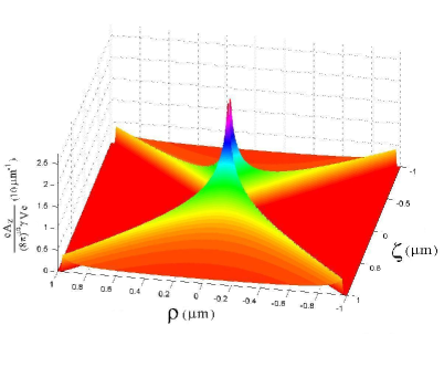
Figure 13: Behaviour of the field $\psi\equiv A_{z}$ generated by a charge supposed to be Superluminal, as a function of $\rho$ and $\zeta\equiv z-Vt$, evaluated for $\gamma=1$ (i.e., for $V=c\sqrt{2}$): According to ref.[13]  [Of course, we skipped the points at which $\psi$ must diverge: namely, the vertex and the cone surface].

For comparison, one may recall that the classic X-shaped solution[14] of the homogeneous wave-equation —which is shown, e.g., in Figs.8, 9, 12— has the form (with $a>0$):

$\displaystyle{X\;=\;{\frac{V}{\sqrt{(a-i\zeta)^{2}+\rho^{2}(V^{2}-1)}}}}\;.$ (26)

The second one of eqs.(25) includes expression (26), given by the spectral parameter[38, 82] $a=0$, which indeed corresponds to the non-homogeneous case [the not negligible fact that for $a=0$ these equations differ for an imaginary unit[54, 83] will be discussed elsewhere].

It is rather important, at this point, to notice that such a solution, eq.(25), does represent a wave existing only inside the (unlimited) double cone ${\cal C}$ generated by the rotation around the $z$-axis of the straight lines $\rho=\pm\gamma\zeta$:  This too is in full agreement with the predictions of the extended theory of SR.  For the explicit evaluation of the electromagnetic fields generated by the Superluminal charge (and of their boundary values and conditions) we confine ourselves here to merely quoting ref.[13].  Incidentally, the same results found by following the above procedure can be obtained by starting from the four-potential associated with a subluminal charge (e.g., an electric charge at rest), and then applying to it the suitable Superluminal Lorentz “transformation”.  One should also notice that this double cone does not have much to do with the Cherenkov cone[54, 80, 84]; and that a Superluminal charge travelling at constant speed, in the vacuum, does not lose energy: See, e.g., Fig.14 [which reproduces figure 27 at page 80 of ref.[54]].

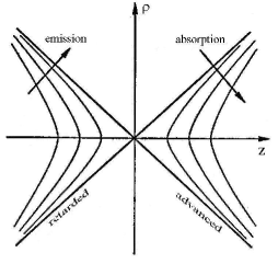
Figure 14: The spherical equipotential surfaces of the electrostatic field created by a charge at rest get transformed into two-sheeted rotation-hyperboloids, contained inside an unlimited double-cone, when the charge travels at Superluminal speed (cf. refs.[13, 54]). This figures shows, among the others, that a Superluminal charge travelling at constant speed, in a homogeneous medium like the vacuum, does not lose energy[80].  Let us mention, incidentally, that this double cone has nothing to do with the Cherenkov cone[84].  [The present picture is a reproduction of figure 27, appeared in 1986 at page 80 of ref.[54]].

Outside the cone ${\cal C}$, i.e., for $0<\gamma\mid{\zeta}\mid<\rho$, we get as expected no field, so that one meets a field discontinuity when crossing the double-cone surface. Nevertheless, the boundary conditions imposed by Maxwell equations are satisfied by our solution (25), since at each point of the cone surface the electric and the magnetic field are both tangent to the cone: also for a discussion of this point we refer to quotation[13].

Here, let us stress that, when $V\rightarrow\infty$, and therefore $\gamma\rightarrow 0$, the electric field tends to vanish, while the magnetic field tends to the value $H_{\phi}=-\pi e/\rho^{2}$: This does agree once more with what expected from extended SR, which predicted Superluminal charges to behave (in a sense) as magnetic monopoles. In the present paper we can only mention such a circumstance, and refer to citations[77, 54, 78, 83], and papers quoted therein.

5 APPENDIX: A Glance at the Experimental State-of-the-Art

Extended relativity can allow a better understanding of many aspects also of ordinary physics[54], even if Superluminal objects (tachyons) did not exist in our cosmos as asymptotically free objects.  Anyway, at least three or four different experimental sectors of physics seem to suggest the possible existence of faster-than-light motions, or, at least, of Superluminal group-velocities.  We are going to put forth in the following some information about the experimental results obtained in two of those different physics sectors, with a mere mention of the others.

Neutrinos – First: A long series of experiments, started in 1971, seems to show that the square ${m_{0}}^{2}$ of the mass $m_{0}$ of muon-neutrinos, and more recently of electron-neutrinos too, is negative; which, if confirmed, would mean that (when using a naïve language, commonly adopted) such neutrinos possess an “imaginary mass” and are therefore tachyonic, or mainly tachyonic[85, 54, 86].  [In extended SR, however, the dispersion relation for a free Superluminal object does become  $\omega^{2}-\mbox{\boldmath$k$}^{2}=-\Omega^{2}$,  or  $E^{2}-\mbox{\boldmath$p$}^{2}=-m_{\rm o}^{2}$,  and there is no need at all, therefore, of imaginary masses].

Galactic Micro-quasars – Second: As to the apparent Superluminal expansions observed in the core of quasars[87] and, recently, in the so-called galactic micro-quasars[88], we shall not really deal with that problem, too far from the other topics of this paper; without mentioning that for those astronomical observations there exist also orthodox interpretations, based on ref.[89], that are still accepted by the majority of the astrophysicists.  For a theoretical discussion, see ref.[90]. Here, let us only emphasize that simple geometrical considerations in Minkowski space show that a single Superluminal source of light would appear[90, 54]:  (i) initially, in the “optical boom” phase (analogous to the acoustic “boom” produced by an airplane travelling with constant supersonic speed), as an intense source which suddenly comes into view; and which, afterwards,  (ii) seems to split into TWO objects receding one from the other with speed  $V>2c$ [all this being similar to what has been actually observed, according to refs.[88]].

Evanescent waves and “tunnelling photons” – Third: Within quantum mechanics (and precisely in the tunnelling processes), it had been shown that the tunnelling time —firstly evaluated as a simple Wigner’s “phase time” and later on calculated through the analysis of the wavepacket behaviour— does not depend[91, 92] on the barrier width in the case of opaque barriers (“Hartman effect”). This implies Superluminal and arbitrarily large group-velocities $V$ inside long enough barriers: see Fig.15.

Figure 15: Behaviour of the average “penetration time” (in seconds) spent by a tunnelling wavepacket, as a function of the penetration depth (in ångstroms) down a potential barrier (from Olkhovsky et al., ref.[92]).  According to the predictions of quantum mechanics, the wavepacket speed inside the barrier increases in an unlimited way for opaque barriers; and the total tunnelling time does not depend on the barrier width.[91, 92]

Experiments that may verify this prediction by, say, electrons or neutrons are difficult and rare[93, 94]. Luckily enough, however, the Schroedinger equation in the presence of a potential barrier is mathematically identical to the Helmholtz equation for an electromagnetic wave propagating, for instance, down a metallic waveguide (along the $z$-axis): as shown, e.g., in refs.[95];  and a barrier height $U$ bigger than the electron energy $E$ corresponds (for a given wave frequency) to a waveguide of transverse size lower than a cut-off value. A segment of “undersized” guide —to go on with our example— does therefore behave as a barrier for the wave (photonic barrier), as well as any other photonic band-gap filters.  The wave assumes therein —like a particle inside a quantum barrier— an imaginary momentum or wavenumber and, as a consequence, results exponentially damped along $x$ [see, e.g. Fig.16]: It becomes an evanescent wave (going back to normal propagation, even if with reduced amplitude, when the narrowing ends and the guide returns to its initial transverse size).  Thus, a tunnelling experiment can be simulated by having recourse to evanescent waves (for which the concept of group velocity can be properly extended: see the first one of refs.[57]).

Figure 16: Picture of the damping taking place inside a barrier (from ref.[57]): this damping does reduce the amplitude of the tunnelling wavepacket, imposing a practical limit on the adoptable barrier length.

The fact that evanescent waves travel with Superluminal speeds (cf., e.g., Fig.17) has been actually verified in a series of famous experiments. Namely, various experiments, performed since 1992 onwards by G.Nimtz et al. in Cologne[96], by R.Chiao, P.G.Kwiat and A.Steinberg at Berkeley[97], by A.Ranfagni and colleagues in Florence[18], and by others in Vienna, Orsay, Rennes, etcetera[98], verified that “tunnelling photons” travel with Superluminal group velocities [Such experiments raised a great deal of interest[99], also within the non-specialized press, and were reported in Scientific American, Nature, New Scientist, etc.].  Let us further remark that also extended SR had predicted[100] evanescent waves to be endowed with faster-than-$c$ speeds; the whole matter appears to be therefore theoretically selfconsistent.  The debate in the current literature does not refer to the experimental results (which can be correctly reproduced even by numerical simulations[63, 64] based on Maxwell equations only: Cf. Figs.18,19), but rather to the question whether they allow, or do not allow, sending signals or information with Superluminal speed (see, e.g., refs.[101]).

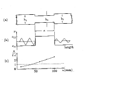
Figure 17: Simulation of tunnelling by experiments with evanescent classical waves (see the text), which were predicted to be Superluminal also on the basis of extended SR[100]. The figure shows one of the measurement results by Nimtz et al.[96]; that is, the average beam speed while crossing the evanescent region ( = segment of undersized waveguide, or “barrier”) as a function of its length. As theoretically predicted[91, 100], such an average speed exceeds $c$ for long enough “barriers”.  Further results appeared in ref.[102], and are reported below: see Figs.20 and 21 in the following .

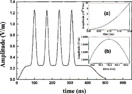
Figure 18: The delay of a wavepacket crossing a barrier (cf., e.g., Fig.17 is due to the initial discontinuity. We then performed suitable numerical simulations[63] by considering an (indefinite) undersized waveguide, and therefore eliminating any geometric discontinuity in its cross-section.  This figure shows the envelope of the initial signal.  Inset (a) depicts in detail the initial part of this signal as a function of time, while inset (b) depicts the gaussian pulse peak centered at $t=100$ ns .

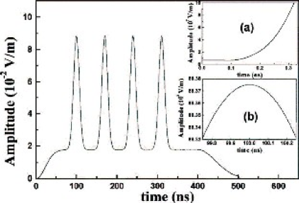
Figure 19: Envelope of the signal in the previous figure (Fig.18) after having travelled a distance $L=32.96$ mm through the mentioned undersized waveguide.  Inset (a) shows in detail the initial part (in time) of such arriving signal, while inset (b) shows the peak of the gaussian pulse that had been initially modulated by centering it at $t=100$ ns.  One can see that its propagation took zero time, so that the signal travelled with infinite speed.  The numerical simulation has been based on Maxwell equations only.  Going on from Fig.18 to Fig.19 one verifies that the signal strongly lowered its amplitute: However, the width of each peak did not change (and this might have some relevance when thinking of a Morse alphabet “transmission”: see the text) .

In the above-mentioned experiments one meets a substantial attenuation of the considered pulses —cf. Fig.16— during tunnelling (or during propagation in an absorbing medium): However, by employing “gain doublets”, it has been recently reported the observation of undistorted pulses propagating with Superluminal group-velocity with a small change in amplitude (see, e.g., ref.[103]).

Let us emphasize that some of the most interesting experiments of this series seem to be the ones with TWO or more “barriers” (e.g., with two gratings in an optical fiber[102], or with two segments of undersized waveguide separated by a piece of normal-sized waveguide[104]: Fig.20).

Figure 20: Very interesting experiments have been performed with TWO successive barriers, i.e., with two evanescence regions: For example, with two gratings in an optical fiber.  This figure[57] refers to the interesting experiment[104] performed with microwaves travelling along a metallic waveguide: the waveguide being endowed with two classical barriers (undersized guide segments). See the text .

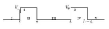
Figure 21: Scheme of the (non-resonant) tunnelling process, through two successive (opaque) quantum barriers. Far from resonances, the (total) phase time for tunnelling through the two potential barriers does depend neither on the barrier widths nor on the distance between the barriers (“generalized Hartman effect”)[105, 93, 106].  See the text.

For suitable frequency bands —namely, for “tunnelling” far from resonances—, it was found by us that the total crossing time does not depend on the length of the intermediate (normal) guide: that is, that the beam speed along it is infinite[105, 104, 93].  This does agree with what predicted by Quantum Mechanics for the non-resonant tunnelling through two successive opaque barriers[105]: Fig.21.  Such a prediction has been verified first theoretically, by Y.Aharonov et al.[105], and then, a second time, experimentally: by taking advantage of the circumstance that evanescence regions can consist in a variety of photonic band-gap materials or gratings (from multilayer dielectric mirrors, or semiconductors, to photonic crystals). Indeed, the best experimental confirmation has come by having recourse to two gratings in an optical fiber[102]: see Figs.22 and 23; in particular, the rather peculiar (and quite interesting) results represented by the latter.

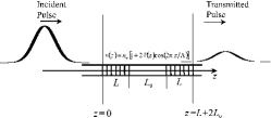
Figure 22: Realization of the quantum-theoretical set-up represented in Fig.21, by using, as classical (photonic) barriers, two gratings in an optical fiber[106].  The corresponding experiment has been performed by Longhi et al.[102]

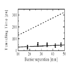
Figure 23: Off-resonance tunnelling time versus barrier separation for the rectangular symmetric DB FBG structure considered in ref.[102] (see Fig.22). The solid line is the theoretical prediction based on group delay calculations; the dots are the experimental points as obtained by time delay measurements [the dashed curve is the expected transit time from input to output planes for a pulse tuned far away from the stopband of the FBGs].  The experimental results[102] do confirm —as well as the early ones in refs.[104]]— the theoretical prediction of a “generalized Hartman Effect”: in particular, the independence of the total tunnelling time from the distance between the two barriers.

We cannot skip a further topic —which, being delicate, should not appear, probably, in a brief overview like this— since it is presently arising more and more interest[103].  Even if all the ordinary causal paradoxes seem to be solvable[58, 54, 57], nevertheless one has to bear in mind that (whenever it is met an object, ${\cal O}$, travelling with Superluminal speed) one may have to deal with negative contributions to the tunnelling times[107, 54, 93]: and this should not be regarded as unphysical. In fact, whenever an “object” (particle, electromagnetic pulse,,…) ${\cal O}$ overcomes[58, 54] the infinite speed with respect to a certain observer, it will afterwards appear to the same observer as the “anti-object” $\overline{{\cal O}}$ travelling in the opposite space direction[76, 54, 58].  For instance, when going on from the lab to a frame ${\cal F}$ moving in the same direction as the particles or waves entering the barrier region, the object ${\cal O}$ penetrating through the final part of the barrier (with almost infinite speed[92, 91, 63, 93], like in Figs.15) will appear in the frame ${\cal F}$ as an anti-object $\overline{{\cal O}}$ crossing that portion of the barrier in the opposite space-direction[58, 54, 76]. In the new frame ${\cal F}$, therefore, such anti-object $\overline{{\cal O}}$ would yield a negative contribution to the tunnelling time: which could even result, in total, to be negative.  For any clarifications, see the quoted references.  Let us stress, here, that even the appearance of such negative times had been predicted within SR itself[107], on the basis of its ordinary postulates; and has been recently confirmed by quantum-theoretical evaluations too[93, 108].  (In the case of a non-polarized beam,, the wave anti-packet coincides with the initial wave packet; if a photon is however endowed with helicity $\lambda=+1$, the anti-photon will bear the opposite helicity $\lambda=-1$).  From the theoretical point of view, besides the above-quoted papers (in particular refs.[93, 91]), see more specifically refs.[109].  On the (very interesting!) experimental side, see the intriguing papers [110].

Let us add here that, via quantum interference effects, it is possible to obtain dielectrics with refraction indices very rapidly varying as a function of frequency, also in three-level atomic systems, with almost complete absence of light absorption (i.e., with quantum induced transparency)[111].  The group velocity of a light pulse propagating in such a medium can decrease to very low values, either positive or negative, with no pulse distortion.  It is known that experiments have been performed both in atomic samples at room temperature, and in Bose-Einstein condensates, which showed the possibility of reducing the speed of light to a few meters per second.  Similar, but negative group velocities, implying a propagation with Superluminal speeds thousands of time higher than the previously mentioned ones, have been recently predicted also in the presence of such an “electromagnetically induced transparency”, for light moving in a rubidium condensate[112].  Finally, let us recall that faster-than-$c$ propagation of light pulses can be (and has been, in same cases) observed also by taking advantage of the anomalous dispersion near an absorbing line, or nonlinear and linear gain lines —as already seen—, or nondispersive dielectric media, or inverted two-level media, as well as of some parametric processes in nonlinear optics (cf., e.g., G.Kurizki et al.’s works).

D)  Superluminal Localized Solutions (SLS) to the wave equations. The “X-shaped waves” – The fourth sector (to leave aside the others) is not less important. It came into fashion again, when it was rediscovered in a series of remarkable works that any wave equation —to fix the ideas, let us think of the electromagnetic case— admit also solutions as much sub-luminal as Super-luminal (besides the luminal ones, having speed $c/n$).  Let us recall, indeed, that, starting from pioneering works as H.Bateman’s, it had slowly become known that all wave equations admit soliton-like (or rather wavelet-type) solutions with sub-luminal group velocities.  Subsequently, also Superluminal solutions started to be written down (in one case[35] just by the mere application of a Superluminal Lorentz “transformation”[54]).

As we know, a remarkable feature of some new solutions of these (which attracted much attention for their possible applications) is that they propagate as localized, non-diffracting pulses, also because of their self-reconstruction property.   It is easy to realize the practical importance, for instance, of a radio transmission carried out by localized beams, independently of their speed; but non-diffracting wave packets can be of use even in theoretical physics for a reasonable representation of elementary particles; and so on.  Incidentally, from the point of view of elementary particles, it can be a source of meditation the fact that the wave equations possess pulse-type solutions that, in the subluminal case, are ball-like (cf. Fig.24): this can have a bearing on the corpuscle/wave duality problem met in quantum physics (besides agreeing, e.g., with Fig.11). Further comments on this point are to be found below.

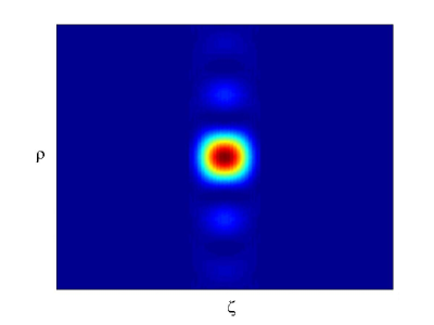
Figure 24: The wave equations possess pulse-type solutions that, in the subluminal case, are ball-like, in agreement with Fig.11.  For comments, see the text.

At the cost of repeating ourselves, let us emphasize once more that, within extended SR, since 1980 it had been found that —whilst the simplest subluminal object conceivable is a small sphere, or a point in the limiting case— the simplest Superluminal objects results by contrast to be (see refs.[9], and Figs.11 and 12 of this paper) an “X-shaped” wave, or a double cone as its limit, which moreover travels without deforming —i.e., rigidly— in a homogeneous medium.  It is not without meaning that the most interesting localized solutions to the wave equations happened to be just the Superluminal ones, and with a shape of that kind.  Even more, since from Maxwell equations under simple hypotheses one goes on to the usual scalar wave equation for each electric or magnetic field component, one expected the same solutions to exist also in the field of acoustic waves, of seismic waves, and of gravitational waves too: and this has already been demonstrated in the literature for all those cases, and especially in Acoustics.  Actually, such pulses (as suitable superpositions of Bessel beams) were mathematically constructed for the first time, by Lu et al. in Acoustics: and were then called “X-waves” or rather X-shaped waves.  (One should not forget that, however, LWs have been constructed in exact form even for other equations, as Schroedinger’s and as Einstein’s).

It is indeed important for us that the X-shaped waves have been really produced in experiments, both with acoustic and with electromagnetic waves; that is, X-pulses were produced that, in their medium, travel undistorted with a speed larger than sound, in the first case, and than light, in the second case.  In Acoustics, the first experiment was performed by Lu et al. themselves in 1992, at the Mayo Clinic (and their papers received the first IEEE 1992 award).  In the electromagnetic case, certainly more intriguing, Superluminal localized X-shaped solutions were first mathematically constructed (cf., e.g., Fig.25) in refs.[15], and later on experimentally produced by Saari et al.[17] in 1997

Figure 25: Real part of the Hertz potential and of the field components of the localized electromagnetic (“classic”, axially symmetric) X-shaped wave predicted, and first mathematically constructed for the electromagnetic case, in refs.[15].  For the meaning of the various panels, see the quoted references.  The dimension of each panel is 4 m (in the radial direction) ${\times}$ 2 mm (in the propagation direction).  [The values shown on the right-top corner of each panel represent the maxima and the minima of the images before normalization for display (MKSA units)] .

at Tartu by visible light (Fig.26), and more recently by Ranfagni et al. at Florence by microwaves[18].  In the theoretical sector the activity has been not less intense, in order to build up —for example— analogous new solutions with finite total energy or more suitable for high frequencies, on one hand, and localized solutions Superluminally propagating even along a normal waveguide (cf. Fig.27), on another hand, and so on.

Figure 26: Scheme of the experiment by Saari et al., who announced (PRL of 24 Nov.1997) the production in optics of the beams depicted in the previous Fig.25.   In the present figure one can see what it was shown by the experimental results: Namely, that the “X-shaped” waves are Superluminal: indeed, they, running after plane waves (the latter regularly travelling with speed $c$), do catch up with the considered plane waves.  An analogous experiment has been later on performed with microwaves at Florence by Ranfagni et al. (PRL of 22 May 2000).

Figure 27: In this figure a couple of elements are depicted of one of the trains of X-shaped pulses, mathematically constructed in ref.[113], which propagate down a coaxial guide (in the TM case): This picture is just taken from ref.[113],  but analogous X-pulses exist (with infinite or finite total energy) for propagation along a cylindrical, normal-sized metallic waveguide].

Let us eventually recall the problem of producing an X-shaped Superluminal wave like the one in Fig.12, but truncated —of course– in space and in time (by use of a finite antenna, radiating for a finite time): in such a situation, the wave is known to keep its localization and Superluminality only till a certain depth of field [i.e., as long as they are fed by the waves arriving (with speed $c$) from the antenna], decaying abruptly afterwards.[36, 38]  Let us add that various authors, taking account, e.g., of the time needed for fostering such Superluminal waves, have concluded that these localized Superluminal pulses are unable to transmit information faster than $c$.  Many of these questions have been discussed in what precedes; for further details, see the second of refs.[15].

Anyway, the existence of the X-shaped Superluminal (or Super-sonic) pulses seem to constitute, together, e.g., with the Superluminality of evanescent waves, a confirmation of extended SR: a theory[54] based on the ordinary postulates of SR and that consequently does not appear to violate any of the fundamental principles of physics.  It is curious moreover, that one of the first applications of such X-waves (that takes advantage of their propagation without deformation) has been accomplished in the field of medicine, and precisely —as we know— of ultrasound scanners[19, 20]; while the most important applications of the (subluminal!) Frozen Waves will very probably affect, once more, human health problems like the cancerous ones.

After the “digression” constituted by the above Appendix, let us go on to the Second Part of this work, with a slightly more technical[114] review about the physical and mathematical characteristics of the Localized Waves and about some interesting applications. [In the Third Part we shall deal with the ones endowed with zero speed, i.e., with a static envelope, and, more in general, with the subluminal LWs].

SECOND PART

STRUCTURE OF THE NONDIFFRACTING WAVES

AND SOME INTERESTING APPLICATIONS

6 Foreword

Since the early works[113-116] on the so-called nondiffracting waves (or “Localized Waves”), a great deal of results has been published on this important subject, from both the theoretical and the experimental point of view. Initially, the theory was developed taking into account only free space; however, in recent years, it has been extended for more complex media exhibiting effects such as dispersion[117-119], nonlinearity[122], anisotropy[123] and losses[124]. Such extensions have been carried out along with the development of efficient methods for obtaining nondiffracting beams and pulses in the subluminal, luminal and Superluminal regimes[123-130].

This Second Part addresses some theoretical methods related to nondiffracting solutions of the linear wave equation in unbounded homogeneous media, as well as to some interesting applications of such solutions.[114]

The usual cylindrical coordinates $(\rho,\phi,z)$ will be used here. We already know that in these coordinates the linear wave equation is written as

$$\frac{1}{\rho}\frac{\partial}{\partial\rho}\left(\rho\frac{\partial\Psi}{\partial\rho}\right)+\frac{1}{\rho^{2}}\frac{\partial^{2}\Psi}{\partial\phi^{2}}+\frac{\partial^{2}\Psi}{\partial z^{2}}-\frac{1}{c^{2}}\frac{\partial^{2}\Psi}{\partial t^{2}}\;=\;0$$ (27)

In Section VII we analyse the general structure of the Localized Waves, develop the so called Generalized Bidirectional Decomposition, and use it to obtain several luminal and Superluminal nondiffracting wave solutions of eq.(27).

In Section VIII we develop a kind of space-time focusing method by a continuous superposition of X-Shaped pulses of different velocities.

Section IX addresses the properties of chirped optical X-Shaped pulses propagating in material media without boundaries.

Subsequently, on the basis of what expounded in Section VII, we shall show at the beginning of the Third Part (in Section X) how a suitable superposition of Bessel beams can be even used to obtain stationary localized wave fields with high transverse localization, and whose longitudinal intensity pattern can assume any desired shape within a chosen interval $0\leq z\leq L$ of the propagation axis.

For containing the length of this review, we had, obviously, to skip many interesting results.  Let us just mention, for example, that rather simple analytic expressions, capable of describing the longitudinal (on-axis) evolution of axially-symmetric nondiffracting pulses, have been recently worked out in ref.[192] even for pulses truncated by finite apertures. By comparing what easily provided by such expressions, for several situations (involving subluminal, luminal, or Superluminal localized pulses), with the results obtained by numerical evaluations of the Rayleigh-Sommerfeld diffraction integrals, an exellent agreement has been found. Therefore, those new closed-form expressions dispense with the need of time-consuming numerical simulations (and provide an effective tool for finding out the most important properties of the truncated localized pulses).

7 Spectral structure of the Localized Waves and the Generalized Bidirectional Decomposition

An effective way to understand the concept of the (ideal) nondiffracting waves is furnishing a precise mathematical definition of these solutions, so to extract the necessary spectral structure from them.

Intuitively, an ideal nondiffracting wave (beam or pulse) can be defined as a wave capable of maintaining indefinitely its spatial form (apart from local variations) while propagating.

We can express such a characteristic by saying that a localized wave has to possess the property[124,125]

$$\Psi(\rho,\phi,z,t)\;=\;\Psi(\rho,\phi,z+\Delta z_{0},t+\frac{\Delta z_{0}}{V})$$ (28)

where $\Delta z_{0}$ is a certain length and $V$ is the pulse propagation speed that here can assume any value: $0\leq V\leq\infty$.

In terms of a Fourier Bessel expansion, we can write a function $\Psi(\rho,\phi,z,t)$ as

$$\Psi(\rho,\phi,z,t)\;=\;\sum_{n=-\infty}^{\infty}\left[\int_{0}^{\infty}{\rm d}k_{\rho}\,\int_{-\infty}^{\infty}{\rm d}k_{z}\,\int_{-\infty}^{\infty}{\rm d}\omega\,k_{\rho}A_{n}^{{}^{\prime}}(k_{\rho},k_{z},\omega)J_{n}(k_{\rho}\rho)e^{ik_{z}z}e^{-i\omega t}e^{in\phi}\right]\,.$$ (29)

On using the translation property of the Fourier transforms $\emph{T}[f(x+a)]={\rm exp}(ika)\emph{T}[f(x)]$, we have that $A_{n}^{{}^{\prime}}(k_{\rho},k_{z},\omega)$ and ${\rm exp}[i(k_{z}\Delta z_{0}-\omega\Delta z_{0}/V)]A_{n}^{{}^{\prime}}(k_{\rho},k_{z},\omega)$ are the Fourier Bessel transforms of the l.h.s and r.h.s. functions in eq.(28). And from this same equation we can get[124,125] the fundamental constraint linking the angular frequency $\omega$ and the longitudinal wavenumber $k_{z}$:

$$\omega\;=\;Vk_{z}+2m\pi\frac{V}{\Delta z_{0}}$$ (30)

with $m$ an integer. Obviously, this constraint can be satisfied by means of the spectral functions $A_{n}^{{}^{\prime}}(k_{\rho},k_{z},\omega)$.

Now, let us explicitly mention that constraint (30) does not imply any breakdown of the wave equation. In fact, when inserting expression (29) in the wave equation (27), one gets that

$$\frac{\omega^{2}}{c^{2}}\;=\;k_{z}^{2}+k_{\rho}^{2}\;.$$ (31)

So, to obtain a solution of the wave equation by (29), the spectrum $A_{n}^{{}^{\prime}}(k_{\rho},k_{z},\omega)$ must possess the form

$$A_{n}^{{}^{\prime}}(k_{\rho},k_{z},\omega)\;=\;A_{n}(k_{z},\omega)\,\delta\left[k_{\rho}^{2}-\left(\frac{\omega^{2}}{c^{2}}-k_{z}^{2}\right)\right]$$ (32)

where $\delta(.)$ is the Dirac delta function. With this, we can write a solution of the wave equation as

$$\Psi(\rho,\phi,z,t)\;=\;\sum_{n=-\infty}^{\infty}\left[\int_{0}^{\infty}{\rm d}\omega\,\int_{-\omega/c}^{\omega/c}{\rm d}k_{z}A_{n}(k_{z},\omega)J_{n}\left(\rho\sqrt{\frac{\omega^{2}}{c^{2}}-k_{z}^{2}}\right)e^{ik_{z}z}e^{-i\omega t}e^{in\phi}\right]$$ (33)

where we have considered positive angular frequencies only.

Equation (33) is a superposition of Bessel beams and it is understood that the integrations in the $(\omega,k_{z})$ plane are confined to the region $0\leq\omega\leq\infty$ and $-\omega/c\leq k_{z}\leq\omega/c\,$.

Now, to obtain an ideal nondiffracting wave, the spectra $A_{n}(k_{z},\omega)$ must obey the fundamental constraint (30), and so we write

$$A_{n}(k_{z},\omega)\;=\;\sum_{m=-\infty}^{\infty}\,S_{nm}(\omega)\delta\left[\omega-(Vk_{z}+b_{m})\right]$$ (34)

where $b_{m}$ are constants representing the terms $2m\pi V/\Delta z_{0}$ in eq.(30), and $S_{nm}(\omega)$ are arbitrary frequency spectra.

By inserting eq.(34) into eq.(33), we get a general integral form of the ideal nondiffracting wave (28):

$$\Psi(\rho,\phi,z,t)\;=\;\sum_{n=-\infty}^{\infty}\,\sum_{m=-\infty}^{\infty}\psi_{nm}(\rho,\phi,z,t)$$ (35)

with

$$\begin{array}[]{clcr}\psi_{nm}(\rho,\phi,z,t)\;=&\displaystyle{e^{-ib_{m}z/V}\,\int_{(\omega_{{\rm min}})_{m}}^{(\omega_{{\rm max}})_{m}}\,d\omega\,S_{nm}(\omega)}\\ \\ &\times\displaystyle{J_{n}\left(\rho\sqrt{\left(\frac{1}{c^{2}}-\frac{1}{V^{2}}\right)\omega^{2}+\frac{2b}{V^{2}}\omega-\frac{b^{2}}{V^{2}}}\right)e^{i\frac{\omega}{V}(z-Vt)}e^{in\phi}}\end{array}$$ (36)

where $\omega_{{\rm min}}$ and $\omega_{{\rm max}}$ depend on the values of V:

• for subluminal $(V<c)$ localized waves: $b_{m}>0$, $(\omega_{{\rm min}})_{m}=cb_{m}/(c+V)$ and $(\omega_{{\rm max}})_{m}=cb_{m}/(c-V)$;

• for luminal $(V=c)$ localized waves: $b_{m}>0$, $(\omega_{{\rm min}})_{m}=b_{m}/2$ and $(\omega_{{\rm max}})_{m}=\infty$;

• for Superluminal $(V>c)$ localized waves: $b_{m}\geq 0$, $(\omega_{{\rm min}})_{m}=cb_{m}/(c+V)$ and $(\omega_{{\rm max}})_{m}=\infty$. Or $b_{m}<0$, $(\omega_{{\rm min}})_{m}=cb_{m}/(c-V)$ and $(\omega_{{\rm max}})_{m}=\infty$.

It is important to notice that each $\psi_{nm}(\rho,\phi,z,t)$ in the superposition (35) is a truly nondiffracting wave (beam or pulse) and the superposition of them, (35), is just the most general form to represent a nondiffracting wave defined by eq.(28). Due to this fact, the search for methods capable of providing analytic solutions for $\psi_{nm}(\rho,\phi,z,t)$, eq.(36), becomes an important task.

Let us recall that equation (36) is also a Bessel beam superposition, but with constraint (30) linking their angular frequencies and longitudinal wavenumbers.

In spite of the fact that expression (36) represents ideal nondiffracting waves, it is difficult to obtain closed analytic solutions from it. Due to this, we are going to develop a method capable of overcoming such a difficulty, providing several interesting localized wave solutions (luminal and Superluminal) of arbitrary frequencies, including some solutions endowed with finite energy.

7.1 The Generalized Bidirectional Decomposition

For reasons that will be clear soon, instead of dealing with the integral expression (35), our starting point is the general expression (33).  Here, for simplicity, we shall restrict ourselves to axially symmetric solutions, adopting the spectral functions

$$A_{n}(k_{z},\omega)\;=\;\delta_{n0}A(k_{z},\omega)$$ (37)

where $\delta_{n0}$ is the Kronecker delta.

In this way, we get the following general solution (considering positive angular frequencies only), which describes axially symmetric waves:

$$\Psi(\rho,\phi,z,t)\;=\;\int_{0}^{\infty}{\rm d}\omega\,\int_{-\omega/c}^{\omega/c}{\rm d}k_{z}A(k_{z},\omega)J_{0}\left(\rho\sqrt{\frac{\omega^{2}}{c^{2}}-k_{z}^{2}}\right)e^{ik_{z}z}e^{-i\omega t}$$ (38)

As we have seen, we can obtain ideal nondiffracting waves, given that the spectrum $A(k_{z},\omega)$ satisfies the linear relationship (30). Therefore, it becomes natural to choose new spectral parameters, in place of $(\omega,k_{z})$, that make easier to implement the mentioned constraint[124,125].  With this in mind, let us choose the new spectral parameters $(\alpha,\beta)$

$$\alpha\equiv\frac{1}{2V}(\omega+Vk_{z})\;;\;\;\;\beta\equiv\frac{1}{2V}(\omega-Vk_{z})\;.$$ (39)

Let us consider here only luminal $(V=c)$ and Superluminal $(V>c)$ nondiffracting pulses.

With the change of variables (39) in the integral solution(38), and considering $(V\geq c)$, the integration limits on $\alpha$ and $\beta$ have to satisfy the three inequalities

$$\left\{\begin{array}[]{clcr}0<\alpha+\beta<\infty\\ \\ \alpha\geq\displaystyle{\frac{c-V}{c+V}}\beta\\ \\ \alpha\geq\displaystyle{\frac{c+V}{c-V}}\beta\end{array}\right.$$ (40)

Let us suppose both $\alpha$ and $\beta$ to be positive $[\alpha,\,\beta\geq 0]$. The first inequality in (40) is then satisfied; while the coefficients $(c-V)/(c+V)$ and $(c+V)/(c-V)$ entering relations (40) are both negatives (since $V\geq c$). As a consequence, the other two inequalities in (40) result to be automatically satisfied. In other words, the integration limits $0\leq\alpha\leq\infty$ and $0\leq\beta\leq\infty$ are contained” into the limits (40) and are therefore acceptable. Indeed, they constitute a rather suitable choice for facilitating all the subsequent integrations.

Therefore, instead of eq.(38), we shall consider the (more easily integrable) Bessel beam superposition in the new variables [with $V\geq c$]

$$\Psi(\rho,\zeta,\eta)=\int_{0}^{\infty}{\rm d}\alpha\int_{0}^{\infty}{\rm d}\beta A(\alpha,\beta)\,J_{0}\left(\rho\,\sqrt{\left(\frac{V^{2}}{c^{2}}-1\right)(\alpha^{2}+\beta^{2})+2\left(\frac{V^{2}}{c^{2}}+1\right)\alpha\beta}\right)e^{i\alpha\zeta}e^{-i\beta\eta}$$ (41)

where we have defined

$$\zeta\equiv z-Vt\;;\;\;\;\;\;\;\;\eta\equiv z+Vt\;.$$ (42)

The present procedure is a generalization of the so-called “bidirectional decomposition” technique[125], which was devised in the past for $V=c$.

From the new spectral parameters defined in transformation (39), it is easy to see that the constraint (30), i.e. $\omega=Vk_{z}+b$, is implemented just by making

$$A(k_{z},\omega)\rightarrow A(\alpha,\beta)\;=\;S(\alpha)\delta(\beta-\beta_{0})$$ (43)

with $\beta_{0}=b/2V$. The delta function $\delta(\beta-\beta_{0})$ in the spectrum (43) means that we are integrating Bessel beams along the continuous line $\omega=Vk_{z}+2V\beta_{0}$ and, in this way, the function $S(\alpha)$ will give the frequency dependence of the spectrum: $S(\alpha)\rightarrow S(\omega/V-\beta_{0})$.

This method constitutes a simple, natural way for obtaining pulses with field concentration on $\rho=0$ and at $\zeta=0\rightarrow z=Vt$.

Now, it is important to emphasize[127] that, when $\beta_{0}>0$ in (43), superposition (41) gets contributions from both backward and forward travelling Bessel beams, corresponding to the frequency intervals $V\beta_{0}\leq\omega<2V\beta_{0}$ (where $k_{z}<0$) and $2V\beta_{0}\leq\omega\leq\infty$ (where $k_{z}\geq 0$), respectively.  Nevertheless, we can obtain physical solutions when rendering the contribution of the backward-travelling components negligible, by choosing suitable weight functions $S(\alpha)$.

It is also worth noticing that we adopted the new spectral parameters $\alpha$ and $\beta$ just to obtain (closed-form) analytic localized wave solutions: The spectral characteristics of these new solutions can be brought into evidence by using transformations (39) and writing the corresponding spectrum in terms of the usual $\omega$ and $k_{z}$ spectral parameters.

In the following, we consider some cases with $\beta_{0}=0$ and $\beta_{0}>0$.

7.1.1 Closed analytic expressions describing some ideal nondiffracting pulses

Let us first consider, in eq.(41), spectra of the type (43) with $\beta_{0}=0$:

$$A(\alpha,\beta)\;=\;aV\,\delta(\beta)e^{-aV\alpha}$$ (44)

$$A(\alpha,\beta)\;=\;aV\,\delta(\beta)J_{0}(2d\sqrt{\alpha})e^{-aV\alpha}$$ (45)

$$A(\alpha,\beta)\;=\;\delta(\beta)\frac{\sin(d\alpha)}{\alpha}e^{-aV\alpha}\;,$$ (46)

$a>0$ and $d$ being constants.

One can obtain from the above spectra the following Superluminal LW solutions, respectively:

— from spectrum (44), we can use the identity (6.611.1) in ref.[133], obtaining the well known ordinary X xave solution (also called X-shaped pulse)

$$\Psi(\rho,\zeta)\;\equiv\;X\;=\;\frac{aV}{\sqrt{(aV-i\zeta)^{2}+\left(\frac{V^{2}}{c^{2}}-1\right)\rho^{2}}}\;;$$ (47)

— by using spectrum (45) and the identity (6.6444) of ref.[133], one gets

$$\Psi(\rho,\zeta)\;=\;X\ J_{0}\left(\sqrt{\frac{V^{2}}{c^{2}}-1}\;\;(aV)^{-2}d^{2}X^{2}\rho\right){\rm exp}\left[-(aV-i\zeta)\,(aV)^{-2}d^{2}\,X^{2}\right]\;;$$ (48)

— the Superluminal nondiffracting pulse

$$\begin{array}[]{clcr}\Psi(\rho,\zeta)\;=\;\sin^{-1}\,\left[2\displaystyle{\frac{d}{aV}}\left(\displaystyle{\sqrt{X^{-2}+(d/aV)^{2}+2\rho d(aV)^{-2}\sqrt{V^{2}/c^{2}-1}}}\right.\right.\\ \\ +\left.\left.\displaystyle{\sqrt{X^{-2}+(d/aV)^{2}-2\rho d(aV)^{-2}\sqrt{V^{2}/c^{2}-1}}}\;\right)^{-1}\right]\end{array}$$ (49)

is obtained from spectrum (46) by using identity (6.752.1) of ref.[133] for $a>0$ and $d>0$.

From the previous discussion, we get to know that any solutions obtained from spectra of the type (43) with $\beta_{0}=0$ are free from noncausal (backward travelling) components.

In addition, when $\beta_{0}=0$, we can see that the pulsed solutions depend on $z$ and $t$ through $\zeta=z-Vt$ only, and so propagate rigidly, i.e. without distortion. Such pulses can be transversally localized only if $V>c$, because if $V=c$ the function $\Psi$ has to obey the Laplace equation on the transverse planes[124,125].

Many others Superluminal localized waves can be easily constructed[127] from the above solutions just by taking the derivatives (of any order) with respect to $\zeta$. It is also possible to show[127] that the new solutions, obtained in this way, have their spectra shifted towards higher frequencies.

Now, let us pass to consider, in eq.(41), a spectrum of the type (43) with $\beta_{0}>0$:

$$A(\alpha,\beta)\;=\;aV\delta(\beta-\beta_{0})\,e^{-aV\alpha}$$ (50)

with $a$ a positive constant.

As we have seen, the presence of the delta function, with the constant $\beta_{0}>0$, implies that we are integrating (summing) Bessel beams along the continuous line $\omega=Vk_{z}+2V\beta_{0}$. Now, the function $S(\alpha)=aV{\rm exp}(-aV\omega)$ entails that we are considering a frequency spectrum of the type $S(\omega)\propto{\rm exp}(-a\omega)$, and therefore with a bandwidth given by $\Delta\omega=1/a$.

Since $\beta_{0}>0$, the interval $V\beta_{0}\leq\omega<2V\beta_{0}$ (or, equivalently, in this case, $0\leq\alpha<\beta_{0}$), corresponds to backward Bessel beams, i.e., negative values of $k_{z}$. However, we can get physical solutions when making the contribution of this frequency interval negligible. In our case, this can be obtained by making $a\beta_{0}V<<1$, so that the exponential decay of the spectrum $S$ with respect to $\omega$ is very slow, and the contribution of the interval $\omega\geq 2V\beta_{0}$ (where $k_{z}\geq 0$) largely overruns the $V\beta_{0}\leq\omega<2V\beta_{0}$ (where $k_{z}<0$) contribution.

Incidentally, let us note that, once we ensure the causal behaviour of the pulse by making $aV\beta_{0}<<1$ in (50), we have that $\Delta\alpha=1/aV>>\beta_{0}$, and one can therefore simplify the argument of the Bessel function, in the integrand of superposition (41), by neglecting the term $(V^{2}/c^{2}-1)\beta_{0}^{2}$. With this, the superposition (41), with the spectrum (50), can be written as

$$\Psi(\rho,\zeta,\eta)\approx aVe^{-i\beta_{0}\eta}\int_{0}^{\infty}{\rm d}\alpha J_{0}\left(\rho\sqrt{\left(\frac{V^{2}}{c^{2}}-1\right)\alpha^{2}+2\left(\frac{V^{2}}{c^{2}}+1\right)\alpha\beta_{0}}\right)e^{i\alpha\zeta}e^{-aV\alpha}$$ (51)

Now, we can use identity (6.616.1) of ref.[133] and obtain the new localized Superluminal solution called[127] Superluminal Focus Wave Mode (SFWM):

$$\Psi_{\rm SFWM}(\rho,\zeta,\eta)\;=\;{\rm e}^{-i\beta_{0}\eta}\;X\;\displaystyle{\exp\left[\frac{\beta_{0}(V^{2}+c^{2})}{V^{2}-c^{2}}\,\left((aV-i\zeta)-a\,VX^{-1}\right)\right]}$$ (52)

where, as before, $X$ is the ordinary X-pulse (47). The center of the SFWM is located on $\rho=0$ and $\zeta=0\,$ (i.e. at $z=Vt$). The intensity, $|\Psi|^{2}$, of this pulse propagates rigidly, it being a function of $\rho$ and $\zeta$ only. However, the complex function $\Psi_{\rm SFWM}$ (i.e. its real and imaginary parts) propagate with local variations, recovering their whole three dimensional form after each space and time interval $\Delta z_{0}=\pi/\beta_{0}$ and $\Delta t_{0}=\pi/\beta_{0}V$.

The SFWM solution written above, for $V\longrightarrow c^{+}$ reduces to the well known Focus Wave Mode (FWM) solution[125], travelling with speed $c$:

$$\Psi_{\rm FWM}(\rho,\zeta,\eta)\;=\;ac\displaystyle{\frac{{\rm e}^{-i\beta_{0}\eta}}{ac-i\zeta}\;\exp\left[-\frac{\beta_{0}\rho^{2}}{ac-i\zeta}\right]}\ .$$ (53)

Let us also emphasize that, since $\beta_{0}>0$, spectrum (50) results to correspond to angular frequencies $\omega\geq V\beta_{0}$. Thus, our new solution can be used to construct also high frequency pulses.

7.1.2 Finite energy nondiffracting pulses

In this subsection, we shall show how to get finite energy localized wave pulses, that can propagate for long distances while maintaining their spatial resolution, i.e., that possess a large depth of field.

As we have seen, ideal nondiffracting waves can be constructed by superposing Bessel beams [cf. eq.(38) for cylindrical symmetry] with a spectrum $A(\omega,k_{z})$ that satisfies a linear relationship between $\omega$ and $k_{z}$. In the general bidirectional decomposition method, this can be obtained by using spectra of the type (43) in superposition (41).

Solutions of that type possess an infinity depth of field: however, they are endowed with infinite energy[123,125]. To overcome this problem, we can truncate an ideal nondiffracting wave by a finite aperture, and the resulting pulse will have finite energy and a finite field-depth. Even so, such field-depths may be very large when compared with those of ordinary waves.

The problem in the present case is that the resulting field has to be calculated by diffraction integrals (such as the well known Rayleigh-Sommerfeld formula) and, in general, a closed analytic formula for the resulting pulse cannot be obtained.

However, there is another way to construct localized pulses with finite energy[127]. Namely, by using spectra $A(\omega,k_{z})$ in eq.(38) whose domains are not restricted exactly to the straight line $\omega=Vk_{z}+b$, but are defined in the surroundings of that line, wherein the spectra should have their main values concentrated (in other words, any spectrum has to be well localized in the vicinity of that line).

Similarly, in terms of the generalized bidirectional decomposition given in eq.(41), finite energy nondiffracting wave pulses can be constructed by adopting spectral functions $A(\alpha,\beta)$ well localized in the vicinity of the line $\beta=\beta_{0}$, quantity $\beta_{0}$ being a constant.

To exemplify this method, let us consider the following spectrum

$$A(\alpha,\beta)\;=\;\left\{\begin{array}[]{clr}&a\,q\,V\,e^{-aV\alpha}e^{-q(\beta-\beta_{0})}&{\rm for}\ \beta\geq\beta_{0}\\ \\ &0&{\rm for}\ 0\leq\beta<\beta_{0}\end{array}\right.$$ (54)

in superposition (41), quantities $a$ and $q$ being free positive constants and $V$ the peak’s pulse velocity (here $V\geq c$).

It is easy to see that the above spectrum is zero in the region above the $\beta=\beta_{0}$ line, while it decays in the region below (as well as along) such a line. We can concentrate this spectrum on $\beta=\beta_{0}$ by choosing values of $q$ in such a way that $q\beta_{0}>>1$. The faster the spectrum decay takes place in the region below the $\beta=\beta_{0}$ line, the larger the field-depth of the corresponding pulse results to be.

Besides this, once we choose $q\beta_{0}>>1$ to obtain pulses with a large field-depth, we can also minimize the contribution of the noncausal (backward) components by choosing $aV\beta_{0}<<1$; analogously with what we did and obtained for the SFWM case.

Again in analogy with the SFWM case, when we choose $q\beta_{0}>>1$ (i.e., a long field-depth) and $aV\beta_{0}<<1$ (a minimal contribution of the backward components), one is allowed to simplify the argument of the Bessel function, in the integrand of superposition (41), by neglecting the term $(V^{2}/c^{2}-1)\beta_{0}^{2}$.

With the help of the observations above, one can write the superposition (41), with spectrum (54), as:

$$\begin{array}[]{clcr}\Psi(\rho,\zeta,\eta)\,\approx&a\,q\,V\displaystyle{\int_{\beta_{0}}^{\infty}{\rm d}\beta\,\int_{0}^{\infty}{\rm d}\alpha\,J_{0}\left(\rho\,\sqrt{\left(\frac{V^{2}}{c^{2}}-1\right)\alpha^{2}+2\left(\frac{V^{2}}{c^{2}}+1\right)\alpha\beta}\,\right)}\\ \\ &\times\,\displaystyle{e^{-i\beta\eta}e^{i\alpha\zeta}e^{-q(\beta-\beta_{0})}\,e^{-aV\alpha}}\end{array}$$ (55)

and, using identity (6.616.1) given in ref.[133], we get

$$\Psi(\rho,\zeta,\eta)\,\approx q\,X\int_{\beta_{0}}^{\infty}{\rm d}\beta\,\displaystyle{e^{-q(\beta-\beta_{0})}e^{-i\beta\eta}{\rm exp}\left[\beta\,\frac{V^{2}+c^{2}}{V^{2}-c^{2}}\left(aV-i\zeta-aVX^{-1}\right)\right]},$$ (56)

which can be viewed as a superposition of the SFWM pulses (see eq.(52)).

The above integration can be easily performed and results[127] in the so called Superluminal Modified Power Spectrum (SMPS) pulse:

$$\Psi_{\rm SMPS}(\rho,\zeta,\eta)\;=\;q\,X\,\frac{{\rm exp}[(Y-i\eta)\beta_{0}]}{q-(Y-i\eta)}$$ (57)

where $X$ is the ordinary X-pulse (47) and $Y$ is defined by

$$Y\ \equiv\ \displaystyle{\frac{V^{2}+c^{2}}{V^{2}-c^{2}}\;\left[(aV-i\zeta)-aVX^{-1}\right]}\;.$$ (58)

The SMPS pulse is a Superluminal localized wave, with field concentration around $\rho=0$ and $\zeta=0\,$ (i.e., $z=Vt$), and with finite total energy. We will show that the depth of field, $Z$, of this pulse is given by $Z_{\rm SMPS}=q/2$.

An interesting property of the SMPS pulse is related to its transverse width (the transverse spot size at the pulse center). It can be shown from eq.(57) that, for the cases where $aV<<1/\beta_{0}$ and $q\beta_{0}>>1$, i.e., for the cases considered by us, the transverse spot size, $\Delta\rho$, of the pulse center ($\zeta=0$) is determined by the exponential function in (57) and is given by

$$\Delta\rho\;=\;c\,\sqrt{\frac{aV}{\beta_{0}(V^{2}+c^{2})}+\frac{V^{2}-c^{2}}{4\beta_{0}^{2}(V^{2}+c^{2})^{2}}}\;,$$ (59)

which clearly does not depend on $z$, and so remains constant during its propagation. In other words, in spite of the fact that the SMPS pulse suffers an intensity decrease during propagation, it preserves its transverse spot size. This interesting characteristic is not met in ordinary pulses, like the gaussian ones, where the amplitude of the pulse decreases and the width increases by the same factor.

Figure 28 shows the intensity of a SMPS pulse, with $\beta_{0}=33\,{\rm m}^{-1}$, $V=1.01c$, $a=10^{-12}\,$s and $q=10^{5}\,$m, at two different moments, for $t=0$ and after $50\,$km of propagation, where, as one can see, the pulse becomes less intense (precisely, with half of its initial peak intensity).  In spite of the intensity decrease, the pulse maintains its transverse width, as one can see from the 2D plots in Fig.(28), which show the field intensities in the transverse sections at $z=0$ and $z=q/2=50$ km.

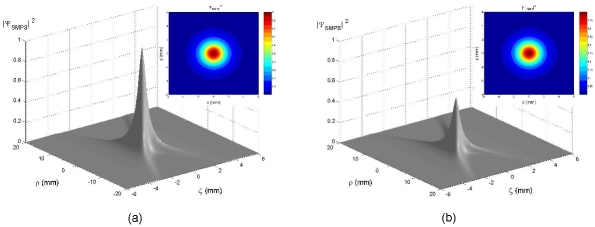
Figure 28: Representation of a Superluminal Modified Power Spectrum pulse, eq.(57).  Its total energy is finite (even without any truncation), and so it gets deformed while propagating, since its amplitude decreases with time.  In Fig.28a we represent, for $t=0$, the pulse corresponding to $\beta_{0}=33\,{\rm m}^{-1}$, $V=1.01c$, $a=10^{-12}\,$s and $q=10^{5}\,$m.  In Fig.28b it is depicted the same pulse after having travelled $50\;$km.

Other three important well known finite energy nondiffracting solutions can be obtained directly from the SMPS pulse:

— The first one, obtained from (57) by making $\beta_{0}=0$, is the so called[127] Superluminal Splash Pulse (SSP)

$$\Psi_{\rm SSP}(\rho,\zeta,\eta)\;=\;\frac{q\,X}{q+i\eta-Y}\;.$$ (60)

— The other two pulses are luminal. By taking the limit $V\rightarrow c^{+}$ in the SMPS pulse (57), we get the well known[125] luminal Modified Power Spectrum (MPS) pulse

$$\Psi_{\rm MPS}(\rho,\zeta,\eta)\;=\;\frac{a\,q\,c\,e^{-i\beta_{0}\eta}}{(q+i\eta)(ac-i\zeta)+\rho^{2}}\,{\rm exp}\left(\frac{-\beta_{0}\rho^{2}}{ac-i\zeta}\right)\;;$$ (61)

finally, by taking the limit $V\rightarrow c^{+}$ and making $\beta_{0}=0$ in the SMPS pulse [or, equivalently, by making $\beta_{0}=0$ in the MPS pulse (61), or,instead, by taking the limit $V\rightarrow c^{+}$ in the SSP (60)], we obtain the well known[125] luminal Splash Pulse (SP) solution

$$\Psi_{\rm SP}(\rho,\zeta,\eta)\;=\;\frac{a\,q\,c}{(q+i\eta)(ac-i\zeta)+\rho^{2}}\;.$$ (62)

It is also interesting to notice that the X and SFWM pulses can be obtained from the SSP and SMPS pulses (respectively) by making $q\rightarrow\infty$ in Eqs.(60) and (57). As a matter of fact, the solutions SSP and SMPS can be viewed as the finite energy versions of the X and SFWM pulses, respectively.

Some characteristics of the SMPS pulse:

Let us examine the on-axis ($\rho=0$) behaviour of the SMPS pulse.  On $\rho=0$ we have

$$\Psi_{\rm SMPS}(\rho=0,\zeta,\eta)\;=\;aqVe^{-i\beta_{0}z}[(aV-i\zeta)(q+i\eta)]^{-1}\;.$$ (63)

From this expression, we can show that the longitudinal localization $\Delta z$, for $t=0$, of the SMPS pulse square-magnitude is

$$\Delta z\;=\;2aV\;.$$ (64)

If we now define the field-depth $Z$ as the distance over which the pulse’s peak intensity is at least $50\%$ of its initial value, then we can obtain, from (63), the depth of field

$$Z_{\rm SMPS}\;=\;\frac{q}{2}\;,$$ (65)

which depends only on $q$, as we expected since $q$ regulates the concentration of the spectrum around the line $\omega=Vk_{z}+2V\beta_{0}$.

Now, let us examine the maximum amplitude $M$ of the real part of (63), which for $z=Vt$ writes ($\zeta=0$ and $\eta=2z$):

$$M_{\rm SMPS}\equiv{\rm Re}[\Psi_{\rm SMPS}(\rho=0,z=Vt)]\;=\;\frac{\cos(2\beta_{0}z)-2(z/q)\sin(2\beta_{0}z)}{1+4(z/q)^{2}}\;.$$ (66)

Initially, for $z=0$, $t=0$, one has $M=1$ and can also infer that:

(i) when $z/q<<1$, namely when $z<<Z$, equation (66) becomes

$$M_{\rm SMPS}\approx\cos(2\beta_{0}z)\;\;\;\;\;{\rm for}\;\;z<<Z$$ (67)

and the pulse’s peak actually oscillates harmonically with “wavelength” $\Delta z_{0}=\pi/\beta_{0}$ and “period” $\Delta t_{0}=\pi/V\beta_{0}$, all along its field-depth;

(ii) when $z/q>>1$, namely $z>>Z$, equation (66) becomes

$$M_{{\rm SMPS}}\approx-\frac{\sin(2\beta_{0}z)}{2z/q}\;\;\;\;{\rm for}\;\;z>>Z\;.$$ (68)

Therefore, beyond its depth of field, the pulse goes on oscillating with the same $\Delta z_{0}$, but its maximum amplitude decays proportionally to $z$.

In the next two Sections we are going to see applications of the localized wave pulses.

8 Space-Time Focusing of X-shaped Pulses

In this Section we are going to show how one can in general use any known Superluminal solution to obtain from it a large number of analytic expressions for space-time focused waves, endowed with a very strong intensity peak at the desired location. The method presented here is a natural extension of that developed by A.Shaarawi et al.[134], where the space-time focusing was achieved by superimposing a discrete number of ordinary X-waves, characterized by different values $\theta$ of the axicon angle.

In this Section, based on ref.[135], we shall go on to more efficient superpositions for varying velocities $V$, related to $\theta$ through the known[115,116,54] relation $V=c/\cos\theta$. This enhanced focusing scheme has the advantage of yielding analytic (closed-form) expressions for the spatio-temporally focused pulses.

Let us start by considering an axially symmetric ideal nondiffracting Superluminal wave pulse $\psi(\rho,z-Vt)$ in a dispersionless medium, where $V=c/\cos\theta>c$ is the pulse velocity, $\theta$ being the axicon angle. As we have seen in the previous Section, pulses like these can be obtained by a suitable frequency superposition of Bessel beams.  Suppose that we have now $N$ waves of the type $\psi_{n}(\rho,z-V_{n}(t-t_{n}))$, with different velocities $c<V_{1}<V_{2}<..<V_{N}$, and emitted at (different) times $t_{n}$; quantities $t_{n}$ being constants, while $n=1,2,...N$. The center of each pulse is located at $z=V_{n}(t-t_{n})$. To obtain a highly focused wave, we need all the wave components $\psi_{n}(\rho,z-V_{n}(t-t_{n}))$ to reach the given point, $z=z_{\rm f}$, at the same time $t=t_{\rm f}$. On choosing $t_{1}=0$ for the slowest pulse $\psi_{1}$, it is easily seen that the peak of this pulse reaches the point $z=z_{\rm f}$ at the time $t_{\rm f}=z_{\rm f}/V_{1}$. So we obtain that, for each $\psi_{n}$, the instant of emission $t_{n}$ must be

$$t_{n}\;=\;\left(\frac{1}{V_{1}}-\frac{1}{V_{n}}\right)z_{\rm f}\;.$$ (69)

With this in mind, we can construct other exact solutions to the wave equation, given by

$$\Psi(\rho,z,t)\;=\;\int_{V_{\rm min}}^{V_{\rm max}}\,{\rm d}V\,A(V)\,\psi\left(\rho,z-V\left(t-\left(\frac{1}{V_{\rm min}}-\frac{1}{V}\right)z_{\rm f}\right)\right)\ ,$$ (70)

where $V$ is the velocity of the wave $\psi(\rho,z-Vt)$ which enters the integrand of (70). While integrating, $V$ is considered as a continuous variable in the interval $[V_{\rm min},V_{\rm max}]$. In eq.(70), function $A(V)$ is the velocity distribution that specifies the contribution of each wave component (with velocity $V$) to the integration. The resulting wave $\Psi(\rho,z,t)$ can have a more or less strong amplitude peak at $z=z_{\rm f}$, at time $t_{\rm f}=z_{\rm f}/V_{\rm min}$, depending on $A(V)$ and on the difference $V_{\rm max}-V_{\rm min}$. Let us notice that also the resulting wavefield will propagate with a Superluminal peak velocity, depending on $A(V)$ too. In the cases when the velocity-distribution function is well concentrated around a certain velocity value, one can expect the wave (70) to increase its magnitude and spatial localization while propagating. Finally, the pulse peak acquires its maximum amplitude and localization at the chosen point $z=z_{\rm f}$, and at time $t=z_{\rm f}/V_{\rm min}$, as we know. Afterwards, the wave suffers a progressing spreading, and a decreasing of its amplitude.

8.1 Focusing Effects by Using Ordinary X-Waves

Here, we present a specific example by integrating (70) over the standard, classic[118] X-waves, $X=aV[(aV-i(z-Vt))^{2}+(V^{2}/c^{2}-1)\rho^{2}]^{-1/2}$. When using this ordinary X-wave, the largest spectral amplitudes are obtained for low frequencies. For this reason, one may expect that the solutions considered below will be suitable mainly for low frequency applications. Let us choose, then, the function $\psi$ in the integrand of eq.(70) to be $\psi(\rho,z,t)\equiv X(\rho,z-V(t-(1/V_{\rm min}-1/V)z_{\rm f}))$, viz.:

$$\psi(\rho,z,t)\equiv X\;=\;\displaystyle{\frac{aV}{\sqrt{\left[aV-i\left(z-V\left(t-\left(\frac{1}{V_{\rm min}}-\frac{1}{V}\right)z_{\rm f}\right)\right)\right]^{2}+\left(\frac{V^{2}}{c^{2}}-1\right)\rho^{2}}}}\;.$$ (71)

After some manipulations, one obtains the analytic integral solution

$$\Psi(\rho,z,t)\;=\;\int_{V_{\rm min}}^{V_{\rm max}}\,\displaystyle{\frac{aV\,A(V)}{\sqrt{PV^{2}+QV+R}}}{\rm d}V$$ (72)

with

$$\begin{array}[]{l}P\equiv\left[\left(a+i\left(t-\frac{z_{\rm f}}{V_{\rm min}}\right)\right)^{2}+\frac{\rho^{2}}{c^{2}}\right]\\ \\ Q\equiv 2\left(t-\frac{z_{\rm f}}{V_{\rm min}}-ai\right)(z-z_{\rm f})\\ \\ R\equiv\left[-(z-z_{\rm f})^{2}-\rho^{2}\right]\;.\end{array}$$ (73)

In what follows, we illustrate the behaviour of some new spatio-temporally focused pulses, by taking into consideration a few different velocity distributions $A(V)$. These new pulses are closed analytic exact solutions of the wave equation.

First example:

Let us consider our integral solution (72) with $A(V)=1\;{\rm s/m}$. In this case, the contribution of the X-waves is the same for all velocities in the allowed range $[V_{\rm min},V_{\rm max}]$.  On using identity 2.264.2 listed in ref.[133], we get the particular solution

$$\begin{array}[]{clcr}\Psi(\rho,z,t)\!\!&=\displaystyle{\frac{a}{P}}\,\displaystyle{\left(\sqrt{PV_{\rm max}^{2}+QV_{\rm max}+R}-\sqrt{PV_{\rm min}^{2}+QV_{\rm min}+R}\,\right)}\\ \\ &\;\;\;\displaystyle{+\frac{a\,Q}{2P^{3/2}}\,{\rm ln}\left(\frac{2\,\sqrt{P(PV_{\rm min}^{2}+QV_{\rm min}+R)}+2PV_{\rm min}+Q}{2\,\sqrt{P(PV_{\rm max}^{2}+QV_{\rm max}+R)}+2PV_{\rm max}+Q}\right)}\ ,\end{array}$$ (74)

where $P$, $Q$ and $R$ are given in eq.(73). A 3-dimensional (3D) plot of this function is provided in Fig.29; where we have chosen $a=10^{-12}$ s,  $V_{\rm min}=1.001\;c$,  $V_{\rm max}=1.005\;c$ and $z_{\rm f}=200\;$cm. It can be seen that this solution exhibits a rather evident space-time focusing. An initially spread-out pulse (shown for $t=0$) becomes highly localized at $t=t_{\rm f}=z_{\rm f}/V_{\rm min}=6.66\;$ns, the pulse peak amplitude at $z_{\rm f}$ being $40.82$ times greater than the initial one. In addition, at the focusing time $t_{\rm f}$ the field is much more localized than at any other times. The velocity of this pulse is approximately $V=1.003\;c$.

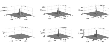
Figure 29: Space-time evolution of the Superluminal pulse represented by eq.(74); the chosen parameter values are $a=10^{-12}\;$s;  $V_{\rm min}=1.001\;c$;  $V_{\rm max}=1.005\;c$ while the focusing point is at $z_{\rm f}=200\;$cm.  One can see that this solution is associated with a rather good spatio-temporal focusing.  The field amplitude at $z=z_{\rm f}$ is 40.82 times larger than the initial one.  The field amplitude is normalized at the space-time point $\rho=0,\ z=z_{\rm f},\ t=t_{\rm f}$.

Second example:

In this case we choose $A(V)=1/V\;$s/m, and, using the identity 2.261 in ref.[133], eq.(72) yields

$$\Psi(\rho,z,t)\;=\;\displaystyle{\frac{a}{\sqrt{P}}\,{\rm ln}\left(\frac{2\,\sqrt{P(PV_{\rm max}^{2}+QV_{\rm max}+R)}+2PV_{\rm max}+Q}{2\,\sqrt{P(PV_{\rm min}^{2}+QV_{\rm min}+R)}+2PV_{\rm min}+Q}\right)}\ .$$ (75)

Other exact closed-form solutions can be obtained[135] by considering, for instance, velocity distributions like $A(V)=1/V^{2}$ and $A(V)=1/V^{3}$.

Once more, we can actually construct many others spatio-temporally focused pulses from the above solutions, just by taking their time derivatives (of any order). It is possible to show[135] that also the new solutions obtained in this way have their spectra shifted towards higher frequencies.

9 Chirped Optical X-Type Pulses in Material Media

The theory of the localized waves was initially developed for free space (vacuum). In 1996, Sõnajalg et al.[119] showed that the localized wave theory can be extended to include (unbounded) dispersive media. This was obtained by making the axicon angle of the Bessel beams (BBs) vary with the frequency[117-119] in such a way that a suitable frequency superposition of these beams does compensate for the material dispersion. Soon after this idea was reported, many interesting nondiffracting/nondispersive pulses were obtained theoretically[117-119] and experimentally[119].  In spite of such an extended method to be of remarkable importance, working well in theory, its experimental implementation is not so simple.

In 2004 Zamboni-Rached et al.[136] developed a simpler way to obtain pulses capable of recovering their spatial shape, both transversally and longitudinally, after some propagation. It consisted in using chirped optical X-typed pulses, while keeping the axicon angle fixed. Let us recall that, by contrast, chirped Gaussian pulses in unbounded material media may recover only their longitudinal shape, since they undergo a progressing transverse spreading while propagating.

The present Section is devoted to this approach.  Let us start with an axially-symmetric Bessel beam in a material medium with refractive index $n(\omega)$:

$$\psi(\rho,z,t)\;=\;J_{0}(k_{\rho}\rho)\,\exp(i\beta z)\,\exp(-i\omega t)\;,$$ (76)

where it must be obeyed the condition  $k_{\rho}^{2}=n^{2}(\omega)\omega^{2}/c^{2}-\beta^{2}$,  which connects among themselves the transverse and longitudinal wave numbers $k_{\rho}$ and $\beta$, and the angular frequency $\omega$. In addition, we impose that $k_{\rho}^{2}\geq 0$ and $\omega/\beta\geq 0$, to avoid a nonphysical behaviour of the Bessel function $J_{0}(.)$ and to confine ourselves to forward propagation only.  Once the conditions above are satisfied, we have the liberty of writing the longitudinal wave number as $\beta=(n(\omega)\omega\cos\theta)/c$ and, therefore, $k_{\rho}=(n(\omega)\omega\sin\theta)/c$; where (as in the free space case) $\theta$ is the axicon angle of the Bessel beam.

Now we can obtain an X-shaped pulse by performing a frequency superposition of these Bessel beams [BB], with $\beta$ and $k_{\rho}$ given by the previous relations:

$$\Psi(\rho,z,t)\;=\;\int_{-\infty}^{\infty}\,S(\omega)\,J_{0}\left(\frac{n(\omega)\omega}{c}\sin\theta\,\rho\right)\,\exp[i\beta(\omega)z]\,\exp(-i\omega t)\,{\rm d}\omega\;,$$ (77)

where $S(\omega)$ is the frequency spectrum, and the axicon angle is kept constant.  One can see that the phase velocity of each BB in our superposition (77) is different, and given by $V_{\rm phase}=c/(n(\omega)\cos\theta)$. So, the pulse represented by eq.(77) will suffer dispersion during its propagation.

As we said, the method developed by Sõnajalg et al.[119], and explored by others[118,119], to overcome this problem consisted in regarding the axicon angle $\theta$ as a function of the frequency, in order to obtain a linear relationship between $\beta$ and $\omega$.

Here, however, we choose to work with a fixed axicon angle, and we have to find out another way for avoiding dispersion and diffraction all along a certain propagation distance. To do that, we might choose a chirped gaussian spectrum $S(\omega)$ in eq.(77)

$$S(\omega)\;=\;\frac{T_{0}}{\sqrt{2\pi(1+iC)}}\,\,\exp[-q^{2}(\omega-\omega_{0})^{2}]\;\;\;\;{\rm with}\;\;\;\;\;q^{2}\;=\;\frac{T_{0}^{2}}{2(1+iC)}\;,$$ (78)

where $\omega_{0}$ is the central frequency of the spectrum, $T_{0}$ is a constant related with the initial temporal width, and $C$ is the chirp parameter (we chose as temporal width the half-width of the relevant gaussian curve when its heigth equals $1/e$ times its full heigth). Unfortunately, there is no analytic solution to eq.(77) with $S(\omega)$ given by eq.(78), so that some approximations are to be made.  Then, let us assume that the spectrum $S(\omega)$, in the surroundings of the carrier frequency $\omega_{0}$ , is narrow enough to guarantee that $\Delta\omega/\omega_{0}<<1$, so to ensure that $\beta(\omega)$ can be approximated by the first three terms of its Taylor expansion in the vicinity of $\omega_{0}$: That is,  $\beta(\omega)\approx\beta(\omega_{0})+\beta^{\prime}(\omega)|_{\omega_{0}}\,(\omega-\omega_{0})+(1/2)\beta^{\prime\prime}(\omega)|_{\omega_{0}}\,(\omega-\omega_{0})^{2}$;  when, after using $\beta=n(\omega)\omega\cos\theta/c$, it results that

$$\frac{\partial\beta}{\partial\omega}\;=\;\frac{\cos\theta}{c}\left[n(\omega)+\omega\,\frac{\partial n}{\partial\omega}\right]\,;\ \ \ \frac{\partial^{2}\beta}{\partial\omega^{2}}\;=\;\frac{\cos\theta}{c}\left[2\frac{\partial n}{\partial\omega}+\omega\frac{\partial^{2}n}{\partial\omega^{2}}\right]\;.$$ (79)

As we know, $\beta^{\prime}(\omega)$ is related to the pulse group-velocity by the relation $Vg=1/\beta^{\prime}(\omega)$. Here we can see the difference between the group-velocity of the X-type pulse (with a fixed axicon angle) and that of a standard gaussian pulse. Such a difference is due to the factor $\cos\theta$ in eq.(79). Because of it, the group-velocity of our X-type pulse is always greater than the gaussian’s. In other words, $(V_{\rm g})_{\rm X}=(1/\cos\theta)(V_{\rm g})_{{\rm gauss}}$.  We also know that the second derivative of $\beta(\omega)$ is related to the group-velocity dispersion (GVD) $\beta_{2}$ by $\beta_{2}=\beta^{\prime\prime}(\omega)$.  The GVD is responsible for the temporal (longitudinal) spreading of the pulse. Here one can see that the GVD of the X-type pulse is always smaller than that of the standard gaussian pulses, due the factor $\cos\theta$ in eq.(79). Namely: $(\beta_{2})_{\rm X}=\cos\theta(\beta_{2})_{\rm gauss}$.

On using the above results, we can write

$$\begin{array}[]{clcr}\Psi(\rho,z,t)\!\!&=\displaystyle{\frac{T_{0}\,\,\exp[i\beta(\omega_{0})z]\,\exp(-i\omega_{0}t)}{\sqrt{2\pi(1+iC)}}\,\int_{-\infty}^{\infty}{\rm d}\omega\,J_{0}\left(\frac{n(\omega)\omega}{c}\sin\theta\,\rho\right)}\\ \\ &\;\;\;\times\,\displaystyle{\exp\left\{i\frac{(\omega-\omega_{0})}{V_{\rm g}}\left[z-V_{\rm g}t\right]\right\}\,\exp\left\{(\omega-\omega_{0})^{2}\left[\frac{i\beta_{2}}{2}z-q^{2}\right]\right\}}\;.\end{array}$$ (80)

The integral in eq.(80) cannot be evaluated analytically, but for us it is sufficient to obtain the pulse behaviour. Let us analyse the pulse for $\rho=0$. In this case we get

$$\Psi(\rho=0,z,t)\;=\;\displaystyle{\frac{T_{0}\,\exp[i\beta(\omega_{0})z]\,\exp(-i\omega_{0}t)}{\sqrt{T_{0}^{2}-i\beta_{2}(1+iC)z}}\,\exp\left[\frac{-(z-V_{\rm g}t)^{2}(1+iC)}{2V_{\rm g}^{2}[T_{0}^{2}-i\beta_{2}(1+iC)z]}\right]}\;.$$ (81)

From eq.(81) one can immediately see that the initial temporal width of the pulse intensity is $T_{0}$ and that, after a propagation distance $z$, the time-width $T_{1}$ becomes

$$\frac{T_{1}}{T_{0}}\;=\;\left[\left(1+\frac{C\beta_{2}z}{T_{0}^{2}}\right)^{2}+\left(\frac{\beta_{2}z}{T_{0}^{2}}\right)^{2}\right]^{1/2}\;.$$ (82)

Relation (82) describes the pulse spreading-behaviour. One can easily show that such a behaviour depends on the sign (positive or negative) of the product $\beta_{2}C$, as is well known to happen for the standard gaussian pulses[137].  In the case $\beta_{2}C>0$, the pulse will monotonically become broader and broader with the distance $z$. On the other hand, if $\beta_{2}C<0$ the pulse will suffer, in a first stage, a narrowing, and then (during the rest of its propagation) it will spread . So, there will be a certain propagation distance AT after which the pulse will recover its initial temporal width ($T_{1}=T_{0}$). From relation (82), we can find such a distance $Z_{T1=T_{0}}$ (considering $\beta_{2}C<0$) to be

$$Z_{T_{1}=T_{0}}\;=\;\frac{-2CT_{0}^{2}}{\beta_{2}(C^{2}+1)}\;.$$ (83)

One may notice that the maximum distance at which our chirped pulse, with given $T_{0}$ and $\beta_{2}$, may recover its initial temporal width can be easily evaluated from eq.(83), and it results to be $L_{\rm disp}=T_{0}^{2}/\beta_{2}$. We shall call such a maximum value $L_{\rm disp}$ the “dispersion length”: It is the maximum distance the X-type pulse may travel while recovering its initial longitudinal shape. Obviously, if we want the pulse to reassume its longitudinal shape at some desired distance $z<L_{\rm disp}$, we have just to suitably choose a new value for the chirp parameter.

Let us emphasize that the property of recovering its own initial temporal (or longitudinal) width may be verified to exist also in the case of chirped standard gaussian pulses. However, the latter will suffer a progressing transverse spreading, which will not be reversible. The distance at which a gaussian pulse doubles its initial transverse width $w_{0}$  is  $z_{\rm diff}=\sqrt{3}\pi w_{0}^{2}/\lambda_{0}$, where $\lambda_{0}$ is the carrier wavelength. Thus, one can see that optical gaussian pulses with great transverse localization will get spoiled in a few centimeters or even less.

Now we shall show that it is possible to recover also the transverse shape of the chirped X-type pulse intensity; actually, it is possible to recover its entire spatial shape after a distance $Z_{T_{1}=T_{0}}$.  To see this, let us go back to our integral solution (80), and perform the change of coordinates  $(z,t)\rightarrow(\Delta z,t_{c}=z_{c}/V_{\rm g})$, with

$$\left\{\begin{array}[]{l}z\;=\;z_{c}+\Delta z\\ \\ \displaystyle{t=t_{c}\equiv\frac{z_{c}}{V_{\rm g}}}\end{array}\right.$$ (84)

where $z_{c}$ is the center of the pulse ($\Delta z$ is the distance from such a point), and $t_{c}$ is the time at which the pulse center is located at $z_{c}$. What we are going to do is comparing our integral solution (80), when $z_{c}=0$ (initial pulse), with that when $z_{c}=Z_{T_{1}=T_{0}}=-2CT_{0}^{2}/(\beta_{2}(C_{2}+1))$.  In this way, solution (80) can be written, when $z_{c}=0$, as

$$\begin{array}[]{clcr}\Psi(\rho,z_{c}=0,\Delta z)\!\!&=\displaystyle{\frac{T_{0}\,\,\,\exp(i\beta_{0}\Delta z)}{\sqrt{2\pi(1+iC)}}}\,\int_{-\infty}^{\infty}{\rm d}\omega\,J_{0}(k_{\rho}(\omega)\rho)\,\exp\left[\frac{-T_{0}^{2}\,(\omega-\omega_{0})^{2}}{2(1+C^{2})}\right]\\ \\ \\ &\;\;\;\displaystyle{\times\,\exp\left\{i\left[\frac{(\omega-\omega_{0})\Delta z}{V_{\rm g}}+\frac{(\omega-\omega_{0})^{2}\beta_{2}\Delta z}{2}+\frac{(\omega-\omega_{0})^{2}T_{0}^{2}C}{2(1+C^{2})}\right]\right\}}\\ \end{array}$$ (85)

where we have taken the value $q$ given by eq.(78).  To verify that the pulse intensity recovers its entire original form at $z_{c}=Z_{T_{1}=T_{0}}=-2\,CT_{0}^{2}/[\beta_{2}(C^{2}+1)]$, we can analyse our integral solution at that point, obtaining

$$\begin{array}[]{l}\Psi(\rho,z_{c}=Z_{T_{1}=T_{0}},\Delta z)\ =\ \displaystyle{\frac{T_{0}\,\,\displaystyle{\exp\left\{i\beta_{0}\left[z_{c}-\Delta z^{\prime}-\frac{cz_{c}}{\cos\theta\,n(\omega_{0})V_{\rm g}}\right]\right\}}}{\sqrt{2\pi(1+iC)}}}\\ \\ \\ \times\displaystyle{\int_{-\infty}^{\infty}}\displaystyle{{\rm d}\omega\,J_{0}(k_{\rho}(\omega)\rho)\,\exp\left[\frac{-T_{0}^{2}\,(\omega-\omega_{0})^{2}}{2(1+C^{2})}\right]}\\ \\ \\ \displaystyle{\times\,\exp\left\{-i\left[\frac{(\omega-\omega_{0})\Delta z^{\prime}}{V_{\rm g}}+\frac{(\omega-\omega_{0})^{2}\beta_{2}\Delta z^{\prime}}{2}+\frac{(\omega-\omega_{0})^{2}T_{0}^{2}C}{2(1+C^{2})}\right]\right\}}\\ \end{array}$$ (86)

where we put $\Delta z=-\Delta z^{\prime}$.  In this way, one immediately sees that

$$|\Psi(\rho,z_{c}=0,\Delta z)|^{2}=|\Psi(\rho,z_{c}=Z_{T_{1}=T_{0}},-\Delta z)|^{2}\;.$$ (87)

Therefore, from eq.(87) it is clear that the intensity of a chirped optical X-type pulse is able to recover its original three-dimensional shape, just with a longitudinal inversion at the pulse center. The present method results to be, therefore, a simple and effective procedure for compensating diffraction and dispersion in an unbounded material medium; and a method simpler than the one of varying the axicon angle with the frequency.

Let us stress again that one can determine the distance $z=Z_{T_{1}=T_{0}}\leq L_{\rm disp}$ at which the pulse takes on again its spatial shape by choosing a suitable value of the chirp parameter.

We have shown that the chirped X-type pulse recovers its three-dimensional shape after some distance, and we have also obtained an analytic description of the pulse longitudinal behaviour (for $\rho=0$) during propagation, by means of eq.(81). However, we have not got yet the same information about the pulse transverse behaviour: We just learned, till now, that it will be recovered at $z=Z_{T_{1}=T_{0}}$.

So, to complete the picture, we should find out also the transverse behaviour in the plane of the pulse center $z=V_{\rm g}t$:  We would then obtain quantitative information about the evolution of the pulse-shape during its entire propagation.  But we are not going to expound all the relevant mathematical details here; let us only state that the transverse behaviour of the pulse (in the plane $z=z_{c}=V_{\rm g}t$), during its whole propagation, can approximately be described by

$$\begin{array}[]{l}\Psi(\rho,z=z_{c},t=z_{c}/V_{\rm g})\,\approx\,\displaystyle{\frac{T_{0}\,\,\,\exp[i\beta(\omega_{0})z]\,\exp(-i\omega_{0}t)}{\sqrt{2\pi(1+iC)}}\,\,\frac{\exp\displaystyle{\left[\frac{-\tan^{2}\theta\,\rho^{2}}{8\,V_{\rm g}^{2}(-i\beta_{2}z_{c}/2\,+q^{2})}\right]}}{\sqrt{-i\beta_{2}z_{c}/2\,+q^{2}}}}\\ \\ \\ \times\,\displaystyle{\left[\Gamma(1/2)J_{0}\left(\frac{n(\omega_{0})\,\omega_{0}\,\sin\theta\,\rho}{c}\right)I_{0}\left(\frac{\tan^{2}\theta\,\rho^{2}}{8\,V_{\rm g}^{2}(-i\beta_{2}z_{c}/2\,+q^{2})}\right)\right.}\\ \\ \\ \left.+\displaystyle{2\sum_{p=1}^{\infty}\frac{2^{p}\Gamma(p+1/2)\Gamma(p+1)}{\Gamma(2p+1)}\,\,J_{2p}\left(\frac{n(\omega_{0})\,\omega_{0}\,\sin\theta\,\rho}{c}\right)I_{2p}\left(\frac{\tan^{2}\theta\,\rho^{2}}{8\,V_{\rm g}^{2}(-i\beta_{2}z_{c}/2\,+q^{2})}\right)}\right]\\ \end{array}$$ (88)

where $I_{p}(.)$ is the modified Bessel function of the first kind of order $p$, quantity $\Gamma(.)$ being the gamma function and $q$ being given by (78).  The interested reader can check ref.[136] for details on how eq.(LABEL:S4trans1) is obtained from eq.(80).

At a first sight, this solution appears to be very complicated, but the series in its r.h.s. gives a negligible contribution. This circumstance renders our solution (LABEL:S4trans1) of important practical interest, and we will use it in the following.  For additional information about the transverse pulse evolution (to be extracted from eq.(LABEL:S4trans1)), the reader can consult again ref.[136]. In the same paper, it is analysed how the generation by a finite aperture affects the chirped X-type pulses.

The valuable methods developed in ref.[136], and that we are partially revisiting in this Section, are of general interest, and work is in progress for applying them, e.g., also to the (different) case of the Schroedinger equation.

9.1 An example: Chirped Optical X-typed pulse in bulk fused Silica

For a bulk fused Silica, the refractive index $n(\omega)$ can be approximated by the Sellmeier equation[137]

$$n^{2}(\omega)\;=\;\displaystyle{1\,+\,\sum_{j=1}^{N}\,\frac{B_{j}\,\omega_{j}^{2}}{\omega_{j}^{2}-\omega^{2}}}\;,$$ (89)

where $\omega_{j}$ are the resonance frequencies, $B_{j}$ the strength of the $j$-th resonance, and $N$ the total number of the material resonances that appear in the frequency range of interest. For our purposes it is appropriate to choose $N=3$, which yields, for bulk fused silica[137], the values  $B_{1}=0.6961663$;  $B_{2}=0.4079426$;  $B_{3}=0.8974794$;  $\lambda_{1}=0.0684043\;\mu\;$m;  $\lambda_{2}=0.1162414\;\mu\;$m;  and $\lambda_{3}=9.896161\;\mu\;$m.

Now, let us consider in this medium a chirped X-type pulse, with $\lambda_{0}=0.2\,\mu$m,  $T_{0}=0.4\;$ps,  $C=-1$, and with axicon angle $\theta=0.00084\;$rad: That correspond to an initial central spot with $\Delta\rho_{0}=0.117\;$mm.  We get from eqs. (81) and (LABEL:S4trans1) the longitudinal and transverse pulse evolution, which are represented in Fig.30.

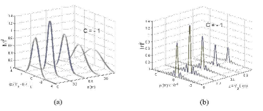
Figure 30: (a): Longitudinal-shape evolution of a chirped X-type pulse, propagating in fused silica with $\lambda_{0}=0.2\mu\;$m,  $T_{0}=0.4\;$ps,  $C=-1$, and axicon angle $\theta=0.00084\;$rad, which correspond to an initial transverse width of $\Delta\rho_{0}=0.117\;$mm.   (b): Transverse-shape evolution for the same pulse.

From Fig.(30 a), we can observe that the pulse suffers initially a longitudinal narrowing with an increase of intensity, till the position $z=T_{0}^{2}/2\beta_{2}=0.186\;$m. After that point, the pulse starts broadening and decreasing its intensity, while recovering its entire longitudinal shape (width and intensity) at the point $z=T_{0}^{2}/\beta_{2}=0.373$m, as it was predicted.  At the same time, from Fig.(30 b), one can notice that the pulse maintains its transverse width $\Delta\rho=2.4\,c/(n(\omega_{0})\omega_{0}\sin\theta)=0.117\;$mm  (because $T_{0}\omega_{0}>>1$) during its entire propagation. The same does not occur, however, with the pulse intensity: Initially, the pulse suffers an increase of intensity, till position $z_{c}=T_{0}^{2}/2\beta_{2}=0.186\;$m; after that point the intensity starts decreasing, and the pulse recovers its entire transverse shape at point $z_{c}=T_{0}^{2}/\beta_{2}=0.373$m, as expected.  In the calculations we could skip the series in the r.h.s. of eq.(LABEL:S4trans1), because, as we already said, it yields a negligible contribution.

Summarizing, from Fig.30, we can see that the chirped X-type pulse recovers totally its longitudinal and transverse shape at position $z=L_{\rm disp}=T^{2}_{0}/\beta_{2}=0.373\;$m, as we expected.  Let us recall that a chirped gaussian pulse may just recover its longitudinal width, but with an intensity decrease, at the position given by $z=Z_{T_{1}=T_{0}}=L_{\rm disp}=T^{2}_{0}/\beta_{2}$. Its transverse width, on the other hand, suffers a progressing and irreversible spreading.

In the following Third Part we are going to “complete” our review by investigating also the (not less interesting) case of the subluminal Localized Solutions to the wave equations, which, among the others, will allow us to set forth remarkable considerations about the role of (extended) Special Relativity. For instance, the various Superluminal and subluminal LWs are expected to be transformed one into the other by suitable Lorentz transformations.  We shall start by studying, in terms of various different approaches, the very peculiar topic of zero-speed waves: Namely, the question of constructing localized fields with a static envelope; consisting, for example, in “light at rest” endowed with zero peak-velocity. We called Frozen Waves such solutions: They can have a lot of applications.

THIRD PART

“FROZEN WAVES”,

AND THE SUBLUMINAL WAVE-BULLETS

10 Modeling the Shape of Stationary Wave Fields: Frozen Waves

As just mentioned, we start this Third Part by studying the very peculiar topic of zero-speed waves: Namely, the question of constructing localized fields with a static envelope (for example, consisting in “light at rest” endowed with null peak-velocity). We called Frozen Waves such solutions: They permit a priori a lot of applications, as we are going to see.

In the present Section we develop a very simple first method[122,128,129], based on our Second Part, by having recourse to superpositions of forward propagating and equal-frequency Bessel beams, that allows one controlling the longitudinal beam-intensity shape within a chosen interval $0\leq z\leq L$, where $z$ is the propagation axis and $L$ can be much greater than the wavelength $\lambda$ of the monochromatic light (or sound) which is being used. Inside such a space interval, indeed, we succeed in constructing a stationary envelope whose longitudinal intensity pattern can approximately assume any desired shape, including, for instance, one or more high-intensity peaks (with distances between them much larger than $\lambda$); and which —in addition— results to be naturally endowed also with a good transverse localization. Since the intensity envelopes remains static, i.e., with velocity $V=0$, we called “Frozen Waves” (FW) such new solutions[122,128,129] to the wave equations.

Although we are dealing here with exact solutions of the scalar wave equation, vectorial solutions of the same kind for the electromagnetic field can be worked out: Indeed, solutions to Maxwell’s equations may be naturally inferred even from the scalar wave-equation solutions[136-138].

We present first the method referring to lossless media[128,129] while, in the second part of this Section, we extend the method to absorbing media[124].

10.1 Stationary wavefields with arbitrary longitudinal shape in lossless media, obtained by superposing equal-frequency Bessel beams

Let us start from the well-known axis-symmetric zeroth order Bessel beam solution to the wave equation:

$$\psi(\rho,z,t)\;=\;J_{0}(k_{\rho}\rho)e^{i\beta z}e^{-i\omega t}$$ (90)

with

$$k_{\rho}^{2}=\frac{\omega^{2}}{c^{2}}-\beta^{2}\;,$$ (91)

where $\omega$, $k_{\rho}$ and $\beta$ are the angular frequency, the transverse and the longitudinal wave numbers, respectively. We also impose the conditions

$$\omega/\beta>0\;\;\;{\rm and}\;\;\;k_{\rho}^{2}\geq 0$$ (92)

(which imply $\omega/\beta\geq c$) to ensure forward propagation only (with no evanescent waves), as well as a physical behaviour of the Bessel function $J_{0}$.

Now, let us make a superposition of $2N+1$ Bessel beams with the same frequency $\omega_{0}$, but with different (and still unknown) longitudinal wave numbers $\beta_{m}$:

$${\Psi(\rho,z,t)\;=\;e^{-i\,\omega_{0}\,t}\,\sum_{m=-N}^{N}A_{m}\,J_{0}(k_{\rho\,m}\rho)\,e^{i\,\beta_{m}\,z}}\;,$$ (93)

where the $m$ represent integer numbers and the $A_{m}$ are constant coefficients. For each $m$, the parameters $\omega_{0}$, $k_{\rho\,m}$ and $\beta_{m}$ must satisfy eq.(91), and, because of conditions (92), when considering $\omega_{0}>0$ we must have

$$0\leq\beta_{m}\leq\frac{\omega_{0}}{c}\;.$$ (94)

Let us now suppose that we wish $|\Psi(\rho,z,t)|^{2}$, given by eq.(93), to assume on the axis $\rho=0$ the pattern represented by a function $|F(z)|^{2}$, inside the chosen interval $0\leq z\leq L$. In this case, the function $F(z)$ can be expanded, as usual, in a Fourier series:

$$F(z)\;=\;\sum_{m=-\infty}^{\infty}\,B_{m}\,e^{i\,\frac{2\pi}{L}\,m\,z}\;,$$

where

$$B_{m}\;=\;\frac{1}{L}\displaystyle{\int_{0}^{L}\,F(z)\,e^{-i\,\frac{2\pi}{L}\,m\,z}\,{\rm d}\,z}\ .$$

More precisely, our goal now is finding out the values of the longitudinal wave numbers $\beta_{m}$ and the coefficients $A_{m}$ of (93), in order to reproduce approximately, within the said interval $0\leq z\leq L$ (for $\rho=0$), the predetermined longitudinal intensity-pattern $|F(z)|^{2}$.  Namely, we wish to have

$$\left|\,\sum_{m=-N}^{N}A_{m}e^{i\,\beta_{m}\,z}\right|^{\,2}\approx|F(z)|^{\,2}\;\;\;\;{\rm with}\;\;\;0\leq z\leq L\;.$$ (95)

Looking at eq.(95), one might be tempted to take $\beta_{m}=2\pi m/L$, thus obtaining a truncated Fourier series, expected to represent approximately the desired pattern $F(z)$.  Superpositions of Bessel beams with $\beta_{m}=2\pi m/L$ have been actually used in some works to obtain a large set of transverse amplitude profiles[140]. However, for our purposes, this choice is not appropriate, due to two principal reasons:  1) It yields negative values for $\beta_{m}$ (when $m<0$), which implies backward propagating components (since $\omega_{0}>0$);  2) In the cases when $L>>\lambda_{0}$, which are of our interest here, the main terms of the series correspond to very small values of $\beta_{m}$, which results in a very short field-depth of the corresponding Bessel beams (when generated by finite apertures), preventing the creation of the desired envelopes far form the source.

Therefore, we need to make a better choice for the values of $\beta_{m}$, which permits forward propagation components only, and a good depth of field.  This problem can be solved by putting

$$\beta_{m}\;=\;Q+\frac{2\,\pi}{L}\,m\;,$$ (96)

where $Q>0$ is a value to be chosen (as we shall see) according to the given experimental situation and the desired degree of transverse field localization.  Due to eq.(94), one gets

$$0\leq Q\pm\frac{2\,\pi}{L}\,N\leq\frac{\omega_{0}}{c}\;.$$ (97)

Inequality (97), can be used to determine the maximum value of $m$, that we call $N_{\rm max}$, once $Q$, $L$ and $\omega_{0}$ have been chosen.

As a consequence, for getting a longitudinal intensity pattern approximately equal to the desired one, $|F(z)|^{2}$, in the interval $0\leq z\leq L$, eq.(93) has to be rewritten as

$${\Psi(\rho=0,z,t)\;=\;e^{-i\,\omega_{0}\,t}\,e^{i\,Q\,z}\,\sum_{m=-N}^{N}A_{m}\,e^{i\,\frac{2\pi}{L}m\,z}}\;,$$ (98)

with

$$A_{m}\;=\;\frac{1}{L}\displaystyle{\int_{0}^{L}\,F(z)\,e^{-i\,\frac{2\pi}{L}\,m\,z}\,{\rm d}\,z}\;.$$ (99)

Obviously, one obtains only an approximation to the desired longitudinal pattern, because the trigonometric series (98) is necessarily truncated ($N\leq N_{\rm max}$). Its total number of terms, let us repeat, is fixed once the values of $Q$, $L$ and $\omega_{0}$ have been chosen.

When $\rho\neq 0$, the wavefield $\Psi(\rho,z,t)$ becomes

$${\Psi(\rho,z,t)\;=\;e^{-i\,\omega_{0}\,t}\,e^{i\,Q\,z}\,\sum_{m=-N}^{N}A_{m}\,J_{0}(k_{\rho\,m}\,\rho)\,e^{i\,\frac{2\pi}{L}m\,z}}\;,$$ (100)

with

$$k_{\rho\,m}^{2}\;=\;\omega_{0}^{2}-\left(Q+\frac{2\pi\,m}{L}\right)^{2}\;.$$ (101)

The coefficients $A_{m}$ will yield the amplitudes and the relative phases of each Bessel beam in the superposition.

Because we are adding together zero-order Bessel functions, we can expect a high field concentration around $\rho=0$. Moreover, due to the known non-diffractive behaviour of the Bessel beams, we expect that the resulting wavefield will preserve its transverse pattern in the entire interval $0\leq z\leq L$.

The present methodology addresses itself to the longitudinal intensity pattern control. Obviously, we cannot get a total 3D control, due the fact that the field must obey the wave equation. However, we can use two ways to have some control over the transverse behaviour too. The first is through the parameter $Q$ of eq.(96).  Actually, we have some freedom in the choice of this parameter, and FWs representing the same longitudinal intensity pattern can possess different values of $Q$. The important point is that, in superposition (100), using a smaller value of $Q$ makes the Bessel beams to have a higher transverse concentration (because, on decreasing the value of $Q$, one increases the value of the Bessel beams transverse wave numbers), and this will reflect in the resulting field, which will present a narrower central transverse spot. The second way to control the transverse intensity pattern is using higher order Bessel beams, and we shall show this in Section 5.1.1.

Now, let us present a few examples of our methodology.

First example:

Let us suppose that we want an optical wavefield with $\lambda_{0}=0.632\;\mu$m, i.e. with $\omega_{0}=2.98\times 10^{15}\;$Hz, whose longitudinal pattern (along its $z$-axis) in the range $0\leq z\leq L$ is given by the function

$$F(z)\;=\;\left\{\begin{array}[]{clr}-4\,\,\displaystyle{\frac{(z-l_{1})(z-l_{2})}{(l_{2}-l_{1})^{2}}}&{\rm for}\;\;\;l_{1}\leq z\leq l_{2}\\ \\ \;\;\;\;\;\;\;\;1&{\rm for}\;\;\;l_{3}\leq z\leq l_{4}\\ \\ -4\,\,\displaystyle{\frac{(z-l_{5})(z-l_{6})}{(l_{6}-l_{5})^{2}}}&{\rm for}\;\;\;l_{5}\leq z\leq l_{6}\\ \\ \;\;\;\;\;\;\;\;0&\mbox{elsewhere}\ ,\end{array}\right.$$ (102)

where $l_{1}=L/5-\Delta z_{12}$  and  $l_{2}=L/5+\Delta z_{12}$  with $\Delta z_{12}=L/50$; while $l_{3}=L/2-\Delta z_{34}$ and $l_{4}=L/2+\Delta z_{34}$ with $\Delta z_{34}=L/10$;  and, at last, $l_{5}=4L/5-\Delta z_{56}$  and  $l_{6}=4L/5+\Delta z_{56}$  with $\Delta z_{56}=L/50$. In other words, the desired longitudinal shape, in the range $0\leq z\leq L$, is a parabolic function for $l_{1}\leq z\leq l_{2}$, a unitary step function for $l_{3}\leq z\leq l_{4}$, and again a parabola in the interval $l_{5}\leq z\leq l_{6}$, being zero elsewhere (within the interval $0\leq z\leq L$, as we said). In this example, let us put $L=0.2\;$m.

We can then easily calculate the coefficients $A_{m}$, which appear in superposition (100), by inserting eq.(102) into eq.(99). Let us choose, for instance, $Q=0.999\,\omega_{0}/c$. This choice yields for $m$ a maximum value $N_{\rm max}=316$, as one can infer from eq.(97). Let us underline that one is not compelled to use just $N=316$, but can adopt for $N$ any values smaller than it; more generally, any value smaller than that calculated via inequality (97). Of course, when using the maximum value allowed for $N$, one gets a better result.

In the present case, let us adopt the value $N=30$. In Fig.(31 a) we compare the intensity of the desired longitudinal function $F(z)$ with that of the Frozen Wave,  $\Psi(\rho=0,z,t)$,  obtained from eq.(98) by adopting the mentioned value $N=30$.

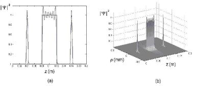
Figure 31: (a) Comparison between the intensity of the desired longitudinal function $F(z)$ and that of our Frozen Wave (FW),  $\Psi(\rho=0,z,t)$,  obtained from eq.(98). The solid line represents the function $F(z)$, and the dotted one our FW.  (b) 3D-plot of the field-intensity of the FW chosen in this case by us.

One can verify that a good agreement between the desired longitudinal behaviour and our approximate FW is already got for $N=30$. The use of higher values for $N$ can only improve the approximation.  Figure (31 b) shows the 3D-intensity of our FW, given by eq.(100). One can observe that this field possesses the desired longitudinal pattern, while being endowed with a good transverse localization.

Second example (controlling the transverse shape too):

We wish to take advantage of this example for addressing an important question:  We can expect that, for a desired longitudinal pattern of the field intensity, by choosing smaller values of the parameter $Q$ one will get FWs with narrower transverse width [for the same number of terms in the series entering eq.(100)], because of the fact that the Bessel beams in eq.(100) will possess larger transverse wave numbers, and, consequently, higher transverse concentrations.  We can verify this expectation by considering, for instance, inside the usual range $0\leq z\leq L$, the longitudinal pattern represented by the function

$$F(z)\;=\;\left\{\begin{array}[]{clr}-4\,\,\displaystyle{\frac{(z-l_{1})(z-l_{2})}{(l_{2}-l_{1})^{2}}}&{\rm for}\;\;\;l_{1}\leq z\leq l_{2}\\ \\ \;\;\;\;\;\;\;\;0&\mbox{elsewhere}\end{array}\right.\;,$$ (103)

with $l_{1}=L/2-\Delta z$ and $l_{2}=L/2+\Delta z$. Such a function has a parabolic shape, with its peak centered at $L/2$ and with longitudinal width $2\Delta z/\sqrt{2}$. By adopting $\lambda_{0}=0.632\;\mu$m (that is, $\omega_{0}=2.98\times 10^{15}\;$Hz), let us use superposition (100) with two different values of $Q$:  We shall obtain two different FWs that, in spite of having the same longitudinal intensity pattern, possess different transverse localizations. Namely, let us consider $L=0.06\,$m and $\Delta z=L/100$, and the two values $Q=0.999\,\omega_{0}/c$ and $Q=0.995\,\omega_{0}/c$. In both cases the coefficients $A_{m}$ will be the same, calculated from eq.(99) using this time the value $N=45$ in superposition (100). The results are shown in Figs.(32a) and (32b). Both FWs have the same longitudinal intensity pattern, but the one with the smaller $Q$ is endowed with a narrower transverse width.

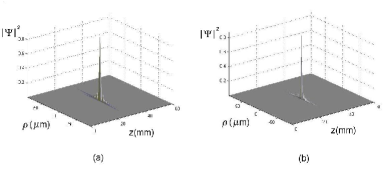
Figure 32: (a) The Frozen Wave with $Q=0.999\,\omega_{0}/c$ and $N=45$, approximately reproducing the chosen longitudinal pattern represented by eq.(103).  (b) A different Frozen wave, now with $Q=0.995\omega_{0}/c$ (but still with $N=45$) forwarding the same longitudinal pattern. We can observe that in this case (with a lower value for $Q$) a higher transverse localization is obtained.

In this way, we can get some control on the transverse spot size through the parameter $Q$.  Actually, eq.(100), which defines our FW, is a superposition of zero-order Bessel beams, and, due to this fact, the resulting field is expected to possess a transverse localization around $\rho=0$. Each Bessel beam in superposition (100) is associated with a central spot with transverse size, or width, $\Delta\rho_{m}\approx 2.4/k_{\rho\,m}$. On the basis of the expected convergence of the series (100), we can estimate the width of the transverse spot of the resulting beam as being

$$\Delta\rho\approx\frac{2.4}{k_{\rho,\,m=0}}\;=\;\frac{2.4}{\sqrt{\omega_{0}^{2}/c^{2}-Q^{2}}}\;,$$ (104)

which is the same value as that for the transverse spot of the Bessel beam with $m=0$ in superposition (100). Relation (104) can be useful: Once we have chosen the desired longitudinal intensity pattern, we can even choose the size of the transverse spot, and use relation (104) for evaluating the corresponding needed value of parameter $Q$.  For a more detailed analysis concerning the spatial resolution and residual intensity of the Frozen Waves, we refer the reader to ref.[131].

The Frozen Waves, corresponding to zero group-velocity, are a particular case of the subluminal Localized Waves.  Actually, like in the Superluminal case, the (more orthodox, in a sense) subluminal LWs can be obtained by suitable superpositions of Bessel beams. They have been till now almost neglected, however, for the mathematical difficulties met in getting analytic expressions for them, difficulties associated with the fact that the superposition integral runs now over a finite interval.  In Ref.[141] we have shown, by contrast, that one can indeed arrive at exact (analytic) solutions also in the case of general subluminal LWs, and both in the case of integration over the Bessel beams’ angular frequency $\omega$, and in the case of integration over their longitudinal wavenumber $k_{z}$.  We shall come back to this point in the following.

10.1.1 Increasing the control on the transverse shape by using higher-order Bessel beams

Here, we are going to argue that it is possible to increase even more our control on the transverse shape by using higher-order Bessel beams in our fundamental superposition (100).  This new approach can be understood and accepted on the basis of simple and intuitive arguments, which are not presented here, but can be found in ref.[131]. A brief description of that approach follows below.

The basic idea is obtaining the desired longitudinal intensity pattern not along the axis $\rho=0$, but on a cylindrical surface corresponding to $\rho=\rho^{\prime}>0$.  To do that, we first proceed as before: Once we have chosen the desired longitudinal intensity pattern $F(z)$, within the interval $0\leq z\leq L$, we calculate the coefficients $A_{m}$ as before, i.e.,  $A_{m}=(1/L)\int_{0}^{L}\,F(z)\,{\rm exp}(-i2\pi mz/L)\,{\rm d}z$,  and  $k_{\rho\,m}=\sqrt{\omega_{0}^{2}-\left(Q+2\pi m/L\right)^{2}}$.  Afterwards, we just replace the zero-order Bessel beams $J_{0}(k_{\rho\,m}\rho)$, in superposition (100), with higher-order Bessel beams, $J_{\mu}(k_{\rho\,m}\rho)$, to get

$${\Psi(\rho,z,t)\;=\;e^{-i\,\omega_{0}\,t}\,e^{i\,Q\,z}\,\sum_{m=-N}^{N}A_{m}\,J_{\mu}(k_{\rho\,m}\,\rho)\,e^{i\,\frac{2\pi}{L}m\,z}}\;,$$ (105)

From this result, and on the basis of intuitive arguments[131], we can expect that the desired longitudinal intensity pattern, initially constructed for $\rho=0$, will approximately shift to $\rho=\rho^{\prime}$, where $\rho^{\prime}$ represents the position of the first maximum of the Bessel function, i.e., the first positive root of the equation  ${\rm d}\,J_{\mu}(k_{\rho,\,m=0}\,\rho)/{\rm d}\rho)|_{\rho^{\prime}}=0$.

By such a procedure, one can obtain very interesting stationary configurations of field intensity, as “donuts”, cylindrical surfaces, and much more.

In the following example, we show how to obtain, e.g., a cylindrical surface of stationary light.  To get it, within the interval $0\leq z\leq L$, let us first select the longitudinal intensity pattern given by eq.(103), with $l_{1}=L/2-\Delta z$  and  $l_{2}=L/2+\Delta z$, and with $\Delta z=L/300$. Moreover, let us choose $L=0.05\,$m, $Q=0.998\,\omega_{0}/c$, and use $N=150$.

Then, after calculating the coefficients $A_{m}$ by eq.(99), we use to superposition (105), choosing, in this case, $\mu=4$.  According to the previous discussion, one can expect the desired longitudinal intensity pattern to appear shifted to $\rho^{\prime}\approx 5.318/k_{\rho,\,m=0}=8.47\,\mu$m, where 5.318 is the value of $k_{\rho,\,m=0}\,\rho$ for which the Bessel function $J_{4}(k_{\rho,\,m=0}\,\rho)$ assumes its maximum value, with $k_{\rho,\,m=0}=\sqrt{\omega_{0}^{2}-Q^{2}}$.  The figure 33 below shows the resulting intensity field.

In Fig.(33 a) the transverse section of the resulting beam for $z=L/2$ is shown. The transverse peak intensity is located at $\rho=7.75\,\mu$m, with a $8.5\%$ difference w.r.t. the predicted value of $8.47\,\mu$m. Figure (33 b) shows the orthogonal projection of the resulting field, which corresponds to nothing but a cylindrical surface of stationary light (or other fields).

Figure 33: (a) Transverse section at $z=L/2$ of the considered higher-order FW.  (b) Orthogonal projection of the three-dimensional intensity pattern of the same higher-order FW.

We can see that the desired longitudinal intensity pattern has been approximately obtained, shifted, as desired, from $\rho=0$ to $\rho=7.75\,\mu$m; and the resulting field resembles a cylindrical surface of stationary light with radius $7.75\,\mu$m and length $238\,\mu$m. Donut-like configurations of light (or sound) are also possible.

10.2 Stationary wavefields with arbitrary longitudinal shape in absorbing media: An extension of the method.

When propagating in a non-absorbing medium, the so-called nondiffracting waves maintain their spatial shape for long distances. However, the situation is not the same when dealing with absorbing media. In such cases, both the ordinary and the nondiffracting beams (and pulses) will suffer the same effect: an exponential attenuation along the propagation axis.  We shall present an extension[124] of the method given above, with the aim of showing that, through suitable superpositions of equal-frequency Bessel beams, it is possible to obtain even in absorbing media nondiffracting beams , whose longitudinal intensity pattern can assume any desired shape within a chosen interval $0\leq z\leq L$ of the propagation axis $z$.

As a particular example, we are going to obtain new nondiffracting beams capable to resist the loss effects, maintaining amplitude and spot size of their central core for long distances.

It is important to stress that the energy absorption by the medium continues to occur normally, but the new beams have an initial transverse field distribution, such to reconstruct (notwithstanding the presence of absorption) their central cores for distances considerably longer than the penetration depths of ordinary (nondiffracting or diffracting) beams. In this sense, the new method can be regarded as extending, for absorbing media, the self-reconstruction properties[142] that usual Localized Waves are known to possess in loss-less media.

In the same way as for lossless media, we construct a Bessel beam with angular frequency $\omega$ and axicon angle $\theta$ in the absorbing materials by superposing plane waves, with the same angular frequency $\omega$, and whose wave vectors lie on the surface of a cone with vertex angle $\theta$. The refractive index of the medium can be written as $n(\omega)=n_{{\rm R}}(\omega)+in_{{\rm I}}(\omega)$, quantity $n_{{\rm R}}$ being the real part of the complex refraction index and $n_{{\rm I}}$ the imaginary one, responsible for the absorbtion effects. For a plane wave, the penetration depth $\delta$ for the frequency $\omega$ is given by $\delta=1/\alpha=c/2\omega n_{{\rm I}}$, where $\alpha$ is the absorption coefficient.  Therefore, a zero-order Bessel beam in dissipative media can be written as  $\psi=J_{0}(k_{\rho}\rho){\rm exp}(i\beta z){\rm exp}(-i\omega t)$  with  $\beta=n(\omega)\omega\cos\theta/c=n_{{\rm R}}\omega\cos\theta/c+in_{{\rm I}}\omega\cos\theta/c\equiv\beta_{{\rm R}}+i\beta_{{\rm I}}$; $k_{\rho}=n_{{\rm R}}\omega\sin\theta/c+in_{{\rm I}}\omega\sin\theta/c\equiv k_{\rho{\rm R}}+ik_{\rho{\rm I}}$,  and so  $k_{\rho}^{2}=n^{2}\omega^{2}/c^{2}-\beta^{2}$.  Thus, it results   $\psi=J_{0}((k_{\rho{\rm R}}+ik_{\rho{\rm I}})\rho){\rm exp}(i\beta_{{\rm R}}z){\rm exp}(-i\omega t){\rm exp}(-\beta_{{\rm I}}z)$,   where $\beta_{{\rm R}}$, $k_{\rho{\rm R}}$ are the real parts of the longitudinal and transverse wave numbers, and $\beta_{{\rm I}}$, $k_{\rho{\rm I}}$ are the imaginary ones, while the absorption coefficient of a Bessel beam with axicon angle $\theta$ is given by $\alpha_{\theta}=2\beta_{{\rm I}}=2n_{{\rm I}}\omega\cos\theta/c$, its penetration depth being $\delta_{\theta}=1/\alpha_{\theta}=c/2\omega n_{{\rm I}}\cos\theta$.

Due to the fact that $k_{\rho}$ is complex, the amplitude of the Bessel function $J_{0}(k_{\rho}\rho)$ starts decreasing from $\rho=0$ till the transverse distance $\rho=1/2k_{\rho{\rm I}}$, and afterwards it starts growing exponentially. This behaviour is not physically acceptable, but one must remember that it occurs only because of the fact that an ideal Bessel beam needs an infinite aperture to be generated. However, in any real situation, when a Bessel beam is generated by finite apertures, that exponential growth in the transverse direction, starting after $\rho=1/2k_{\rho{\rm I}}$, will not occur indefinitely, stopping at a given value of $\rho$. Let us moreover emphasize that, when generated by a finite aperture of radius $R$, the truncated Bessel beam[131] possesses a depth of field $Z=R/\tan\theta$, and can be approximately described by the solution given in the previous paragraph, for $\rho<R$ and $z<Z$.

Experimentally, to guarantee that the mentioned exponential growth in the transverse direction does not even start, so as to meet only a decreasing transverse intensity, the radius $R$ of the aperture used for generating the Bessel beam should be $R\leq 1/2k_{\rho{\rm I}}$. However, as noted by Durnin et al., the same aperture has to satisfy also the relation $R\geq 2\pi/k_{\rho{\rm R}}$. From these two conditions, one can infer that, in an absorbing medium, a Bessel beam with just a decreasing transverse intensity can be generated only when the absorption coefficient is $\alpha<2/\lambda$, i.e., if the penetration depth is $\delta>\lambda/2$. The present method does refer to these cases, i.e., it is always possible to choose a suitable finite aperture size in such a way that the truncated versions of all solutions, including the general one given by eq.(111), will not develop any unphysical behaviour. Let us now outline the method[141].

Let us consider an absorbing medium with the complex refraction index $n(\omega)=n_{{\rm R}}(\omega)+in_{{\rm I}}(\omega)$, and the following superposition of $2N+1$ Bessel beams with the same frequency $\omega$:

$$\begin{array}[]{clr}\Psi(\rho,z,t)=\displaystyle{\sum_{m=-N}^{N}}A_{m}\,J_{0}\left((k_{\rho{\rm R}_{m}}+ik_{\rho{\rm I}_{m}})\rho\right)\,e^{i\,\beta_{{\rm R}_{m}}z}\,e^{-i\,\omega\,t}\,e^{-\beta_{{\rm I}_{m}}z}\;,\end{array}$$ (106)

where the $m$ are integer numbers, the $A_{m}$ are constant coefficients (yet unknown), quantities $\beta_{{\rm R}_{m}}$ and $k_{\rho{\rm R}_{m}}$ ($\beta_{{\rm I}_{m}}$ and $k_{\rho{\rm I}_{m}}$) are the real (the imaginary) parts of the complex longitudinal and transverse wave numbers of the $m$-th Bessel beam in superposition (106); the following relations being satisfied

$$k_{\rho_{m}}^{2}\;=\;n^{2}\frac{\omega^{2}}{c^{2}}-\beta_{m}^{2}$$ (107)

$$\frac{\beta_{{\rm R}_{m}}}{\beta_{{\rm I}_{m}}}\;=\;\frac{n_{{\rm R}}}{n_{{\rm I}}}$$ (108)

where $\beta_{m}=\beta_{{\rm R}_{m}}+i\beta_{{\rm I}_{m}}$, $k_{\rho_{m}}=k_{\rho{\rm R}_{m}}+ik_{\rho{\rm I}_{m}}$,  with  $k_{\rho{\rm R}_{m}}/k_{\rho{\rm I}_{m}}=n_{{\rm R}}/n_{{\rm I}}$.

Our goal is finding out the values of the longitudinal wave numbers $\beta_{m}$ and the coefficients $A_{m}$ in order to reproduce approximately, inside the interval $0\leq z\leq L$ (on the axis $\rho=0$), a freely chosen longitudinal intensity pattern that we call $|F(z)|^{2}$.  The problem for the particular case of lossless media[128,129], i.e., when $n_{{\rm I}}=0\rightarrow\beta_{{\rm I}_{m}}=0$, was solved in the previous subsection. For those cases, it was shown that the choice $\beta=Q+2\pi m/L$,  with $A_{m}=\int_{0}^{L}F(z){\rm exp}(-i2\pi mz/L)/L\,\,{\rm d}z$ can be used to provide approximately the desired longitudinal intensity pattern $|F(z)|^{2}$ in the interval $0\leq z\leq L$, and, at the same time, to regulate the spot size of the resulting beam by means of the parameter $Q$.  Such parameter, incidentally, can be also used to obtain large field-depths and moreover to inforce the linear polarization approximation to the electric field for the TE electromagnetic wave (see details in refs.[128,129]).

However, when dealing with absorbing media, the procedure described in the last paragraph does not work, due to the presence of the functions $\exp(-\beta_{{\rm I}_{m}}z)$ in the superposition (106), because in this case that series does not became a Fourier series when $\rho=0$.  On attempting to overcome this limitation, let us write the real part of the longitudinal wave number, in superposition (106), as

$$\beta_{{\rm R}_{m}}\;=\;Q+\frac{2\pi m}{L}$$ (109)

with

$$0\leq Q+\frac{2\pi m}{L}\leq n_{{\rm R}}\frac{\omega}{c}\;.$$ (110)

where inequality (110) guarantees forward propagation only, with no evanescent waves.  In this way, the superposition (106) can be written

$$\begin{array}[]{clr}\Psi(\rho,z,t)=e^{-i\,\omega\,t}\,e^{i\,Qz}\,\displaystyle{\sum_{m=-N}^{N}}A_{m}\,J_{0}\left((k_{\rho{\rm R}_{m}}+ik_{\rho{\rm I}_{m}})\rho\right)\,e^{i\,\frac{2\pi m}{L}z}\,e^{-\beta_{{\rm I}_{m}}z}\;,\end{array}$$ (111)

where, by using eq.(108), we have  $\beta_{{\rm I}_{m}}=(Q+2\pi m/L)n_{{\rm I}}/n_{{\rm R}}$,  and  $k_{\rho_{m}}=k_{\rho{\rm R}_{m}}+ik_{\rho{\rm I}_{m}}$ is given by eq.(107). Obviously, the discrete superposition (111) could be written as a continuous one (i.e., as an integral over $\beta_{{\rm R}_{m}}$) by taking $L\rightarrow\infty$, but we prefer the discrete sum due to the difficulty of obtaining closed-form solutions to the integral form.

Now, let us examine the imaginary part of the longitudinal wave numbers. The minimum and maximum values among the $\beta_{{\rm I}_{m}}$ are $(\beta_{{\rm I}})_{\rm min}=(Q-2\pi N/L)n_{{\rm I}}/n_{{\rm R}}$ and $(\beta_{{\rm I}})_{\rm max}=(Q+2\pi N/L)n_{{\rm I}}/n_{{\rm R}}$, the central one being given by $\overline{\beta}_{{\rm I}}\equiv(\beta_{{\rm I}})_{m=0}=Qn_{{\rm I}}/n_{{\rm R}}$. With this in mind, let us evaluate the ratio $\Delta=[(\beta_{{\rm I}})_{\rm max}-(\beta_{{\rm I}})_{\rm min}]/{\overline{\beta}_{{\rm I}}}=4\pi N/LQ$.  Thus, when $\Delta<<1$, there are no considerable differences among the various $\beta_{{\rm I}_{m}}$, because $\beta_{{\rm I}_{m}}\approx\overline{\beta}_{{\rm I}}$ holds for all $m$. In the same way, there are no considerable differences among the exponential attenuation factors, since $\exp(-\beta_{{\rm I}_{m}}z)\approx\exp(-\overline{\beta}_{{\rm I}}z)$. So, when $\rho=0$ the series in the r.h.s. of eq.(111) can be approximately considered a truncated Fourier series multiplied by the function $\exp(-\overline{\beta}_{{\rm I}}z)$, and, therefore, superposition (111) can be used to reproduce approximately the desired longitudinal intensity pattern $|F(z)|^{2}$ (on $\rho=0$), within $0\leq z\leq L$, when the coefficients $A_{m}$ are given by

$$A_{m}\;=\;\frac{1}{L}\,\int_{0}^{L}F(z)\,e^{\overline{\beta}_{{\rm I}}z}e^{-i\,\frac{2\pi m}{L}z}\,{\rm d}z\;,$$ (112)

the presence of the factor $\exp(\overline{\beta}_{{\rm I}}z)$ in the integrand being necessary to compensate for the factors $\exp(-\beta_{{\rm I}_{m}}z)$ in superposition (111).  Since we are adding together zero-order Bessel functions, we can expect a good field concentration around $\rho=0$.

In short, we have shown in this Section how one can get, in an absorbing medium, a stationary wave-field with a good transverse concentration, and whose longitudinal intensity pattern (on $\rho=0$) can approximately assume any desired shape $|F(z)|^{2}$ within the predetermined interval $0\leq z\leq L$. The method followed above —let us resume— is a generalization of a previous one[128,129], and consists in the superposition in eq.(111) of Bessel beams whose longitudinal wave numbers are individuated by the real and imaginary parts given in eqs.(109) and (108), respectively, while their complex transverse wave numbers are given by eq.(107). Finally, the coefficients of the superposition are given by eq.(112). The method is justified when $4\pi N/LQ<<1$: happily enough, this condition is satisfied in a great number of situations.

Regarding the generation of these new beams, once we have an apparatus capable of generating a single Bessel beam, we can just use an array of such apparatuses to generate a sum of Bessel beams, with the appropriate longitudinal wave numbers and amplitudes/phases [as specified by our method], thus producing the desired final beam. For instance, we can use[128,129] a laser illuminating an array of concentric annular apertures (located at the focus of a convergent lens), with the appropriate radii and transfer functions in order to be able to yield both the required longitudinal wave numbers (once a value for $Q$ has been chosen) and the coefficients $A_{n}$ of the fundamental superposition (111).

10.2.1 Some Examples

For generality’s sake, let us consider a hypothetical medium in which a typical XeCl excimer laser ($\lambda=308{\rm nm}\rightarrow\omega=6.12\times 10^{15}$Hz) has a penetration depth of 5 cm; i.e. an absorption coefficient $\alpha=20{\rm m}^{-1}$, and therefore $n_{{\rm I}}=0.49\times 10^{-6}$. Besides this, let us suppose that the real part of the refraction index for this wavelength is $n_{{\rm R}}=1.5$ and therefore $n=n_{{\rm R}}+in_{{\rm I}}=1.5+i\,0.49\times 10^{-6}$. Note that the value of the real part of the refractive index is not so important for us, since we are dealing with monochromatic wave fields.

A Bessel beam with $\omega=6.12\times 10^{15}$Hz and with an axicon angle $\theta=0.0141\;$rad (thus, with a transverse spot of radius $8.4\,\mu$m), when generated by an aperture, say, of radius $R=3.5\;$mm, can travel in vacuum a distance equal to $Z=R/\tan\theta=25\;$cm while resisting the diffraction effects. However, in the material medium considered here, the penetration depth of this Bessel beam would be only $z_{p}=5\;$cm. Now, let us set forth two interesting applications of the present method.

First Example: Almost Undistorted Beams in Absorbing Media.

We can use the extended method to obtain, in the same medium and for the same wavelength, an almost undistorted beam capable of preserving its spot size and the intensity of its central core for a distance many times larger than the typical penetration depth of an ordinary beam (nondiffracting or not).  To this purpose, let us suppose that, in the considered material medium, we want a beam (with $\omega=6.12\times 10^{15}$Hz) that maintains amplitude and spot size of its central core for a distance of $25\;$cm, i.e., a distance 5 times greater than the penetration depth of an ordinary beam with the same frequency. We can model this beam by choosing the desired longitudinal intensity pattern $|F(z)|^{2}$ (on $\rho=0$), within $0\leq z\leq L$, to be given by the function

$$F(z)\;=\;\left\{\begin{array}[]{clr}&1\;\;\;{\rm for}\;\;\;0\leq z\leq Z\\ &0\;\;\;\mbox{elsewhere},\end{array}\right.$$ (113)

and by putting $Z=25\;$cm, with, for example, $L=33\;$cm.

Now, one can use the Bessel beam superposition (111) to reproduce approximately the selected intensity pattern.  Let us choose $Q=0.9999\omega/c$ for the $\beta_{{\rm R}_{m}}$ in eq.(109), and $N=20$ (notice that, according to inequality (110), $N$ could assume a maximum value of $158$.)  After having chosen the values of $Q$, $L$ and $N$, the values of the complex longitudinal and transverse wave numbers of the Bessel beams happen to be defined by relations (109), (108) and (107). Eventually, we can have recourse to eq.(112), and find out the coefficients $A_{m}$ of the fundamental superposition (111), that defines the resulting stationary wave-field.  Let us just note that the condition $4\pi N/LQ<<1$ is perfectly satisfied in this case.

In Fig.(34  a) we can see the 3D field-intensity of the resulting beam. One can observe that the field possesses a good transverse localization (with a spot size smaller than $10\;\mu$m), and is capable of maintaining spot size and intensity of its central core till the desired distance (a better result could be reached by using a higher value of $N$).

Figure 34: (a) Three-dimensional field-intensity of the resulting beam. (b) The resulting beam, in an orthogonal projection and in logaritmic scale.

It is interesting to note that at that distance (25 cm), an ordinary beam would have got its initial field-intensity attenuated $148$ times.

As we said above, the energy absorption by the medium continues to occur normally; the difference is that these new beams have an initial transverse field distribution sophisticated enough to be able to reconstruct (even in the presence of absorption) their central cores, till a certain distance. For a better visualization of this field-intensity distribution and of the energy flux, we show in Fig.(34 b) the resulting beam, in an orthogonal projection and in logarithmic scale. It appears clear that the energy comes from the lateral regions, in order to reconstruct the central core of the beam. On the plane $z=0$, within the region $\rho\leq R=3.5\,$mm, there is an uncommon field intensity distribution, it being very dispersed instead of concentrated. This uncommon initial field intensity distribution is responsible for the construction of the central core of the resulting beam, and for its reconstruction all along the distance $z=25\,$cm. Due to absorption, the beam (total) energy, flowing through different $z$ planes, is not constant; but the energy flowing in the beam spot area, and the beam spot size itself, are conserved till the distance (in this case)  $z=25\,$ cm.

Second Example: Beams in absorbing media with a growing longitudinal field intensity.

Let us consider again the previous hypothetical medium, in which an ordinary Bessel beam with $\theta=0.0141\;$rad and $\omega=6.12\times 10^{15}$Hz would have a penetration depth of $5\;$cm.  We aim at constructing now a beam that, instead of possessing a constant core-intensity till the position $z=25\;$cm, presents on the contrary a (moderate) exponential growth of its intensity, till that distance ($z=25\;$cm).

Let us assume we wish to get the following longitudinal intensity pattern $|F(z)|^{2}$, in the interval $0<z<L$:

$$F(z)\;=\;\left\{\begin{array}[]{clr}&{\rm exp}(z/Z)\;\;\;{\rm for}\;\;\;0\leq z\leq Z\\ &0\;\;\;\mbox{elsewhere}\;,\end{array}\right.$$ (114)

with $Z=25\,$cm and $L=33\;$cm.  Using again $Q=0.9999\,\omega/c$, and $N=20$, we can proceed as in the first example, calculating the complex longitudinal and transverse wave numbers of the Bessel beams, and finally the coefficients $A_{m}$ of the fundamental superposition (111).

In Fig.(35) we can see the 3D field-intensity of the resulting beam. One can observe that the field presents the desired longitudinal intensity pattern, with a good transverse localization (a spot size smaller than $10\;\mu$m).

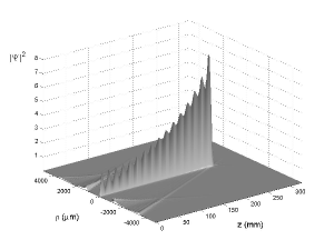
Figure 35: Three-dimensional field-intensity of the resulting beam, in AN absorbing medium, with a growing longitudinal field intensity.

Obviously, the amount of energy necessary to construct these new beams is greater than that necessary to generate an ordinary beam in a non-absorbing medium. And it is also clear that there is a limitation on the depth of field of these new beams. In the first example, for distances larger than 10 times the penetration depth of an ordinary beam, the field-intensity in the lateral regions would result to be higher than that at the core, and the field would loose the usual characteristics of a beam (transverse field concentration); not to speak of the greater energy demand.

11 Subluminal Localized Waves (or Bullets)

In this Section, abandoning for a while the subject of the so-called “Frozen Waves”, we want to face the more general problem of obtaining, in a simple way, localized (non-diffractive) subluminal pulses as exact analytic solutions to the wave equations.[141]   These new ideal subluminal solutions, which propagate without distortion in any homogeneous linear media, will be here obtained for arbitrarily chosen frequencies and bandwidths, avoiding in particular any recourse to the non-causal (backward moving) components that so frequently plague the previously known localized waves.  The new solutions are suitable superpositions of —zeroth-order, in general— Bessel beams, which can be performed either by integrating w.r.t. the angular frequency $\omega$, or by integrating w.r.t. the longitudinal wavenumber $k_{z}\,$:  Both methods are expounded in this review.  The first one will appear to be powerful enough;  we shall present the second method as well, however, since it allows dealing once more —from a different starting point— also with the limiting case of zero-speed solutions (and furnishes a new way, in terms of continuous spectra, for obtaining our Frozen Waves, so promising also from the point of view of applications).  Some attention is moreover paid to the known role of Special Relativity, and to the fact that the localized waves are expected to be transformed one into the other by suitable Lorentz Transformations.  At last, we briefly treat the case of non axially-symmetric solutions, in terms of higher order Bessel beams.  The analogous pulses with intrinsic finite energy, or merely truncated, will be considered elsewhere.  We keep fixing our attention especially on electromagnetism and optics: But let us repeat that results of the same kind are valid whenever an essential role is played by a wave-equation [like in acoustics, seismology, geophysics, elementary particle physics (as we verified even in the slightly different case of the Schroedinger equation), and also gravitation (for which we have recently got stimulating new results), and so on].

11.1 A foreword about the Subluminal Localized Waves

For self-consistency, let us repeat here the following considerations. For more than ten years, the so-called (non-diffracting) “Localized Waves” (LW), which are new solutions to the wave equations (scalar, vectorial, spinorial,…), are in fashion, both in theory and in experiment. In particular, rather well-known are the ones with luminal or Superluminal peak-velocity[143]: Like the so-called X-shaped waves (see[144, 145] and refs. therein; for a review, see, e.g., ref.[146]), which are supersonic in Acoustics[147], and Superluminal in Electromagnetism (see[148] and refs. therein).

As we know, since Bateman[149] and later on Courant & Hilbert[150], it was recognized, e.g., that luminal LWs exist, which are solutions to the wave equations. More recently, some attention[9-13] started to be paid to the (more “orthodox”, as we said) subluminal LWs too. Let us recall that all the LWs propagate without distortion —and in a self-reconstructive way[14-16]— in a homogeneous linear medium (apart from local variations): In the sense that their square magnitude keeps its shape during propagation, while local variations are shown only by its real, or imaginary, part.

As in the Superluminal case, the subluminal LWs can be obtained by suitable superpositions of Bessel beams.[141]  They have been till now almost neglected, as we know, for the mathematical difficulties met in getting analytic expressions for them, difficulties associated with the fact that the superposition integral runs over a finite interval.  We shall here re-address the question of such subluminal LWs, showing, by contrast, that one can indeed arrive at exact (analytic) solutions, both in the case of integration over the Bessel beams’ angular frequency $\omega$, and in the case of integration over their longitudinal wavenumber $k_{z}$.

As already claimed, the present work is devoted to the exact, analytic solutions: i.e., to ideal solutions.  The corresponding pulses with finite energy, or truncated, will be presented elsewhere.

Let us recall that, in the past, too much attention was not even paid to Brittingham’s 1983 paper[159], wherein he had shown the possibility of obtaining pulse-type solutions to the Maxwell equations, which propagate in free space as a new kind of speed-c “solitons”. That lack of attention was partially due to the fact that Brittingham had been able neither to get correct finite-energy expressions for such “wavelets”, nor to make suggestions about their practical production. Two years later, however, Sezginer[160] was able to obtain quasi-nondiffracting luminal pulses endowed with a finite energy.  Finite-energy pulses do no longer travel undistorted, as we do know, for an infinite distance, but can nevertheless propagate without deformation for a long field-depth, much larger than the one achieved by ordinary pulses like the gaussian ones: Cf., e.g., refs.[19-24] and refs. therein.

Only after 1985 the general theory of LWs started to be extensively developed[25-31,2,6,3], both in the case of beams and in the case of pulses. For reviews, see for instance the refs.[146, 174, 165, 163, 166] and citations therein.  For the propagation of LWs in bounded regions (like wave-guides), see refs.[33-36] and refs therein.  For the focusing of LWs, see the Second Part of this review [as well as refs.[179, 180] and quotations therein].  As to the construction of general LWs propagating in dispersive media, see refs.[39-47]; and, for lossy media, cf. ref.[158] and refs. therein.  Al last, for finite-energy, or truncated, solutions see refs.[48-50,24,3,34], and work in progress.

By now, the LWs have been experimentally produced[147, 193, 194], and are being applied in fields ranging from ultrasound scanning[195, 196, 153] to optics (for the production, e.g., of new type of tweezers[197]). All those works have demonstrated by now that nondiffracting pulses can travel with an arbitrary peak-speed $v$, that is, with $0<v<\infty$; while Brittingham and Sezginer had confined themselves to the luminal case ($v=c$) only.

As we were remarking, the Superluminal and luminal LWs have been, and are being, intensively studied; whilst the subluminal ones have been neglected: Almost all the few papers dealing with them had recourse till now to the paraxial[198] approximation[199], or to numerical simulations[154], due to the above mentioned mathematical difficulty in obtaining exact analytic expressions for subluminal pulses. Indeed, only one analytic solution was known[9-11,28,57,58], biased by the physically unconvenient facts that its frequency spectrum is very large, that it doesn’t even possess a well-defined central frequency, and, even more, that backward-travelling[168, 166] components (ordinarily called “non-causal”, since they should be entering the antenna or generator) were needed for constructing it.  Aim of the next Sections is showing, on the contrary, that subluminal localized exact solutions can be constructed with any spectra, in any frequency bands and for any bandwidths; and without employing[145, 165] any backward-travelling components.

12 A first method for constructing physically
acceptable, subluminal Localized Pulses

Axially symmetric solutions to the scalar wave equation are known to be superpositions of zero-order Bessel beams over the angular frequency $\omega$ and the longitudinal wavenumber $k_{z}$:  That is, in cylindrical co-ordinates,

$$\Psi(\rho,z,t)\;=\;\int_{0}^{\infty}\,{\rm d}\omega\,\int_{-\omega/c}^{\omega/c}\,{\rm d}k_{z}\,\overline{S}(\omega,k_{z})J_{0}\left(\rho\sqrt{\frac{\omega^{2}}{c^{2}}-k_{z}^{2}}\right)e^{ik_{z}z}e^{-i\omega t}\;,$$ (115)

where  $k_{\rho}^{2}\equiv\omega^{2}/c^{2}-k_{z}^{2}$  is the transverse wavenumber.  Quantity $k_{\rho}^{2}$ has to be positive since evanescent waves cannot come into the play.

The condition characterizing a nondiffracting wave is the existence[166, 201] of a linear relation between longitudinal wavenumber $k_{z}$ and frequency $\omega$ for all the Bessel beams entering superposition (113); that is to say, the chosen spectrum has to entail[145, 163] for each Bessel beam a linear relationship of the type:

$$\omega\;=\;v\,k_{z}+b\;\,$$ (116)

with $b\geq 0$.  Requirement (116) can be regarded also as a specific space-time coupling, implied by the chosen spectrum $\overline{S}$. Equation (116) has to be obeyed by the spectra of any one of the three possible types (subluminal, luminal or Superluminal) of nondiffracting pulses.  Let us mention that with the choice in eq.(116) the pulse re-gains its initial shape after the space-interval ${\Delta z}_{1}=2\pi v/b$.  But the more general case can be also considered[145, 189] when $b$ assumes any values $b_{m}=m\,b$ (with $m$ an integer), and the periodicity space-interval becomes ${\Delta z}_{m}={\Delta z}_{1}/m\,$.  We are referring ourselves, of course, to the real (or imaginary) part of the pulse, since its modulus is known to be endowed with rigid motion.

In the subluminal case, of interest here, the only exact solution known till recent time, represented by eq.(124) below, was the one found by Mackinnon[151]. Indeed, by taking into explicit account that the transverse wavenumber $k_{\rho}$ of each Bessel beam entering eq.(115) has to be real, it can be easily shown (as first noticed by Salo et al. for the analogous acoustic solutions[154]) that in the subluminal case $b$ cannot vanish, but must be larger than zero:  $b>0$.  Then, on using conditions (116) and $b>0$, the subluminal localized pulses can be expressed as integrals over the frequency only:

$$\Psi(\rho,z,t)\;=\;\exp{[-ib{z\over v}]}\,\int_{\omega_{-}}^{\omega_{+}}\,{\rm d}\omega\;S(\omega)\,J_{0}(\rho k_{\rho})\,\exp{[i\omega{\zeta\over v}]}\;,$$ (117)

where now

$$k_{\rho}\;=\;{1\over v}\,\sqrt{2b\omega-b^{2}-(1-v^{2}/c^{2})\omega^{2}}\;\,$$ (118)

with

$$\zeta\,\equiv\,z-vt\;\,$$ (119)

and with

$\left\{\begin{array}[]{clr}\omega_{-}\;=\;\displaystyle{{b\over{1+v/c}}}\\ \\ \omega_{+}\;=\;\displaystyle{{b\over{1-v/c}}}\end{array}\right.$ (120)

As anticipated, the Bessel beam superposition in the subluminal case results to be an integration over a finite interval of $\omega$, which does clearly shows that the backward-travelling (non-causal) components correspond to the interval $\omega_{-}<\omega<b$.  It could be noticed that eq.(117) does not represent the most general exact solution, which on the contrary is a sum[189] of such solutions for the various possible values of $b$ mentioned above: That is, for the values $b_{m}=m\,b$ with spatial periodicity ${\Delta z}_{m}={\Delta z}_{1}/m\,$.  But we can confine ourselves to solution (117) without any real loss of generality, since the actual problem is evaluating in analytic form the integral entering eq.(117). For any mathematical and physical details, see ref.[189].

Now, if one adopts the change of variable

$$\omega\,\equiv\,{b\over{1-v^{2}/c^{2}}}\;(1+{v\over c}s)\;\,$$ (121)

equation (117) becomes[154]

$$\Psi(\rho,z,t)\;=\;{b\over c}\,{v\over{1-v^{2}/c^{2}}}\,\exp{[-i{b\over v}z]}\;\exp{\left[i{b\over v}\,{1\over{1-v^{2}/c^{2}}}\,\zeta\right]}$$ (122)

$${}\times\int_{-1}^{1}\,{\rm d}s\;S(s)\,J_{0}\left({b\over c}\,{\rho\over{\sqrt{1-v^{2}/c^{2}}}}{\sqrt{1-s^{2}}}\right)\;\exp{\left[i{b\over c}{1\over{1-v^{2}/c^{2}}}\zeta s\right]}\;.$$

In the following we shall adhere —as it is an old habit of ours— to some symbols standard in Special Relativity (since the whole topic of subluminal, luminal and Superluminal LWs is strictly connected[146, 148, 202] with the principles and structure of SR [cf.[203, 204] and refs. therein], as we shall mention also in the concluding remarks which fllow below); namely:

$$\beta\equiv{v\over c}\;;\ \ \ \ \ \ \ \ \ \gamma\,\equiv\,{1\over{\sqrt{1-\beta^{2}}}}\;.$$ (123)

As already said, eq.(122) has till now yielded one analytic solution for $S(s)\,=\;$constant, only (for instance, $S(s)=1$); which means nothing but $S(\omega)\,=\;$constant: in this case one gets indeed the Mackinnon solution[151, 170, 153, 192]

$$\Psi(\rho,\zeta,\eta)\;=\;2{b\over c}v\,\gamma^{2}\,{\exp{\left[i{b\over c}\,\beta\gamma^{2}\;\eta\right]}}$$ (124)

$${}\times{\rm sinc}\ {\sqrt{{b^{2}\over c^{2}}\,\gamma^{2}\left(\rho^{2}+\gamma^{2}\;\zeta^{2}\right)}}\;,$$

which however, for its above-mentioned drawbacks, is endowed with little physical and practical interest.  In eq.(124) the ${\rm sinc}$ function has the ordinary definition

$${\rm sinc}\ x\,\equiv\,(\sin\;x)/x\;,$$

and

$$\eta\,\equiv\,z-Vt,\ \ \ \ \ \ \ {\rm with}\ \ V\equiv{c^{2}\over v}\;,$$ (125)

where $V$ and $v$ are related by the de Broglie relation.  [Notice that $\Psi$ in eq.(124), and in the following ones, is eventually a function (besides of $\rho$) of $z,t$ via $\zeta$ and $\eta$, both functions of $z$ and $t\;$].

However, we can construct by a very simple method new subluminal pulses corresponding to whatever spectrum, and devoid of backward-moving (i.e., “entering”) components, just by taking advantage of the fact that in our equation (122) the integration interval is finite: that it, by transforming it in a good, instead of a harm. Let us first observe that eq.(122) doesn’t admit only the already known analytic solution corresponding to $S(s)=\;$constant, and more in general to $S(\omega)\,=\;$constant, but it will also yield an exact, analytic solution for any exponential spectra of the type

$$S(\omega)\;=\;\exp{[{i2n\pi\omega\over\Omega}]}\;,$$ (126)

with $n$ any integer number, which means for any spectra of the type $S(s)=\exp{[in\pi/\beta]}\,\exp{[in\pi s]}$,  as can be easily seen by checking the product of the various exponentials entering the integrand.  In eq.(126) we have set

$$\Omega\,\equiv\,{\omega_{+}}-{\omega_{-}}\;.$$

The solution writes in this more general case:

$$\Psi(\rho,\zeta,\eta)\;=\;2b\beta\,\gamma^{2}\,\exp{\left[i{b\over c}\,\beta\,\gamma^{2}\,\eta\right]}$$ (127)

$${}\times\exp{[in{\pi\over\beta}]}\ {\rm sinc}\ {\sqrt{{b^{2}\over c^{2}}\,\gamma^{2}\,\rho^{2}+\left({b\over c}\,\gamma^{2}\,\zeta+n\pi\right)^{2}}}\;.$$

Let us explicitly notice that also in eq.(127) quantity $\eta$ is defined as in Eqs.(125) above, where $V$ and $v$ obey the de Broglie relation $vV=c^{2}$, the subluminal quantity $v$ being the velocity of the pulse envelope, and $V$ playing the role (in the envelope’s interior) of a Superluminal phase velocity.

The next step, as anticipated, consists just in taking advantage of the finiteness of the integration limits for expanding any arbitrary spectra $S(\omega)$ in a Fourier series in the interval $\omega_{-}\leq\omega\leq\omega_{+}\;$:

$$S(\omega)\;=\;\sum_{n=-\infty}^{\infty}\,A_{n}\,\exp{[+in{2\pi\over\Omega}\omega]}\;,$$ (128)

where (we went back, now, from the $s$ to the $\omega$ variable):

$$A_{n}\;=\;{1\over\Omega}\,\int_{\omega_{-}}^{\omega_{+}}{\rm d}\omega\,S(\omega)\,\exp{[-in{2\pi\over\Omega}\omega]}\;\,$$ (129)

quantity $\Omega$ being defined as above.

Then, on remembering the special solution (127), we can infer from expansion (126) that, for any arbitrary spectral function $S(\omega)$, one can work out a rather general axially-symmetric analytic solution for the subluminal case:

$$\Psi(\rho,\zeta,\eta)\;=\;2b\beta\,\gamma^{2}\,{\exp{\left[i{b\over c}\,\beta\,\gamma^{2}\;\eta\right]}}$$ (130)

$${}\times\sum_{n=-\infty}^{\infty}\,A_{n}\,\exp{[in{\pi\over\beta}]}\ {\rm sinc}\ {\sqrt{{b^{2}\over c^{2}}\,\gamma^{2}\rho^{2}+\left({b\over c}\gamma^{2}\;\zeta+n\pi\right)^{2}}}\;,$$

in which the coefficients $A_{n}$ are still given by eq.(129). Let us repeat that our solution is expressed in terms of the particular equation (127), which is a “Mackinnon-type” solution.

The present approach presents many advantages. We can easily choose spectra localized within the prefixed frequency interval (optical waves, microwaves, etc.) and endowed with the desired bandwidth. Moreover, as we have seen, spectra can now be chosen such that they have zero value in the region $\omega_{-}\leq\omega\leq b$, which is responsible for the backward-travelling components of the subluminal pulse.

Let us stress that, even when the adopted spectrum $S(\omega)$ does not possess a known Fourier series (so that the coefficients $A_{n}$ cannot be exactly evaluated via eq.(129)), one can calculate approximately such coefficients without meeting any problem, since our general solutions (130) will still be exact solutions.

Let us set forth some examples.

12.1 Some Examples

In general, optical pulses generated in the lab possess a spectrum centered at some frequency value, $\omega_{0}$, called the carrier frequency.  The pulses can be, for instance, ultra-short, when $\Delta\omega/\omega_{0}\geq 1$; or quasi-monochromatic, when $\Delta\omega/\omega_{0}<<1$, where $\Delta\omega$ is the spectrum bandwidth.

These kinds of spectra can be mathematically represented by a gaussian function, or functions with similar behaviour.

First Two Examples:

Let us first consider a gaussian spectrum

$$S(\omega)\;=\;\frac{a}{\sqrt{\pi}}\exp{[-a^{2}(\omega-\omega_{0})^{2}]}$$ (131)

whose values are negligible outside the frequency interval $\omega_{-}<\omega<\omega_{+}$ over which the Bessel beams superposition in eq.(117) is made, it being $\omega_{-}=b/(1+\beta)$ and $\omega_{+}=b/(1-\beta)$.  Of course, relation (116) has still to be satisfied, with $b>0$, for getting an ideal subluminal localized solution.  Notice that, with spectrum (131), the bandwidth (actually, the FWHM) results to be $\Delta\omega=2/a$.  Let us emphasize that, once $v$ and $b$ have been fixed, the values of $a$ and $\omega_{0}$ can afterwards be selected in order to kill the backward-travelling components, that correspond, as we know, to $\omega<b\;$.

The Fourier expansion in eq.(128), which yields, with the above spectral function (131), the coefficients

$$A_{n}\,\simeq\,\displaystyle{{{1}\over{W}}}\,\exp{[-in{2\pi\over\Omega}\omega_{0}]}\;\exp{[{{-n^{2}\pi^{2}}\over{a^{2}W^{2}}}]}\;,$$ (132)

constitutes an excellent representation of the gaussian spectrum (131) in the interval $\omega_{-}<\omega<\omega_{+}$ (provided that, as we requested, our gaussian spectrum does get negligible values outside the frequency interval $\omega_{-}<\omega<\omega_{+}$).

In other words, on choosing a pulse velocity $v<c$ and a value for the parameter $b$, a subluminal pulse with the above frequency spectrum (131) can be written as eq.(129), with the coefficients $A_{n}$ given by eq.(132): the evaluation of such coefficients $A_{n}$ being rather simple.  Let us repeat that, even if the values of the $A_{n}$ are obtained via a (rather good, by the way) approximation, we based ourselves on the exact solution eq.(130).

One can, for instance, obtain exact solutions representing subluminal pulses for optical frequencies. Let us get the subluminal pulse with velocity $v=0.99\;c$, carrier angular frequency $\omega_{0}=2.4\times 10^{15}\;$Hz (that is, $\lambda_{0}=0.785\;\mu$m) and bandwidth (FWHM) $\Delta\omega=\omega_{0}/20=1.2\times 10^{14}\;$Hz, which is an optical pulse of $24$ fs (which is the FWHM of the pulse intensity).  For a complete pulse characterization, one has to choose the value of the frequency $b$:  let it be $b=3\times 10^{13}\;$Hz;  as a consequence one has $\omega_{-}=1.507\times 10^{13}\;$Hz and $\omega_{+}=3\times 10^{15}\;$Hz.  [This is exactly a case in which the considered pulse is not plagued by the presence of backward-travelling components, since the chosen spectrum possesses totally negligible values for $\omega<b$].  The construction of the pulse does already result satisfactory when considering about 51 terms ($-25\leq n\leq 25$) in the series entering eq.(130).

Figures 36 show our pulse, evaluated by summing the mentioned fifty-one terms. Namely: Fig.(36a) depicts the orthogonal projection of the pulse intensity;  Fig.(36b) shows the three-dimensional intensity pattern of the real part of the pulse, which reveals the carrier wave oscillations.

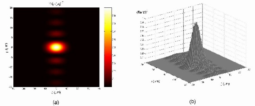
Figure 36: (a) The intensity orthogonal projection for the pulse corresponding to eqs.(131,132) in the case of an optical frequency (see the text);  (b) The three-dimensional intensity pattern of the real part of the same pulse, which reveals the carrier wave oscillations.

Let us stress that the ball-like shape for the field intensity should be typically associated with all the subluminal LWs, while the typical Superluminal ones are known to be X-shaped[144, 148, 202], as predicted since long by special relativity in its “non-restricted” version: See refs.[203, 204, 148, 146] and refs therein.

A second spectrum $S(\omega)$ would be, for instance, the “inverted parabola” one, centered at the frequency $\omega_{0}$:  that is,

$$S(\omega)\;=\;\left\{\begin{array}[]{clr}{\frac{-4\,[\omega-(\omega_{0}-\Delta\omega/2)][\omega-(\omega_{0}+\Delta\omega/2)]}{\Delta\omega^{2}}}&{\rm for}\;\;\;\omega_{0}-\Delta\omega/2\leq\omega\leq\omega_{0}+\Delta\omega/2\\ \\ \;\;\;\;\;\;0&{\rm otherwise}\ ,\end{array}\right.$$ (133)

where $\Delta\omega$, the distance between the two zeros of the parabola, can be regarded as the spectrum bandwidth.  One can expand $S(\omega)$, given in eq.(133), in the Fourier series (128), for $\omega_{-}\leq\omega\leq\omega_{+}\;$, with coefficients $A_{n}$ that —even if straightforwardly calculable— results to be complicated, so that we skip reporting them here explicitly.  Let us here only mention that spectrum (133) may be easily used to get, for instance, an ultrashort (femtasecond) optical non-diffracting pulse, with satisfactory results even when considering very few terms in expansion (128).

Third Example:

As a third interesting example, let us consider the very simple case when —within the integration limits $\omega_{-}$, $\omega_{+}$— the complex exponential spectrum (124) is replaced by the real function (still linear in $\omega$)

$$S(\omega)\;=\;\frac{a}{1-\exp{[-a(\omega_{+}-\omega_{-})]}}\,\exp{[a(\omega-\omega_{+}]}\;,$$ (134)

with $a$ a positive number [for $a=0$ one goes back to the Mackinnon case]. Spectrum (134) is exponentially concentrated in the proximity of $\omega_{+}$, where it reaches its maximum value; and becomes more and more concentrated (on the left of $\omega_{+}$, of course) as the arbitrarily chosen value of $a$ increases, its frequency bandwidth being $\Delta\omega=1/a$. Let us recall that, on their turn, quantities $\omega_{+}$ and $\omega_{-}$ depend on the pulse velocity $v$ and on the arbitrary parameter $b$.

By performing the integration as in the case of spectrum (126), instead of solution (127) in the present case one eventually gets the solution

$$\Psi(\rho,\zeta,\eta)\;=\;\frac{2ab\beta\gamma^{2}\,\exp{[ab\gamma^{2}]}\,\exp{[-a\omega_{+}]}}{1-\exp{[-a(\omega_{+}-\omega_{-})]}}$$ (135)

$${}\times\exp{\left[i{b\over c}\,\beta\,\gamma^{2}\,\eta\right]}\ {\rm sinc}{\left[{b\over c}\,\gamma^{2}\;{\sqrt{\gamma^{-2}\,\rho^{2}-(av+i\zeta)^{2}}}\right]}\;.$$

After Mckinnon’s, this eq.(135) appears to be the simplest closed-form solution, since both of them do not need any recourse to series expansions. In a sense, our solution (135) may be regarded as the subluminal analogue of the (Superluminal) X-wave solution; a difference being that the standard X-shaped solution has a spectrum starting with 0, where it assumes its maximum value, while in the present case the spectrum starts at $\omega_{-}$ and gets increasing afterwards, till $\omega_{+}$.  More important is to observe that the gaussian spectrum has a priori two advantages w.r.t. eq.(134): It may be more easily centered around any value $\omega_{0}$ of $\omega$, and, when increasing its concentration in the surroundings of $\omega_{0}$, the spot transverse width does not increase indefinitely, but tends to the spot-width of a Bessel beam with $\omega=\omega_{0}$ and $k_{z}=(\omega_{0}-b)/V$, at variance with what happens for spectrum (134).  Anyway, solution (135) is noticeable, since it is really the simplest one.

Figure 37 shows the intensity of the real part of the subluminal pulse corresponding to this spectrum, with $v=0.99\;c$, with $b=3\times 10^{13}\;$Hz (which result in $\omega_{-}=1.5\times 10^{13}\;$Hz and $\omega_{+}=3\times 10^{15}\;$Hz), and with $\Delta\omega/\omega_{+}=1/100$ (i.e., $a=100$). This is an optical pulse of $0.2$ ps.

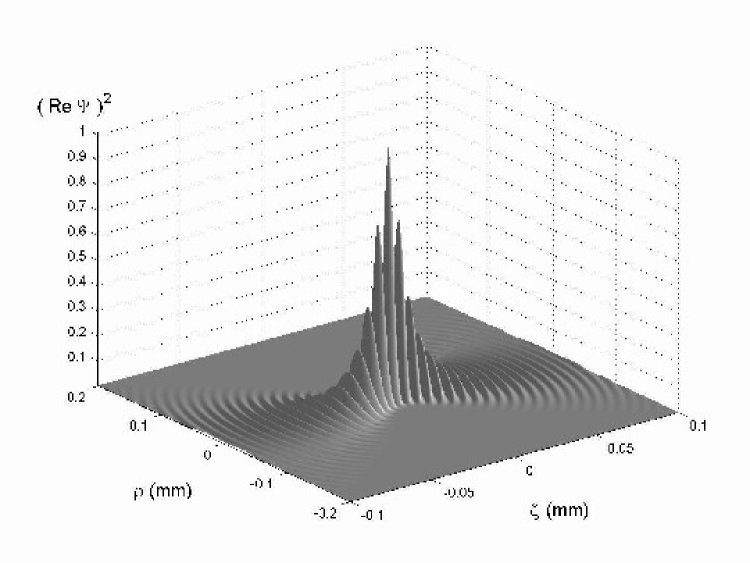
Figure 37: The intensity of the real part of the subluminal pulse corresponding to spectrum (134), with $v=0.99\;c$, with $b=3\times 10^{13}\,$Hz (which result in $\omega_{-}=1.5\times 10^{13}\;$Hz and $\omega_{-}=3\times 10^{15}\;$Hz), and with $\Delta\omega/\omega_{+}=1/100$ (i.e., $a=100$).

13 A second method for constructing
subluminal Localized Pulses

The previous method appears to be very efficient for finding out analytic subluminal LWs, but it looses its validity in the limiting case $v\rightarrow 0$, since for $v=0$ it is $\omega_{-}\equiv\omega_{+}$ and the integral in eq.(117) degenerates, furnishing a null value.  By contrast, we are interested also in the $v=0$ case, since it corresponds, as we already know, to some of the most interesting, and potentially useful, LWs:  Namely, to the stationary solutions to the wave equations endowed with a static envelope, and that we have called “Frozen Waves”.

Before going on, let us recall that the theory of Frozen Waves was initially developed in refs.[191, 205], by having recourse to discrete superpositions in order to bypass the need of numerical simulations.  In the case of continuous superpositions, some numerical simulations were performed in refs.[206].  However, the method presented in this Section does allow finding out analytic exact solutions (without any further need of numerical simulations) even for Frozen Waves consisting in continuous superpositions. Actually, we are going to see that the present method works whatever is the chosen field-intensity shape, also in regions with size of the order of the wavelength.

It is possible to get such results by starting again from eq.(115), with constraint (114), but going on —this time— to integrals over $k_{z}$, instead of over $\omega$.  It is enough to write relation (116) in the form

$k_{z}\;=\;\displaystyle{{1\over v}\,(\omega-b)}$ (116’)

for expressing the exact solutions (115) as

$$\Psi(\rho,z,t)\;=\;\exp{[-ibt]}\;\int_{k_{z}{\rm min}}^{k_{z}{\rm max}}\,{\rm d}k_{z}\;S(k_{z})\,J_{0}(\rho k_{\rho})\,\exp{[i\zeta k_{z}]}\;,$$ (136)

with

$\left\{\begin{array}[]{clr}k_{z}{\rm min}\;=\;\displaystyle{{-b\over c}\,{1\over{1+\beta}}}\\ \\ k_{z}{\rm max}\;=\;\displaystyle{{b\over c}\,{1\over{1-\beta}}}\end{array}\right.$ (135)

and with

$${k_{\rho}}^{2}\;=\;-{k_{z}^{2}\over\gamma^{2}}+2{b\over c}\beta k_{z}+{b^{2}\over c^{2}}\;,$$ (138)

where quantity $\zeta$ is still defined according to eq.(119), always with $v<c$.

One can show that the unique exact solution previously known[151] may be rewritten in form (136) with $S(k_{z})=\;$constant.  Then, on following the same procedure exploited in our first method (previous Section), one can find out new exact solutions corresponding to

$$S(k_{z})\;=\;\exp{[{i2n\pi k_{z}\over K}]}\;,$$ (139)

where

$$K\,\equiv\,k_{z}{\rm max}-{k_{z}{\rm min}}\;,$$

by performing the change of variable [analogous, in its finality, to the one in eq.(121)]

$$k_{z}\,\equiv\,{b\over c}\,\gamma^{2}\,(s+\beta)\;.$$ (140)

At the end, the exact subluminal solution corresponding to spectrum (139) results to be

$$\Psi(\rho,\zeta,\eta)\;=\;2\,{b\over c}\,\gamma^{2}\,\exp{[i{b\over c}\,\beta\,\gamma^{2}\,\eta]}$$ (141)

$${}\times\exp{[in\pi\beta]}\ {\rm sinc}\ {\sqrt{{b^{2}\over c^{2}}\,\gamma^{2}\,\rho^{2}+\left({b\over c}\,\gamma^{2}\,\zeta+n\pi\right)^{2}}}\;,$$

We can again observe that any spectra $S(k_{z})$ can be expanded, in the interval $k_{z}{\rm min}<k_{z}<k_{z}{\rm max}$, in the Fourier series:

$$S(k_{z})\;=\;\sum_{n=-\infty}^{\infty}\,A_{n}\,\exp{[+in{2\pi\over K}k_{z}]}\;,$$ (142)

with coefficients given now by

$$A_{n}\;=\;{1\over K}\,\int_{k_{z}{\rm min}}^{k_{z}{\rm max}}{\rm d}k_{z}\,S(k_{z})\,\exp{[-in{2\pi\over K}k_{z}]}\;\,$$ (143)

quantity $K$ having been defined before.

At the end of the whole procedure, the general exact solution representing a subluminal LW, for any spectra $S(k_{z})$, can be eventually written

$$\Psi(\rho,\zeta,\eta)\;=\;2\,{b\over c}\,\gamma^{2}\,\exp{[i{b\over c}\,\beta\,\gamma^{2}\,\eta]}$$ (144)

$${}\times\sum_{n=-\infty}^{\infty}\,A_{n}\,\exp{[in\pi\beta]}\ {\rm sinc}\ {\sqrt{{b^{2}\over c^{2}}\,\gamma^{2}\,\rho^{2}+\left({b\over c}\,\gamma^{2}\,\zeta+n\pi\right)^{2}}}\;,$$

whose coefficients are expressed in eq.(143), and where quantity $\eta$ is defined as above, in eq.(125).

Interesting examples could be easily worked out, as we did at the end of the previous Section.

14 Stationary solutions with zero-speed envelopes

Here, we shall refer ourselves to the (second) method, expounded in the previous Section.  Our solution (144), for the case of envelopes at rest, that is, in the case $v=0$ [which implies $\zeta=z$], becomes

$\Psi(\rho,z,t)\;=\;\displaystyle{2\,{b\over c}\;\exp{[-ibt]}\;\sum_{n=-\infty}^{\infty}\,A_{n}\ {\rm sinc}\ {\sqrt{{b^{2}\over c^{2}}\,\rho^{2}+\left({b\over c}\,z+n\pi\right)^{2}}}}\;,$ (145)

with coefficients $A_{n}$ given by eq.(143) with $v=0$, so that its integration limits simplify into $-b/c$ and $b/c$, respectively. Thus, one gets

$A_{n}\;=\;\displaystyle{{c\over{2b}}\,\int_{-b/c}^{b/c}{\rm d}k_{z}\,S(k_{z})\,\exp{[-in{c\pi\over b}k_{z}]}}\;.$ (143’)

Equation (145) is a new exact solution, corresponding to stationary beams with a static intensity envelope.  Let us observe, however, that even in this case one has energy propagation, as it can be easily verified from the power flux $\mbox{\boldmath$S$}_{\rm s}=-\mbox{\boldmath$\nabla$}\Psi_{\cal R}\ \partial\Psi_{\cal R}/\partial t$ (scalar case) or from the Poynting vector $\mbox{\boldmath$S$}_{\rm v}=(\mbox{\boldmath$E$}\wedge\mbox{\boldmath$H$})$ (vectorial case: the condition being that $\Psi_{\cal R}$ be a single component, $A_{z}$, of the vector potential $A$).[148]  We have indicated by $\Psi_{\cal R}$ the real part of $\Psi$.  For $v=0$, eq.(116) becomes

$$\omega\;=\;b\,\equiv\,\omega_{0}\;,$$

so that the particular subluminal waves endowed with null velocity are actually monochromatic beams.

It may be stressed that the present (second) method does yield exact solutions, without any need of the paraxial approximation, which, on the contrary, is so often used when looking for expressions representing beams, like the gaussian ones.  Let us recall that, when having recourse to the paraxial approximation, the obtained beam expressions are valid only when the envelope sizes (e.g., the beam spot) vary in space much more slowly than the beam wavelength. For instance, the usual expression for a gaussian beam[198] holds only when the beam spot $\Delta\rho$ is much larger than $\lambda_{0}\equiv\omega_{0}/(2\pi c)=b/(2\pi c)$: so that those beams cannot be very much localized.  By contrast, our method overcomes such problems, since we have seen that it yields exact expressions for (well localized) beams with sizes of the order of their wavelength.  Notice, moreover, that the already-known exact solutions —for instance, the Bessel beams— are nothing but particular cases of our solution (145).

An example:  On choosing (with $0\leq q_{-}<q_{+}\leq 1$) the spectral double-step function

$S(k_{z})\;=\;\left\{\begin{array}[]{clr}\displaystyle{\frac{c}{\omega_{0}(q_{+}-q_{-})}}&{\rm for}\ q_{-}\omega_{0}/c\leq k_{z}\leq q_{+}\omega_{0}/c\\ \\ 0&{\rm elsewhere}\;,\end{array}\right.$ (146)

the coefficients of eq.(145) become

$A_{n}\;=\;\displaystyle{\frac{ic}{2\pi n\omega_{0}(q_{+}-q_{-})}\;\left[e^{-iq_{+}\pi n}-e^{-iq_{-}\pi n}\right]}\;.$ (147)

The double-step spectrum (146) corresponds, with regard to the longitudinal wave number, to the mean value $\overline{k}_{z}=\omega_{0}(q_{+}+q_{-})/2c$  and to the width $\Delta k_{z}=\omega_{0}(q_{+}-q_{-})/c$. From such relations, it follows that $\Delta k_{z}/\overline{k}_{z}=2(q_{+}-q_{-})/(q_{+}+q_{-})$.

For values of $q_{-}$ and $q_{+}$ that do not satisfy the inequality $\Delta k_{z}/\overline{k}_{z}<<1$, the resulting solution will be a non-paraxial beam.

Figures 38 show the exact solution corresponding to $\omega_{0}=1.88\times 10^{15}\;$Hz (i.e., $\lambda_{0}=1\;\mu$m), and to $q_{-}=0.3$, and to $q_{+}=0.9$:  It results to be a beam with a spot-size diameter of $0.6\;\mu$m, and, moreover, with a rather good longitudinal localization.  In the case of Eqs.(144, 145), about 21 terms ($-10\leq n\leq 10$) in the sum entering eq.(143) are quite enough for a good evaluation of the series. The beam considered in this example is highly non-paraxial (with $\Delta k_{z}/\overline{k}_{z}=1$ ), and therefore couldn’t have been obtained by ordinary gaussian beam solutions (which are valid in the paraxial regime only).

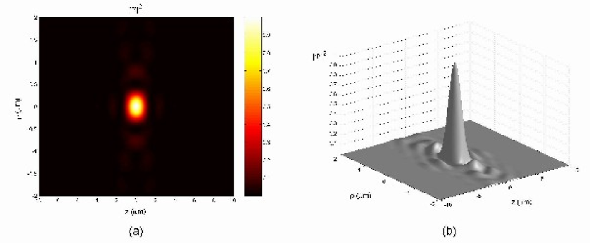
Figure 38: (a) Orthogonal projection of the three-dimensional intensity pattern of the beam (a null-speed subluminal wave) corresponding to spectrum (146);  (b) 3D plot of the field intensity. The beam considered in this example is highly non-paraxial.

14.1 A new approach to the “Frozen Waves”

Let us now emphasize that a noticeable property of the present method is that it allows a spatial modeling even of monochromatic fields (that correspond to envelopes at rest; so that, in the electromagnetic cases, one can speak, e.g., of the modeling of “light-fields at rest”).

Let us recall that such a modelling —rather interesting, especially for applications[197]— was already performed in refs.[191, 205, 158], and has been exploited at the beginning of our Third Part [cf. eqs.(99, 100)], in terms of discrete superpositions of Bessel beams. And the stationary fields with static envelopes have been called “Frozen Waves” (FW) by us.

But the method presented in the last Sections allows us to make use of continuous superpositions, in order to get a predetermined longitudinal (on-axis) intensity pattern, inside a desired space interval $0<z<L$.  In fact, the continuous superposition, analogous to eq.(100), now writes

$\Psi(\rho,z,t)\;=\;\displaystyle{e^{-i\omega_{0}t}\;\int_{-\omega_{0}/c}^{\omega_{0}/c}{\rm d}k_{z}\ S(k_{z})\ J_{0}(\rho k_{\rho})\ e^{izk_{z}}}\;,$ (148)

which is nothing but the previous eq.(136) with $v=0$ (and therefore $\zeta=z$).  In other words, eq.(148) does just represent a null-speed subluminal wave.  To be clearer, let us recall once more that the FWs were expressed in the past as discrete superposition because it was not known at that time how to treat analytically a continuous superposition like (148).  We are now able, however, to extend the previous approach to FWs to the case of integrals: without numerical simulations, but in terms once more of analytic solutions.

Indeed, the exact solution of eq.(148) is given by eq.(145), with coefficients (143’); and one can choose the spectral function $S(k_{z})$ in such a way that $\Psi$ assumes the on-axis pre-chosen static intensity pattern $|F(z)|^{2}$.  Namely, the equation to be satisfied by $S(k_{z})$, to such an aim, comes out by associating eq.(148) with the requirement $|\Psi(\rho=0,z,t)|^{2}=|F(z)|^{2}$, which entails the integral relation

$\displaystyle{\int_{-\omega_{0}/c}^{\omega_{0}/c}{\rm d}k_{z}\;S(k_{z})\;e^{izk_{z}}}\;=\;F(z)\;.$ (149)

Equation (149) would be trivially solvable in the case of an integration between $-\infty$ and $+\infty$, since it would merely be a Fourier transformation; but obviously this is not the case, because its integration limits are finite. Actually, there are functions $F(z)$ for which eq.(149) is not solvable at all, in the sense that no spectra $S(k_{z})$ exist obeying the last equation.  For instance, if we consider the Fourier expansion

$F(z)\;=\;\displaystyle{\int_{-\infty}^{\infty}}{\rm d}k_{z}\;\widetilde{S}(k_{z})\;e^{izk_{z}}\;,$

when $\widetilde{S}(k_{z})$ does assume non-negligible values outside the interval $-\omega_{0}/c<k_{z}<\omega_{0}/c$, then in eq.(149) no $S(k_{z})$ can forward that particular $F(z)$ as a result.

However, way-outs can be devised, such that one can nevertheless find out a function $S(k_{z})$ that approximately (but satisfactorily) complies with eq.(149).

The first way-out consists in writing $S(k_{z})$ in the form

$S(k_{z})\;=\;\displaystyle{{1\over K}\;\sum_{n=-\infty}^{\infty}\,F\left({{2n\pi}\over K}\right)\;e^{-i2n\pi k_{z}/K}}\;,$ (150)

where, as before, $K=2\omega_{0}/c$. Then, one can easily verify eq.(150) to guarantee that the integral in eq.(149) yields the values of the desired $F(z)$ at the discrete points  $z=2n\pi/K$.  Indeed, the Fourier expansion (150) is already of the same type as eq.(142), so that in this case the coefficients $A_{n}$ of our solution (145), appearing in eq.(143’), do simply become

$A_{n}\;=\;\displaystyle{{1\over K}\;F(-{{2n\pi}\over K})}\;.$ (151)

This is a powerful way for obtaining a desired longitudinal (on-axis) intensity pattern, especially for tiny spatial regions, because it is not necessary to solve any integral to find out the coefficients $A_{n}$, which by contrast are given directly by eq.(151).

Figures 39 depict some interesting applications of this method. A few desired longitudinal intensity patterns $|F(z)|^{2}$ have been chosen, and the corresponding Frozen Waves calculated by using eq.(145) with the coefficients $A_{n}$ given in eq.(151). The desired patterns are enforced to exist within very small spatial intervals only, in order to show the capability of the method to model[141] the field intensity shape also under such strict requirements.

In the four examples below, we considered a wavelength $\lambda=0.6\;\mu$m, which corresponds to $\omega_{0}=b=3.14\times 10^{15}\;$Hz.

The first longitudinal (on-axis) pattern considered by us is that given by

$$F(z)\;=\;\left\{\begin{array}[]{clr}\displaystyle{e^{a(z-Z)}}&{\rm for}\;\;\;0\leq z\leq Z\\ \\ \;\;\;\;\;\;\;\;0&\mbox{elsewhere}\;,\end{array}\right.$$

i.e., a pattern with an exponential increase, starting from $z=0$ untill $z=Z$. The chosen values of $a$ and $Z$ are $Z=10\;\mu$m and $a=3/Z$. The intensity of the corresponding Frozen Wave is shown in Fig.(39a).

The second longitudinal pattern (on-axis) taken into consideration is the gaussian one, given by

$$F(z)\;=\;\left\{\begin{array}[]{clr}\displaystyle{e^{-q(\frac{z}{Z})^{2}}}&{\rm for}\;\;\;-Z\leq z\leq Z\\ \\ \;\;\;\;\;\;\;\;0&\mbox{elsewhere}\;,\end{array}\right.$$

with $q=2$ and $Z=1.6\;\mu$m. The intensity of the corresponding Frozen Wave is shown in Fig.(39b).

In the third example, the desired longitudinal pattern is supposed to be a super-gaussian:

$$F(z)\;=\;\left\{\begin{array}[]{clr}\displaystyle{e^{-q(\frac{z}{Z})^{2m}}}&{\rm for}\;\;\;-Z\leq z\leq Z\\ \\ \;\;\;\;\;\;\;\;0&\mbox{elsewhere}\;,\end{array}\right.$$

where $m$ controls the edge sharpness. Here we have chosen $q=2$, $m=4$ and $Z=2\ \mu$m.  The intensity of the Frozen Wave obtained in this case is shown in Fig.(39c).

Finally, in the fourth example, let us choose the longitudinal pattern as being the zero-order Bessel function

$$F(z)\;=\;\left\{\begin{array}[]{clr}J_{0}(q\,z)&{\rm for}\;\;\;-Z\leq z\leq Z\\ \\ \;\;\;\;\;\;\;\;0&\mbox{elsewhere}\;,\end{array}\right.$$

with $q=1.6\times 10^{6}\;\rm{m}^{-1}$ and $Z=15\;\mu$m. The intensity of the corresponding Frozen Wave is shown in Fig.(39d).

Let us observe that any static envelopes of this type can be easily transformed into propagating pulses by the mere application of Lorentz transformations.

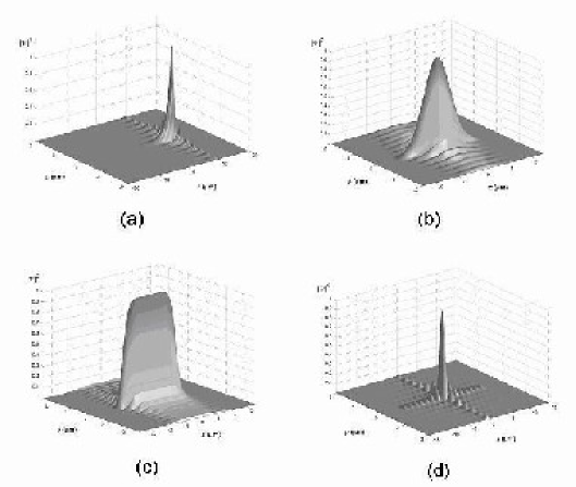
Figure 39: Frozen Waves with the on-axis longitudinal field pattern chosen as: (a) Exponential;  (b) Gaussian;  (c) Super-gaussian;  (d) Zero order  Bessel function

Another way-out exists for evaluating $S(k_{z})$, based on the assumption that

$S(k_{z})\,\simeq\,\widetilde{S}(k_{z})\;,$ (152)

which consitutes a good approximation whenever $\widetilde{S}(k_{z})$ assumes negligible values outside the interval $[-\omega_{0}/c,\ \omega_{0}/c]$.  In such a case, one can have recourse to the method associated with eq.(142) and expand $\widetilde{S}(k_{z})$ itself in a Fourier series, getting eventually the relevant coefficients $A_{n}$ by eq.(143).  Let us recall that it is still $K\equiv k_{z}{\rm max}-k_{z}{\rm min}=2\omega_{0}/c$.

It is worthwhile to call attention to the circumstance that, when constructing FWs in terms of a sum of discrete superpositions of Bessel beams (as it has been done by us in the Second part of this work, and in refs.[191, 205, 158, 197]), it was easy to obtain extended envelopes like, e.g., “cigars”: Where “easy” means by using only a few few terms of the sum. By contrast, when we construct FWs —following this Section— as continuous superpositions, then it is easy to get highly localized (concentrated) envelopes.  Let us explicitly mention, moreover, that the method presented in this Section furnishes FWs that are no longer periodic along the $z$-axis (a situation that, with our old method[191, 205, 158], was obtainable only when the periodicity interval tended to infinity).

15 The role of Special Relativity, and of Lorentz Transformations

Strict connections exist between, on one hand, the principles and structure of Special Relativity and, on the other hand, the whole subject of subluminal, luminal, Superluminal Localized Waves, in the sense that it is expected since long time that a priori they are transformable one into the other via suitable Lorentz transformations (cf. refs.[203, 204, 207], besides work of ours in progress).^♡

Let us first confine ourselves to the cases faced in this Third Part. Our subluminal localized pulses, that may be called “wave bullets”, behave as particles: Indeed, our subluminal pulses [as well as the luminal and Superluminal (X-shaped) ones, that have been amply investigated in the past literature] do exist as solutions of any wave equations, ranging from electromagnetism and acoustics or geophysics, to elementary particle physics (and even, as we discovered recently, to gravitation physics).  From the kinematical point of view, the velocity composition relativistic law holds also for them.  The same is true, more in general, for any localized waves (pulses or beams).

Let us start for simplicity by considering, in an initial reference-frame O, just a ($\nu$-order) Bessel beam:

$$\Psi(\rho,\phi,z,t)\;=\;J_{\nu}(\rho k_{\rho})\;e^{i\nu\phi}\;e^{izk_{z}}\;e^{-i\omega t}\;.$$ (153)

In a second reference-frame O’, moving with respect to (w.r.t.) O with speed $u$ —along the positive z-axis and in the positive direction, for simplicity’s sake—, it will be observed[208] the new Bessel beam

$$\Psi(\rho^{\prime},\phi^{\prime},z^{\prime},t^{\prime})\;=\;J_{\nu}(\rho^{\prime}{k^{\prime}}_{\rho^{\prime}})\;e^{i\nu\phi^{\prime}}\;e^{iz^{\prime}{k^{\prime}}_{z^{\prime}}}\;e^{-i\omega^{\prime}t^{\prime}}\;,$$ (154)

obtained by applying the appropriate Lorentz transformation (a Lorentz “boost”) with  $\gamma=[\sqrt{1-u^{2}/c^{2}}]^{-1}$:

$${k^{\prime}}_{\rho^{\prime}}=k_{\rho};\ \ \ {k^{\prime}}_{z^{\prime}}=\gamma(k_{z}-u\omega/c^{2});\ \ \ \omega^{\prime}=\gamma(\omega-uk_{z})\;;$$ (155)

this can be easily seen, e.g., by putting

$$\rho=\rho^{\prime};\ \ \ z=\gamma(z^{\prime}+ut^{\prime});\ \ \ t=\gamma(t^{\prime}+uz^{\prime}/c^{2})$$ (156)

directly into eq.(154).

Let us now pass to subluminal pulses. We can investigate the action of a Lorentz transformation (LT), by expressing them either via the first method (Section 12) or via the second one (Section 13).  Let us consider for instance, in the frame O, a $v$-speed (subluminal) pulse, given by eq.(155) of our Section 15.  When we go on to a second observer O’ moving with the same speed $v$  w.r.t. frame O, and, still for the sake of simplicity, passing through the origin $O$ of the initial frame at time $t=0$, the new observer O’ will see the pulse[208]

$$\Psi(\rho^{\prime},z^{\prime},t^{\prime})\;=\;e^{-it^{\prime}{\omega^{\prime}}_{0}}\,\int_{\omega_{-}}^{\omega_{+}}{\rm d}\omega\;S(\omega)\;J_{0}(\rho^{\prime}{k^{\prime}}_{\rho^{\prime}})\;e^{iz^{\prime}{k^{\prime}}_{z^{\prime}}}\;,$$ (157)

with

$${k^{\prime}}_{z^{\prime}}={\gamma}^{-1}\omega/v-\gamma b/v;\ \ \ \omega^{\prime}=\gamma b;\ \ \ {k^{\prime}}_{\rho^{\prime}}={\omega^{\prime}}_{0}/c^{2}-{{k^{\prime}}_{z^{\prime}}}^{2}\;,$$ (158)

as one gets from the Lorentz transformation in eq.(155), or in eq.(156), with $u=v$  [and $\gamma$ given by Eqs.(123)].  Notice that ${k^{\prime}}_{z^{\prime}}$ is a function of $\omega$, as expressed by the first one of the three relations in the previous Eqs.(158); and that here $\omega^{\prime}$ is a constant.

If we explicitly insert into eq.(157) the relation  $\omega=\gamma(v{{k^{\prime}}_{z^{\prime}}}+\gamma b)$,  which is nothing but a re-writing of the first one of Eqs.(158), then eq.(157) becomes[208]

$$\Psi(\rho^{\prime},z^{\prime},t^{\prime})\;=\;\gamma v\;e^{-it^{\prime}\omega_{0}}\;\int_{-\omega_{0}/c}^{\omega_{0}/c}{\rm d}{k^{\prime}}_{z^{\prime}}\;\overline{S}({k^{\prime}}_{z^{\prime}})\;J_{0}(\rho^{\prime}{k^{\prime}}_{\rho^{\prime}})\;e^{iz^{\prime}{k^{\prime}}_{z^{\prime}}}\;,$$ (159)

where $\overline{S}$ is expressed in terms of the previous function $S(\omega)$, entering eq.(157), as follows:

$$\overline{S}({k^{\prime}}_{z^{\prime}})\;=\;S(\gamma v{k^{\prime}}_{z^{\prime}}+\gamma^{2}b)\;.$$ (160)

Equation (159) describes monochromatic beams with axial symmetry (and does coincide also with what derived within our second method, in Section 13, when posing $v=0$).

The remarkable conclusion is that a subluminal pulse, given by our eq.(117), which appears as a $v$-speed pulse in a frame O, will appear[208] in another frame O’ (travelling w.r.t. observer O with the same speed $v$ in the same direction $z$) just as the monochromatic beam in eq.(159) endowed with angular frequency ${\omega^{\prime}}_{0}=\gamma b$, whatever be the pulse spectral function in the initial frame O:  even if the kind of monochromatic beam, one arrives to, does of course depend⁺ on the chosen $S(\omega)$. The vice-versa is also true, in general.

Let us set forth explicitly an observation that up to now has been noticed only in ref.[141]. Namely, let us mention that, when starting not from eq.(117) but from the most general solutions which —as we have already seen— are sums of solutions (117) over the various values $b_{m}$ of $b$, then a Lorentz transformation will lead us to a sum of monochromatic beams: actually, of harmonics (rather than to a single monochromatic beam).  In particular, if one wants to obtain a sum of harmonic beams, one has to apply a LT to more general subluminal pulses.

Let us add that also the various Superluminal localized pulses get transformed[208] one into the other by the mere application of ordinary LTs; while it may be expected that the subluminal and the Superluminal LWs are to be linked (apart from some known technical difficulties, that require a particular caution) by the Superluminal Lorentz “transformations” expounded long ago, e.g., in refs.[204, 210, 207, 203] and refs. therein.⁺⁺  Let us recall once more that, in the years 1980-82, special relativity, in its non-restricted version, predicted that, while the simplest subluminal object is obviously a sphere (or, in the limit, a space point), the simplest Superluminal object is on the contrary an X-shaped pulse (or, in the limit, a double cone): cf. Fig.11, taken^⋄ from refs.[203, 204].  The circumstance that the localized solutions to the wave equations follow the same behaviour is rather interesting, and is expected to be useful —in the case, e.g., of elementary particles and quantum physics— for a deeper comprehension of de Broglie’s and Schroedinger’s wave mechanics. With regard to the fact that the simplest subluminal LWs, solutions to the wave equation, are “ball-like”, let us present in Figs.40, in ordinary 3D space, the general shape of the Mackinnon’s solutions, as expressed by eq.(124) for $v<<c$: In such figures we graphically depict the field iso-intensity surfaces, which result to be (as expected) just spherical in the considered case.

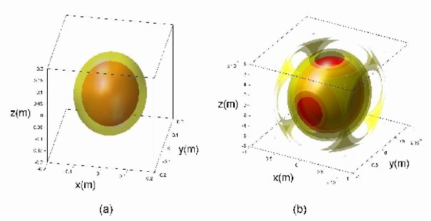
Figure 40: In the previous Figure we have seen how SR, in its non-restricted version (ER), predicted[203, 204] that, while the simplest subluminal object is obviously a sphere (or, in the limit, a space point), the simplest Superluminal object is on the contrary an X-shaped pulse (or, in the limit, a double cone).  The circumstance that the Localized Solutions to the wave equations do follow the same pattern is rather interesting, and is expected to be useful —in the case, e.g., of elementary particles and quantum physics— for a deeper comprehension of de Broglie’s and Schroedinger’s wave mechanics. With regard to the fact that the simplest subluminal LWs, solutions to the wave equations, are “ball-like”, let us depict by these figures, in the ordinary 3D space, the general shape of the Mackinnon’s solutions as expressed by eq.(124), numerically evaluated for $v<<c$. In figures (a) and (b) we graphically represent the field iso-intensity surfaces, which in the considered case result to be (as expected) just spherical.

We have also seen, among the others, that, even if our first method (Section 12) cannot directly yield zero-speed envelopes, such envelopes “at rest”, eq.(145), can be however obtained by applying a $v$-speed LT to eq.(130). In this way, one starts from many frequencies [eq.(130)] and ends up with one frequency only [eq.(145)], since $b$ gets transformed into the frequency of the monochromatic beam.

16 Non-axially symmetric solutions: The case of higher-order Bessel beams

Let us stress that till now we paid attention to exact solutions representing axially-symmetric (subluminal) pulses only: that is to say, to pulses obtained by suitable superpositions of zero-order Bessel beams.

It is however interesting to look also for analytic solutions representing non-axially symmetric subluminal pulses, which can be constructed in terms of superpositions of $\nu$-order Bessel beams, with $\nu$ a positive integer ($\nu>0$).  This can be attempted both in the case of Sect.12 (first method), and in the case of Sect.13 (second method).

For brevity’s sake, let us take only the first method (Sect.12) into consideration.  One is immediately confronted with the difficulty that no exact solutions are known for the integral in eq.(122) when $J_{0}(.)$ is replaced with $J_{\nu}(.)$.

One can overcome this difficulty by following a simple method, which allows obtaining “higher-order” subluminal waves in terms of the axially-symmetric ones.  Indeed, it is well-known that, if $\Psi(x,y,z,t)$ is an exact solution to the ordinary wave equation, then  $\partial\Psi/\partial x$  and  $\partial\Psi/\partial y$  are also exact solutions.^∙  By contrast, when working in cylindrical co-ordinates, if $\Psi(\rho,\phi,z,t)$ is a solution to the wave equation, quantities $\partial\Psi/\partial\rho$  and  $\partial\Psi/\partial\phi$ are not solutions, in general.  Nevertheless, it is not difficult at all to reach the noticeable conclusion that, once  $\Psi(\rho,\phi,z,t)$  is a solution, then also

$$\overline{\Psi}(\rho,\phi,z,t)\;=\;e^{i\phi}\left(\frac{\partial\Psi}{\partial\rho}+\frac{i}{\rho}\frac{\partial\Psi}{\partial\phi}\right)$$ (161)

is an exact solution! For instance, for an axially-symmetric solution of the type $\Psi=J_{0}(k_{\rho}\rho)\,\exp[ik_{z}]\,\exp[-i\omega t]$, equation (161) yields $\overline{\Psi}=-k_{\rho}\,J_{1}(k_{\rho}\rho)\,\exp[i\phi]\,\exp[ik_{z}]\,\exp[-i\omega t]$, which is actually one more analytic solution.

In other words, it is enough to start for simplicity from a zero-order Bessel beam, and to apply eq.(161), successively, $\nu$ times, in order to get as a new solution  $\overline{\Psi}=(-k_{\rho})^{\nu}\,J_{\nu}(k_{\rho}\rho)\,\exp[i\nu\phi]\,\exp[ik_{z}]\,\exp[-i\omega t]$,  which is a $\nu$-order Bessel beam.

In such a way, when applying $\nu$ times eq.(161) to the (axially-symmetric) subluminal solution $\Psi(\rho,z,t)$ in Eqs.(130,129,128)  [obtained from eq.(117) with spectral function $S(\omega)$], we get the subluminal non-axially symmetric pulses  $\Psi_{\nu}(\rho,\phi,z,t)$  as new analytic solutions, consisting as expected in superpositions of $\nu$-order Bessel beams:

$$\Psi_{n}(\rho,\phi,z,t)\;=\;\int_{\omega_{-}}^{\omega_{+}}{\rm d}\omega\;S^{\prime}(\omega)\;J_{\nu}(k_{\rho}\rho)\;e^{i\nu\phi}\;e^{ik_{z}z}\;e^{-i\omega t}\;,$$ (162)

where $k_{\rho}(\omega)$ is given by eq.(118), and quantities $S^{\prime}(\omega)=(-k_{\rho}(\omega))^{\nu}S(\omega)$ are the spectra of the new pulses.  If $S(\omega)$ is centered at a certain carrier frequency (it is a gaussian spectrum, for instance), then $S^{\prime}(\omega)$ too will approximately result to be of the same type.

Now, if we wish the new solution $\Psi_{\nu}(\rho,\phi,z,t)$ to possess a pre-defined spectrum $S^{\prime}(\omega)=F(\omega)$, we can first take eq.(117) and put  $S(\omega)=F(\omega)/(-k_{\rho}(\omega))^{\nu}$  in its solution (130), and afterwards apply to it, $\nu$ times, the operator  $U\equiv\exp[i\phi]\;[\partial/\partial\rho+(i/\rho)\partial/\partial\phi)]\,$:  As a result, we will obtain the desired pulse, $\Psi_{\nu}(\rho,\phi,z,t)$, endowed with $S^{\prime}(\omega)=F(\omega)$.

An example:

On starting from the subluminal axially-symmetric pulse $\Psi(\rho,z,t)$, given by eq.(130) with the gaussian spectrum (131), we can get the subluminal, non-axially symmetric, exact solution $\Psi_{1}(\rho,\phi,z,t)$ by simply calculating

$$\Psi_{1}(\rho,\phi,z,t)\;=\;{{\partial\Psi}\over{\partial\rho}}\ \;e^{i\phi}\;,$$ (163)

which actually yields the “first-order” pulse $\Psi_{1}(\rho,\phi,z,t)$, which can be more compactly written in the form:

$$\Psi_{1}(\rho,\phi,\eta,\zeta)\;=\;2\,{b\over c}\,v\,\gamma^{2}\;{\exp{\left[i{b\over c}\,\beta\,\gamma^{2}\;\eta\right]}}\sum_{n=-\infty}^{\infty}\;A_{n}\;\exp{[in{\pi\over\beta}]}\ \;\psi_{1n}$$ (164)

with

$$\psi_{1n}(\rho,\phi,\eta,\zeta)\equiv\displaystyle{{b^{2}\over c^{2}}\,\gamma^{2}\rho\ \;Z^{-3}\ [Z\,\cos Z-\sin Z]\ \;e^{i\phi}}\;,$$ (165)

where

$$Z\equiv\displaystyle{\sqrt{{b^{2}\over c^{2}}\,\gamma^{2}\rho^{2}+\left({b\over c}\,\gamma^{2}\zeta+n\pi\right)^{2}}}\;.$$ (166)

This exact solution, let us repeat, corresponds to superposition (162),  with  $S^{\prime}(\omega)=k_{\rho}(\omega)S(\omega)$,  quantity $S(\omega)$ being given by eq.(131).  It is represented in Figure 41. The pulse intensity has a “donut-like” shape.

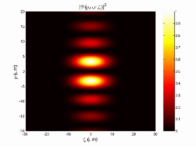
Figure 41: Orthogonal projection of the field intensity corresponding to the higher order subluminal pulse represented by the exact solution eq.(163), quantity $\Psi$ being given by eq.(128) with the gaussian spectrum (131). The pulse intensity happens to have this time a “donut”-like shape.

16.1 A few concluding remarks about the Third Part

In this Third Part we started developing, by suitable superpositions of equal-frequency Bessel beams, a first theoretical and experimental methodology to obtain localized stationary wave fields, with high transverse localization, whose longitudinal intensity pattern can approximately assume any desired shape within a chosen interval $0\leq z\leq L$ of the propagation axis $z$. Their intensity envelope remains static, i.e., with velocity $v=0$;  so that we named “Frozen Waves” (FW) these new solutions to the wave equations (and, in particular, to the Maxwell equations). Inside the envelope of a FW only the carrier wave does propagate: And the longitudinal shape, within the interval $0\leq z\leq L$, can be chosen in such a way that no nonnegligible field exists outside the pre-determined region (consisting, e.g., in one or more high intensity peaks). Such solutions are noticeable also for the different and interesting applications they can have, especially in electromagnetism and acoustics, such as optical tweezers, atom guides, optical or acoustic bistouries, various important medical apparatus (mainly for destroying cancerous cells), etc.

Afterwards, we have addressed the more general subject of the subluminal Localized Waves, and shown that —like in the well-known Superluminal case[143]— the subluminal solutions can be obtained by superposing Bessel beams[141]. Such solutions have been scarcely considered in the past, for the reason that the superposition integral has to run in this case over a finite interval (which makes mathematically difficult to work out analytic expressions for them).  We have shown, however, how it is possible to obtain, in a simple way, non-diffracting subluminal pulses as exact analytic solutions to the wave equations: For arbitrarily chosen frequencies and bandwidths, and avoiding any recourse to the backward-travelling components.

Indeed, till recent times only one closed-form subluminal LW solution, $\psi_{\rm cf}$, to the wave equations was known[151]: obtained by choosing in the relevant integration a constant weight-function $S(\omega)$; whilst all other solutions had been previously got only by numerical simulations. On the contrary, a subluminal LW can be obtained in closed form by adopting, for instance, any spectra $S(\omega)$ that be expansions in terms of $\psi_{\rm cf}$.  In fact, the initial disadvantage, of having to deal with a limited bandwidth, may be turned into an advantage, since in the case of “truncated” integrals the spectrum $S(\omega)$ can be expanded in a Fourier series.  More in general, it has been shown how can one arrive at exact solutions both by integration over the Bessel beams’ angular frequency $\omega$, and by integration over their longitudinal wavenumber $k_{z}$. Both methods have been expounded above. The first one appears to be comprehensive enough; we have studied the second method as well, however, since it furnishes a new way, in terms of continuous spectra, for tackling also the limiting case of zero-speed solutions (i.e., for obtaining the Frozen Waves).

We have briefly treated the case, moreover, of non axially-symmetric solutions, that is, of higher order Bessel beams.

At last, some attention has been paid to the role of Special Relativity, and to the fact that the localized waves are expected to be transformable one into the other by suitable Lorentz Transformations.  Moreover, our results seem to show that in the subluminal case the simplest LW solutions are (for $v<<c$) “ball”-like, as expected since long[203] on the mere basis of special relativity[204].  [Indeed, let us recall once more that already in the years 1980-82 it had been predicted that, if the simplest subluminal object is a sphere (or, in the limit, a space point), then the simplest Superluminal object is an X-shaped pulse (or, in the limit, a double-cone); and viceversa: Cf. Figs.11. It is rather interesting that the same pattern appears to be followed by the localized solutions of the wave equations]. For the subluminal case, see, e.g., Figs.40.

The subluminal localized pulses, endowed with a finite energy, or merely truncated, will be presented elsewhere.

Acknowledgements

The authors are very grateful to Peter Hawkes for his kind invitation to write this paper and encouragement, and to H.E.Hernández-Figueroa for his continuous help and collaboration over the years.  For useful discussions they wish to thank, among the others, also I.M.Besieris, R.Bonifacio, R.Chiao, C.Cocca, C.Conti, A.Friberg, F.Fontana, M.Ibison, G.Kurizki, I.Licata, J-y.Lu, A.Loredo, M.Mattiuzzi, P.Milonni, S.Narayana, P.Nelli, P.Saari, A.M.Shaarawi, E.C.G.Sudarshan, M.Tygel, and R.Ziolkowski.  Finally, thanks are due to M. Tenório de Vasconselos and J. Marchi Madureira for their willingness and patient cooperation.

References

- [1] M.Born and E.Wolf: Principles of Optics — Electromagnetic Theory of Propagation, Interference and Diffraction of Light, 6th edition (Cambridge Univ. Press; Cambridge, 1998).
- [2] H.A.Willebrand and B.S.Ghuman: “Fiber Optics Without Fiber”, IEEE Spectrum, vol.38, no.8 (2001).
- [3] J.W.Goodman: Introduction to Fourier Optics, 2nd edition (McGraw-Hill; New York, 1996).
- [4] S.Okazaki: “Resolution limits of optical lithography”, Journal of Vacuum Science and Technology B, vol.9, pp.2829-2833 (1991).
- [5] T.Ito and S.Okazaki: “Pushing the limits of lithography”, Nature, vol.406, pp.1027-1031 (2000).
- [6] A.Ashkin, J.M.Dziedzic, J.E.Bjorkholm and S.Chu: “Observation of a single-beam gradient force optical trap for dielectric particles”, Optics Letters, vol.11, pp.288-290 (1986).
- [7] J.E.Curtis, B.A.Koss and D.G.Grier: “Dynamic holographic optical tweezers”, Optics Communications, vol.207, pp.169-175 (2002).
- [8] G.P.Agrawal: Nonlinear Fiber Optics, 2nd edition (Acad. Press; New York, 1995).
- [9] A.O.Barut, G.D.Maccarrone and E.Recami: “On the Shape of Tachyons”, Nuovo Cimento A, vol.71, pp.509-533 (1982); and refs. therein. Cf. also E.Recami and G.D.Maccarrone: Lett. Nuovo Cim. 28 (1980) 151-157 ; ibidem, 37 (1983) 345-352; P.Caldirola, G.D.Maccarrone and E.Recami: Lett. Nuovo Cim. 29 (1980) 241-250; G.D.Maccarrone, M.Pavsic and E.Recami: Nuovo Cimento B73 (1983) 91-111.
- [10] J.A.Stratton: Electromagnetic Theory, page 356 (McGraw-Hill; New York, 1941).
- [11] R.Courant and D.Hilbert: Methods of Mathematical Physics, vol.2, p.760 (J.Wiley; New York, 1966).
- [12] H.Bateman: Electrical and Optical Wave Motion (Cambridge Univ.Press; Cambridge, 1915).
- [13] E.Recami, M.Zamboni-Rached and C.A.Dartora: “The X-shaped, localized field generated by a Superluminal electric charge” [e-print physics/0210047], Physical Review E, vol.69, no.027602 (2004) [4 pages].
- [14] J.-y. Lu and J.F.Greenleaf: “Nondiffracting X-waves: Exact solutions to free-space scalar wave equation and their finite aperture realizations”, IEEE Transactions in Ultrasonics Ferroelectricity and Frequency Control, vol.39, pp.19-31 (1992); and refs. therein.
- [15] J.-y.Lu, J.F.Greenleaf and E.Recami, “Limited diffraction solutions to Maxwell (and Schroedinger) equations” [Lanl Archives e-print physics/9610012], Report INFN/FM–96/01 (I.N.F.N.; Frascati, Oct.1996); E.Recami: “On localized X-shaped Superluminal solutions to Maxwell equations,” Physica A, vol.252, pp.586-610 (1998); and refs. therein. See also R.W.Ziolkowski, I.M.Besieris and A.M.Shaarawi, J. Opt. Soc. Am., vol.A10, p.75 (1993); J. Phys. A: Math.Gen., vol.33, pp.7227-7254 (2000).
- [16] J.-y. Lu and J.F.Greenleaf: “Experimental verification of nondiffracting X-waves”, IEEE Transactions in Ultrasonics Ferroelectricity and Frequency Control, vol.39, pp.441-446 (1992).
- [17] P.Saari and K.Reivelt: “Evidence of X-shaped propagation-invariant localized light waves,” Physical Review Letters, vol.79, pp.4135-4138 (1997).
- [18] D.Mugnai, A.Ranfagni, and R.Ruggeri: “Observation of Superluminal behaviours in wave propagation,” Physical Review Letters, vol.84, pp.4830-4833 (2000).
- [19] J.-y. Lu, H.-H.Zou and J.F.Greenleaf: “Biomedical ultrasound beam forming”, Ultrasound in Medicine and Biology, vol.20, pp.403-428 (1994).
- [20] J.-y. Lu, H.-h.Zou and J.F.Greenleaf: “Producing deep depth of field and depth independent resolution in NDE with limited diffraction beams”, Ultrasonic Imaging, vol.15, pp.134-149, 1993.
- [21] V.Garcés-Chavez, D.McGloin, H.Melville, W.Sibbett and K.Dholakia: “Simultaneous micromanipulation in multiple planes using a self-reconstructing light beam”, Nature, vol.419, pp.145-147 (2002).
- [22] D.McGloin, V.Garcés-Chavez and K.Dholakia: “Interfering Bessel beams for optical micromanipulation”, Optics Letters, Vol.28, pp.657-659 (2003).
- [23] M.P.MacDonald et al.: “Creation and manipulation of three-dimensional optically trapped structures”, Science, Vol.296, pp.1101-1103 (2002).
- [24] J.Arlt, V.Garcés-Chavez, W.Sibbett and K.Dholakia: “Optical micromanipulation using a Bessel light beam”, Optics Communications, vol.197, pp.239-245 (2001).
- [25] D.P.Rhodes, G.P.T.Lancaster, J.Livesey, D.McGloin, J.Arlt and K.Dholakia: “Guiding a cold atomic beam along a co-propagating and oblique hollow light guide”, Optics Communications, vol.214, pp.247-254 (2002).
- [26] J.Fan, E.Parra and H.M.Milchberg: “Resonant self-trapping and absorption of intense Bessel beams”, Physical Review Letters, vol.84, pp.3085-3088 (2000).
- [27] J.Arlt, T.Hitomi and K.Dholakia: “Atom guiding along Laguerre-Gaussian and Bessel light beams”, Applied Physics B, vol.71, pp.549-554 (2000).
- [28] M.Erdélyi, Z.L.Horvath, G.Szabo, Zs.Bor, F.K.Tittell, J.R.Cavallaro and M.C.Smayling: “Generation of diffraction-free beams for applications in optical Microlithography”, Journal of Vacuum Science and Technology B, vol.15, pp.287-292 (1997), and refs. therein.
- [29] R.M.Herman and T.A.Wiggins: “Production and uses of diffractionless beams,” Journal of the Optical Society of America A, vol.8, pp.932-942 (1991).
- [30] R.W.Ziolkowski: “Localized transmission of electromagnetic energy,” Physical Review A, vol.39, pp.2005-2033 (1989).
- [31] R.W.Ziolkowski: ”Localized wave physics and engineering,” Physical Review A, vol.44, pp.3960-84 (1991).
- [32] J.-y. Lu and H.Shiping: “Optical X wave communications”, Optics Communications, vol.161, pp.187-192 (1999).
- [33] A.Vasara, J.Turunen and A.T.Friberg: “Realization of general nondiffracting beams with computer-generated holograms”, Journal of the Optical Society of America A, vol.6, pp.1748-1754 (1989); J.Salo, J.Fagerholm, A.T.Friberg and M.M.Salomaa, “Nondiffracting bulk-acoustic X-waves in crystals”, Phys. Rev. Lett. 83 (1990) 1171-74; J.Salo, A.T.Friberg and M.M.Salomaa, “Orthogonal X-waves”, J. Phys. A: Math. Gen. 34 (2001) 9319-27.
- [34] E.Recami, M.Zamboni-Rached and H.E.Hernández-Figueroa: “Localized waves: A scientific and historical introduction”, introductory Chapter of the book quoted below in ref.[143].
- [35] See, e.g., A.O.Barut and H.C.Chandola, “Localized tachyonic wavelet solutions of the wave equation”, Physics Letters A, vol.180, pp.5-8 (1993); and refs. therein.
- [36] J.Durnin, J.J.Miceli and J.H.Eberly: “Diffraction-free beams,” Physical Review Letters, vol. 58, pp.1499-1501 (1987).
- [37] J.Durnin: “Exact solutions for nondiffracting beams: I. The scalar theory,” Journal of the Optical Society of America A, vol.4, pp.651-654 (1987).
- [38] M.Zamboni-Rached, E.Recami and H.E.Hernández-Figueroa: “New localized Superluminal solutions to the wave equations with finite total energies and arbitrary frequencies,” European Physical Journal D, vol.21, pp.217-228 (2002).
- [39] Z.Bouchal, J.Wagner and M.Chlup: “Self-reconstruction of a distorted nondiffracting beam”, Optics Communications, vol.151, pp.207-211 (1998).
- [40] M.Zamboni-Rached: private communications (2003).
- [41] R.Grunwald et al., “Generation and characterization of spatially and temporally localized few-cycle optical wavepackets”, Phys. Rev. A67 (2003) 063820; R.Grunwald, U.Griebner, U.Neumann and V.Kebbel, “Self-recontruction of ultrashort-pulse Bessel-like X-waves”, CLEO/QELS Conference (San Francisco; 2004), paper no.CMQ7; R.Grunwald et al., “Ultrabroadband spectral transfer in extended focal zones: truncated few-cycle Bessel-Gauss beams”, CLEO Conference (Baltimore, 2005), paper CTuAA6.
- [42] R.P.MacDonald, J.Chrostowski, S.A.Boothroyd and B.A.Syrett: “Holographic Formation of a Diode Laser Non-Diffracting Beam”, Applied Optics, vol.32, pp.6470-6474 (1983).
- [43] M.Zamboni-Rached: “Stationary optical wave fields with arbitrary longitudinal shape by superposing equal frequency Bessel beams: Frozen Waves”, Optics Express, vol.12, pp.4001-4006 (2004).
- [44] M.Zamboni-Rached, E.Recami and H.E.Hernández-Figueroa: “Theory of ‘Frozen Waves’ [e-print physics/0502105], Journal of the Optical Society of America A, vol.11, pp.2465-2475 (2005).
- [45] M.Zamboni-Rached, “Diffraction-attenuation resistant beams in absorbing media”, Opt. Express 14 (2006) 1804-1809 [paper chosen for mention also in the Virtual Journal for Biomedical Optics, and in Laser Focus World, Section “new bracks”].
- [46] A.O.Barut and A.Grant: “Quantum particle-like configurations of the electromagnetic field”, Found. Phys. Lett., vol.3, pp.303-310 (1990).
- [47] A.O.Barut and A.J.Bracken: “Particle-like configurations of the electromagnetic field: an extension of de Broglie’s ideas”, Found. Phys., vol.22, pp.1267-1285 (1992).
- [48] J.N.Brittingham: “Focus wave modes in homogeneous Maxwell’s equations: transverse electric mode,” J. Appl. Phys., vol.54, pp.1179-1189 (1983).
- [49] A.Sezginer: “A general formulation of focus wave modes”, J. Appl. Phys., vol.57, pp.678-683 (1985).
- [50] I.M.Besieris, A.M.Shaarawi and R.W.Ziolkowski: “A bidirectional travelling plane wave representation of exact solutions of the scalar wave equation”, J. Math. Phys., vol.30, pp.1254-1269 (1989).
- [51] A.M.Shaarawi, I.M.Besieris and R.W.Ziolkowski: “A novel approach to the synthesis of nondispersive wave packet solutions to the Klein-Gordon and Dirac equations”, J. Math. Phys., vol.31, pp.2511-2519 (1990).
- [52] R.W.Ziolkowski, I.M.Besieris and A.M.Shaarawi: “Aperture realizations of exact solutions to homogeneous wave equations”, Journal of the Optical Society of America A, vol.10, pp.75-87 (1993).
- [53] R.Donnelly and R.W.Ziolkowski: “Designing localized waves”, Proceedings of the Royal Society of London, A, vol.440, pp.541-565 (1993).
- [54] E.Recami: “Classical Tachyons and Possible Applications”, Rivista Nuovo Cim. 9(6) (1986) 1–178, issue no.6; and refs. therein.
- [55] E.Recami, M.Zamboni-Rached, K.Z.Nobrega, C.A.Dartora and H.E.Hernández-Figueroa: “On the Localized Superluminal Solutions to the Maxwell Equations”, IEEE Journal of Selected Topics in Quantum Electronics, Vol.9, pp.59-73 (2003).
- [56] E.Recami: “Superluminal motions? A bird’s-eye view of the experimental status-of-the-art”, Found. Phys., vol.31, pp.1119-1135 (2001).
- [57] E.Recami, F.Fontana and R.Garavaglia: “Superluminal motions and Special Relativity: A discussion of recent experiments”, Int. J. Mod. Phys. A, vol.15, pp.2793-2812 (2000). Cf. also R.Garavaglia, Thesis work (Dip. Sc. Informazione, Università statale di Milano; Milan, 1998; G.Degli Antoni and E.Recami supervisors); and M.Pavsic and E.Recami: “Charge Conjugation and Internal Space-Time Symmetries”, Lett. Nuovo Cimento 34 (1982) 357-362.
- [58] E.Recami: “Tachyon Mechanics and Causality; A Systematic Thorough Analysis of the Tachyon Causal Paradoxes”, Foundations of Physics 17 (1987) 239-296. See also E.Recami: “The Tolman-Regge Antitelephone Paradox: Its Solution by Tachyon Mechanics”, Lett. Nuovo Cimento 44 (1985) 587-593; and G.D.Maccarrone and E.Recami: “Two-Body Interactions through Tachyon Exchange”, Nuovo Cimento A57 (1980) 85-101.
- [59] A.T.Friberg, J.Fagerholm and M.M.Salomaa: “Space-frequency analysis of nondiffracting pulses”, Optics Communications, vol.136, pp.207-212 (1997).
- [60] R.W.Ziolkowski, I.M.Besieris and A.M.Shaarawi: “Aperture realizations of exact solutions to homogeneous wave equations”, Journal of the Optical Society of America A, vol.10, pp.75-87 (1993).
- [61] A.M.Shaarawi and I.M.Besieris: “On the Superluminal propagation of X-shaped localized waves”, J. Phys. A, vol.33, pp.7227-7254 (2000).
- [62] A.M.Shaarawi and I.M.Besieris: “Relativistic causality and Superluminal signalling using X-shaped localized waves”, J. Phys. A, vol.33, pp.7255-7263, 2000; and refs. therein.
- [63] A.P.L.Barbero, H.E.Hernández F., and E.Recami, “On the propagation speed of evanescent modes”, Phys. Rev. E, vol.62, p.8628 (2000), and refs. therein. Cf. also A.M.Shaarawi and I.M.Besieris, Phys. Rev. E, vol.62, p.7415 (2000).
- [64] H.M.Brodowsky, W.Heitmann and G.Nimtz, Phys. Lett. A, vol.222, p.125 (1996).
- [65] W.Ziolkowski, I.M.Besieris and A.M.Shaarawi: “Aperture realizations of exact solutions to homogeneous wave-equations”, J. Opt. Soc. Am., vol.A10 (1993) 75, Sects.5 and 6.
- [66] See M.Zamboni-Rached: “Localized solutions: Structure and Applications”, M.Sc. Thesis, 1999, Universidade Estadual de Campinas, Phys.Dept. (supervised by H.E.H.Figueroa and E.Recami); M.Zamboni-Rached, “Localized waves in diffractive/dispersive media”, PhD Thesis, Aug.2004, Universidade Estadual de Campinas, DMO/FEEC (supervised by H.E.H.Figueroa).
- [67] A.C.Newell and J.V.Molone, Nonlinear Optics (Addison & Wesley; Redwood City, CA, 1992).
- [68] M.Zamboni-Rached, H.E.Hernández-Figueroa and E.Recami: “Chirped optical X-shaped pulses in material media”, J. Opt. Soc. Am. A21 (2004) 2455-2463.
- [69] J.Durnin, J.J.Miceli and J.H.Eberly: “Comparison of Bessel and Gaussian beams”, Optics Letters, vol.13, pp.79-80 (1988).
- [70] P.L.Overfelt and C.S.Kenney: “Comparison of the propagation characteristics of Bessel, Bessel-Gauss, and gaussian beams diffracted by a circular aperture”, Journal of the Optical Society of America A, vol.8, pp.732-745 (1991).
- [71] C.A.Dartora, M.Zamboni-Rached, K.Z.Nobrega, E.Recami and H.E.Hernández-Figueroa: “General formulation for the analysis of scalar diffraction-free beams using angular modulation: Mathieu and Bessel Beams”, Optics Communications, vol.222, pp.75-80 (2003).
- [72] Ettore Majorana - Notes on Theoretical Physics, edited by S.Esposito, E.Majorana jr., A. van der Merwe and E.Recami (Kluwer; Dordrecht and N.Y., Nov.2003), 512 pages.
- [73] M.Zamboni-Rached, E.Recami and F.Fontana: “Localized Superluminal solutions to Maxwell equations propagating along a normal-sized waveguide,” Physical Review E, vol.64, no.066603 (2001) [6 pages]. See also “Superluminal localized solutions to Maxwell equations propagating along a waveguide: The finite-energy case,” Phys. Rev.E, vol.67, no.036620 (2003) [7 pages].
- [74] F.Selleri, talk presented at the “2nd Cracow-Clausthal workshop on Extensions of quantum theory”, Krakow, 2000 (unpublished); and in F.Selleri, “Lezioni di relatività da Einstein all’etere di Lorentz” (Progedit pub.; Bari, 2003).
- [75] C.Conti, S.Trillo, G.Valiulis, A.Piskarkas, O. van Jedrkiewicz, J.Trull and P.Di Trapani, “Non-linear electromagnetic X-waves”, Phys. Rev. Lett. 90 (2003) 170406.
- [76] See, e.g., O.M.Bilaniuk, V.K.Deshpande and E.C.G.Sudarshan, Am. J. Phys., vol.30, 718 (1962).
- [77] E.Recami and R.Mignani: Rivista Nuovo Cim. 4 (1974) 209-290, E398.
- [78] See, e.g., E.Recami (editor): Tachyons, Monopoles, and Related Topics (North-Holland; Amsterdam; 1978), pp.X + 285.
- [79] M. Zamboni-Rached, “Analytical expressions for the longitudinal evolution of nondiffracting pulses truncated by finite apertures,” J. Opt. Soc. Am. A 23 (2006) 2166-2176.
- [80] See E.Recami: ref.[54], pp.80-81; and figure 27 and refs. therein; and R.Folman and E.Recami: Found. Phys. Lett. 8 (1995) 127-134.
- [81] I.S.Gradshteyn and I.M.Ryzhik: Integrals, Series and Products, 4th edition (Ac.Press; New York, 1965).
- [82] M.Zamboni-Rached, K.Z.Nobrega, H.E.Hernández-Figueroa and E.Recami: “Localized Superluminal solutions to the wave equation in (vacuum or) dispersive media, for arbitrary frequencies and with adjustable bandwidth”, Optics Communications, vol.226, pp.15-23 (2003).
- [83] E.Recami and R.Mignani: “Magnetic Monopoles and Tachyons in Special Relativity”, Physics Letters B62 (1976) 41-43.
- [84] M.Zamboni-Rached and E.Recami: “Cherenkov radiation has nothing to do with X-shaped Localized Waves (Comments on ‘Cherenkv-Vavilov formulation of X-waves’)”, e-print arXiv:0807.4301v2[physics.Optics], 19 Aug. 2008.
- [85] Cf. M.Baldo Ceolin, “Review of neutrino physics”, invited talk at the XXIII Int. Symp. on Multiparticle Dynamics (Aspen, CO; Sept.1993); E.W.Otten, Nucl. Phys. News, vol.5, 11 (1995). From the theoretical point of view, see, e.g., E.Giannetto et al., ref.[86] and refs. therein; S.Giani, “Experimental evidence of Superluminal velocities in astrophysics and proposed experiments”, CP458, in Space Technology and Applications International Forum 1999, ed. by M.S.El-Genk (A.I.P.; Melville, 1999), pp.881-888.
- [86] E.Giannetto, G.D.Maccarrone, R.Mignani and E.Recami, Phys. Lett. B178 (1986) 115-120 (1986) and refs. therein.
- [87] See, e.g., J.A.Zensus and T.J.Pearson (editors), Superluminal Radio Sources (Cambridge Univ.Press; Cambridge, UK, 1987).
- [88] I.F.Mirabel and L.F.Rodriguez, “A Superluminal source in the Galaxy”, Nature, vol.371, 46 (1994) [with an editorial comment, “A galactic speed record”, by G.Gisler, at page 18 of the same issue]; S.J.Tingay et al., “Relativistic motion in a nearby bright X-ray source”, Nature, vol.374, 141 (1995).
- [89] M.J.Rees, Nature, vol.211, 46 (1966); A.Cavaliere, P.Morrison and L.Sartori, Science, vol.173, 525 (1971).
- [90] E.Recami, A.Castellino, G.D.Maccarrone and M.Rodonò, “Considerations about the apparent Superluminal expansions observed in astrophysics”, Nuovo Cimento B93, 119 (1986). Cf. also R.Mignani and E.Recami, Gen. Relat. Grav., 5 (1974) 615.
- [91] V.S.Olkhovsky and E.Recami, “Recent Developments in the Time Analysis of Tunnelling Processes”, Physics Reports 214 (1992) 339-357, issue n 6, and refs. therein: In particular T.E.Hartman, J. Appl. Phys., vol.33, p.3427 (1962); L.A.MacColl, Phys. Rev., vol.40 (1932) 621. See also V.S.Olkhovsky, E.Recami, F.Raciti and A.K.Zaichenko, J. de Physique-I, vol.5, 1351-1365 (1995); V.S.Olkhovsky, E.Recami and J.Jakiel, “Unified time analysis of photon and nonrelativistic particle tunnelling” [Report INFN/FM-01/01 (Infn; Frascati, Apr.2001)], e-print quant-ph/0102007; P.W.Milonni, J. Phys. B, vol.35 (2002) pp.R31-R56.
- [92] V.S.Olkhovsky, E.Recami, F.Raciti and A.K.Zaichenko, J. de Phys.-I, vol.5, 1351-1365 (1995).
- [93] V.S.Olkhovsky, E.Recami and J.Jakiel, “Unified time analysis of photon and nonrelativistic particle tunnelling”, Physics Reports 398 (2004) 133-178.
- [94] V.S.Olkhovsky, E.Recami and A.K.Zaichenko: “Resonant and non-resonant tunnelling through a double barrier”, Europhysics Letters 70 (2005) 712-718.
- [95] See, e.g., R.Y.Chiao, P.G.Kwiat and A.M.Steinberg, Physica B, vol.175, 257 (1991); A.Ranfagni, D.Mugnai, P.Fabeni and G.P.Pazzi, Appl. Phys. Lett., vol.58, 774 (1991); Th.Martin and R.Landauer, Phys. Rev. A, vol.45, 2611 (1992); Y.Japha and G.Kurizki, Phys. Rev. A, vol.53, 586 (1996). Cf. also G.Kurizki, A.E.Kozhekin and A.G.Kofman, Europhys. Lett., vol.42, 499 (1998); G.Kurizki, A.E.Kozhekin, A.G.Kofman and M.Blaauboer, paper delivered at the VII Seminar on Quantum Optics, Raubichi, BELARUS (May, 1998).
- [96] G.Nimtz and A.Enders, J. de Physique-I, vol.2, 1693 (1992); vol.3, 1089 (1993); vol.4, 1379 (1994); Phys. Rev. E, vol.48, 632 (1993); H.M.Brodowsky, W.Heitmann and G.Nimtz, J. de Physique-I, vol.4, 565 (1994); Phys. Lett. A, vol.222, 125 (1996); vol.196, 154 (1994). For a review, see, e.g., G.Nimtz and W.Heitmann, Prog. Quant. Electr., vol.21, 81 (1997).
- [97] A.M.Steinberg, P.G.Kwiat and R.Y.Chiao, Phys. Rev. Lett., vol.71, 708 (1993), and refs. therein; Scient. Am., vol.269(2), p.38 (1993), issue no.2. For a review, see, e.g., R.Y.Chiao and A.M.Steinberg, in Progress in Optics, ed. by E.Wolf (Elsevier; Amsterdam, 1997), p.345. Cf. also Y.Japha and G.Kurizki, Phys. Rev. A, vol.53, p.586 (1996).
- [98] A.Ranfagni, P.Fabeni, G.P.Pazzi and D.Mugnai, Phys. Rev. E, vol.48, p.1453 (1993); Ch.Spielmann, R.Szipocs, A.Stingl and F.Krausz, Phys. Rev. Lett., vol.73, p.2308 (1994), Ph.Balcou and L.Dutriaux, Phys. Rev. Lett., vol.78, p.851 (1997); V.Laude and P.Tournois, J. Opt. Soc. Am., vol.B16, p.194 (1999).
- [99] Scientific American (Aug. 1993); Nature (Oct.21, 1993); New Scientist (Apr. 1995); Newsweek (19 June 1995).
- [100] Ref.[54], p.158 and pp.116-117. Cf. also D.Mugnai, A.Ranfagni, R.Ruggeri, A.Agresti and E.Recami, Phys. Lett. A, vol.209, 227 (1995).
- [101] See, for instance, P.W.Milonni, J. Phys. B, vol.35 (2002) R31-R56; G.Nimtz and A.Haibel, Ann. der Phys., vol.11 (2002) 163-171; R.W.Ziolkowski, Phys. Rev. E, vol.63 (2001) 046604; A.M.Shaarawi and I.M.Besieris, J. Phys. A, vol.33 (2000) 7227-7254; 7255-7263; E.Recami, F.Fontana and R.Garavaglia, ref.[57] and refs. therein
- [102] S.Longhi, P.Laporta, M.Belmonte and E.Recami: “Measurement of Superluminal optical tunnelling times in double-barrier photonic bandgaps”, Phys. Rev. E, vol.65 (2002) 046610.
- [103] L.J.Wang, A.Kuzmich and A.Dogariu, Nature, vol.406 (2000) 277.
- [104] G.Nimtz, A.Enders and H.Spieker, in Wave and Particle in Light and Matter, ed. by A.van der Merwe and A.Garuccio (Plenum; New York, 1993); J. de Physique-I, vol.4, 565 (1994). See also A.Enders and G.Nimtz, Phys. Rev. B, vol.47, 9605 (1993).
- [105] V.S.Olkhovsky, E.Recami and G.Salesi, Europhysics Letters 57 (2002) 879-884; “Tunneling through two successive barriers and the Hartman (Superluminal) effect”, LANL archives e-print quant-ph/0002022; Y.Aharonov, N.Erez and B.Reznik, Phys. Rev. A, vol.65 (2002) 052124; S.Esposito: Phys. Rev. E67 (2003) 016609. Cf. also E.Recami: “Superluminal tunnelling through successive barriers: Does quantum mechanics predict infinite group velocities?”, J. Mod. Optics 51 (2004) 913-923.
- [106] E.Recami: “Superluminal motions? A bird-eye view of the experimental situation”, Found. Phys. 31 (2001) 1119-1135; V.S.Olkhovsky, E.Recami and G.Salesi: “Tunneling through two successive barriers and the Hartman (Superluminal) effect”, Lanl archives e-print quant-ph/0002022]; Europhys. Lett. 57 (2002) 879-884. Cf. also E.Recami, M.Z.Rached, K.Z.Nobrega, C.A.Dartora and H.E.Hernandez F.: ”On the localized Superluminal solutions to the Maxwell equations”, IEEE Journal of Selected Topics in Quantum Electronics 9(1) (2003) 59-73; E.Recami: “Superluminal tunnelling through successive barriers: Does quantum mechanics predict infinite group velocities?”, J. Mod. Optics 51 (2004) 913-923.
- [107] V.S.Olkhovsky, E.Recami, F.Raciti and A.K.Zaichenko, ref.[ref[12]], page 1361 and refs. therein; E.Recami, F.Fontana and R.Garavaglia, ref.[81], page 2807; and ref.[93], page 152.
- [108] V.Petrillo and L.Refaldi: Phys. Rev. A67 (2003) 012110; V.Petrillo and L.Refaldi: Opt. Commun. 186 (2000) 35. See also L.Refaldi: MSc thesis (V.Petrillo, R.Bonifacio, E.Recami supervisors), Phys. Dept., Milan Univ., 2000.
- [109] R.Y.Chiao, A.E.Kozhekin A.E., and G.Kurizki, Phys. Rev. Lett., vol.77, 1254 (1996); E.L.Bolda et al., Phys. Rev. A, vol.48 (1993) 3890; C.G.B.Garrett and D.E.McCumber, Phys. Rev. A, vol.1, 305 (1970).
- [110] S.Chu and Wong W., Phys. Rev. Lett., vol.48 (1982) 738; B.Segard and B.Macke, Phys. Lett. A, vol.109 (1985) 213-216; B.Macke et al., J. Physique, vol.48 (1987) 797-808; M.W.Mitchell and R.Y.Chiao, Phys. Lett. A, vol.230 (1997) 133-138; L.J.Wang, A.Kuzmich and A.Dogariu, Nature, vol.406 (2000) 277; G.Nimtz, Europ. Phys. J., B, vol.7, 523-525 (1999).
- [111] G.Alzetta, A.Gozzini, L.Moi and G.Orriols: Nuovo Cimento B, vol.36, 5 (1976).
- [112] M.Artoni, G.C.La Rocca, F.S.Cataliotti and F.Bassani: Phys. Rev. A, vol.63, no.023805 (2001).
- [113] M.Zamboni-Rached, K.Z.Nobrega, E.Recami and H.E.Hernández-Figueroa: “Superluminal X-shaped beams propagating without distortion along a coaxial guide,” Physical Review, vol.E66, no.036620 (2002) [10 pages]; and refs. therein.
- [114] M.Zamboni-Rached, E.Recami and H.E.Hernández-Figueroa: “Structure of the nondiffracting waves, and some interesting applications”, a Chapter of the book quoted below in ref.[143].
- [115] See also the large lists of references contained in the book Localized waves, edited by H.E.Hernández-Figueroa, M.Zamboni-Rached and Erasmo Recami (J.Wiley; New York, Jan.2008).
- [116] J. N. Brittingham, “Focus wave modes in homogeneous Maxwell’s equations: transverse electric mode,” J. Appl. Phys., Vol. 54, pp. 1179-1189 (1983).
- [117] J. Durnin, J. J. Miceli e J. H. Eberly, “Diffraction-free beams,” Phys. Rev. Lett., Vol. 58, pp. 1499-1501 (1987).
- [118] J.-y. Lu, J. F. Greenleaf, “Nondiffracting X-waves - Exact solutions to free-space wave equation and their finite aperture realizations,” IEEE Transactions in Ultrasonics Ferroelectricity and Frequency Control, Vol.39, pp.19-31 (1992); and refs. therein.
- [119] H.Sõnajalg, P.Saari, “Suppression of temporal spread of ultrashort pulses in dispersive media by Bessel beam generators”, Opt. Letters, Vol. 21, pp.1162-1164 (1996).
- [120] M. Zamboni-Rached, K. Z. Nóbrega, H. E. Hern\a’ndez-Figueroa e E. Recami, “Localized Superluminal solutions to the wave equation in (vacuum or) dispersive media, for arbitrary frequencies and with adjustable bandwidth”, Optics Communications, Vol.226, pp. 15-23 (2003).
- [121] M.A.Porras, R.Borghi, and M.Santarsiero, “Suppression of dispersion broadening of light pulses with Bessel-Gauss beams”, Optics Communications, Vol. 206, 235-241 (2003).
- [122] C.Conti, S.Trillo, P.Di Trapani, G.Valiulis, A.Piskarskas, O.Jedrkiewicz and J.Trull, “Nonlinear electromagnetic X-waves”, Phys. Rev. Lett., vol.90, paper no.170406, May 2003; and refs. therein.
- [123] J. Salo, J. Fagerholm, A. T. Friberg, and M. M. Salomaa, “Nondiffracting Bulk-Acoustic X waves in Crystals,” Phys. Rev. Lett., Vol. 83, pp. 1171-1174 (1999); and refs. therein.
- [124] M. Zamboni-Rached, ”Diffraction-Attenuation resistant beams in absorbing media”, Optics Express, Vol. 14, pp.1804-1809 (2006).
- [125] I. M. Besieris, A. M. Shaarawi e R. W. Ziolkowski, “A bidirectional travelling plane wave representation of exact solutions of the scalar wave equation”, J. Math. Phys., Vol. 30, pp. 1254-1269 (1989).
- [126] M. Zamboni-Rached, “ Localized Waves: Structure and Applications,” M.Sc. Thesis (Physics Department, Unicamp, 1999).
- [127] M. Zamboni-Rached, E. Recami, H. E. Hernández-Figueroa, ”New localized Superluminal solutions to the wave equations-with finite total energies and arbitrary frequencies”, European Physics Journal D, Vol. 21, 217-228 (2002).
- [128] M.Zamboni-Rached, “Localized waves in diffractive/dispersive media”, PhD Thesis, Aug.2004, Universidade Estadual de Campinas, DMO/FEEC. Download at: http://libdigi.unicamp.br/document/?code=vtls000337794
- [129] S. Longhi, “Localized subluminal envelope pulses in dispersive media,” Optics Letters, Vol. 29, pp.147-149 (2004);and refs. therein.
- [130] M. Zamboni-Rached, “Stationary optical wave fields with arbitrary longitudinal shape by superposing equal frequency Bessel beams: Frozen Waves”, Optics Express, Vol. 12, pp.4001-4006 (2004).
- [131] M. Zamboni-Rached, E. Recami, H. E. Hernández-Figueroa, “Theory of Frozen Waves: Modelling the Shape of Stationary Wave Fields”, Journal of Optical Society of America A, Vol. 22, pp.2465-2475.
- [132] S. V. Kukhlevsky and M. Mechler, “Diffraction-free subwavelength-beam optics at nanometer scale,” Optics Communications, Vol. 231, pp.35-43 (2004).
- [133] I.S.Gradshteyn, and I.M.Ryzhik: Integrals, Series and Products, 4th edition (Acad. Press; New York, 1965).
- [134] A.M.Shaarawi, I.M.Besieris and T.M.Said, “Temporal focusing by use of composite X-waves”, J. Opt. Soc. Am., A, vol.20, pp.1658-1665, Aug.2003.
- [135] M. Zamboni-Rached, A. Shaarawi, E. Recami, “Focused X-Shaped Pulses”, Journal of Optical Society of America A, Vol. 21, pp. 1564-1574 (2004).
- [136] M. Zamboni-Rached, H.E. Hernández-Figueroa, E. Recami “Chirped Optical X-type Pulses,” Journal of Optical Society of America A, Vol. 21, pp. 2455-2463 (2004).
- [137] G. Agrawal: Nonlinear Fiber Optics (Academic Press; 4th edition, 2006).
- [138] Z. Bouchal and M. Olivik, “Non-diffractive vector Bessel beams,” Journal of Modern Optics, Vol. 42, pp.1555-1566 (1995).
- [139] E.Recami: “On localized X-shaped Superluminal solutions to Maxwell equations,” Physica A, Vol. 252, pp.586-610 (1998).
- [140] Z. Bouchal, “Controlled spatial shaping of nondiffracting patterns and arrays”, Optics Letters, Vol. 27, pp. 1376-1378 (2002).
- [141] M.Zamboni-Rached and Erasmo Recami: “Subluminal wave bullets: Exact subluminal localized solutions to the wave equations” [e-print arXix:0709.2372], Physical Review A77 (2008) 033824.
- [142] R. Grunwald, U. Griebner, U. Neumann, and V. Kebbel, “Self-reconstruction of ultrashort-pulse Bessel-like X-waves”, CLEO / QELS 2004, San Francisco, May 16-21, 2004, Conference Digest (CD-ROM), paper number CMQ7.
- [143] Localized Waves, ed. by H.E.Hernández-Figueroa, M.Zamboni-Rached, and E.Recami (J.Wiley; New York, Jan.2008).
- [144] J.-y. Lu and J.F.Greenleaf: “Nondiffracting X-waves: Exact solutions to free-space scalar wave equation and their finite aperture realizations”, IEEE Transactions in Ultrasonics Ferroelectricity and Frequency Control 39 (1992) 19-31; and refs. therein.
- [145] M.Zamboni-Rached, E.Recami and H.E.Hernández-Figueroa: “New localized Superluminal solutions to the wave equations with finite total energies and arbitrary frequencies”, European Physical Journal D21 (2002) 217-228.
- [146] E.Recami, M.Zamboni-Rached, K.Z.Nobrega, C.A.Dartora and H.E.Hernández-Figueroa: “On the Localized Superluminal Solutions to the Maxwell Equations”, IEEE Journal of Selected Topics in Quantum Electronics 9 (2003) 59-73.
- [147] J.-y. Lu and J.F.Greenleaf: “Experimental verification of nondiffracting X-waves”, IEEE Transactions in Ultrasonics Ferroelectricity and Frequency Control 39 (1992) 441-446.
- [148] E.Recami: “On localized X-shaped Superluminal solutions to Maxwell equations”, Physica A252 (1998) 586-610; and refs. therein.
- [149] H.Bateman: Electrical and Optical Wave Motion (Cambridge Univ.Press; Cambridge, 1915).
- [150] R.Courant and D.Hilbert: Methods of Mathematical Physics, vol.2, p.760 (J.Wiley; New York, 1966).
- [151] L. Mackinnon: “A nondispersive de Broglie wave packet”, Found. Phys. 8 (1978) 157.
- [152] W.A.Rodrigues, J.Vaz and E.Recami: “Free Maxwell equations, Dirac equation, and non-dispersive de Broglie wave packets”, in Courants, Amers, Écueils en Microphysique, ed. by G. & P.Lochak (Paris, 1994), pp.379-392.
- [153] J.-y. Lu and J.F.Greenleaf: “Comparison of sidelobes of limited diffraction beams and localized waves”, in Acoustic Imaging, vol.21, ed. by J.P.Jones (Plenum; New York, 1995), pp.145-152-
- [154] J.Salo and M.M.Salomaa: “Subsonic nondiffracting waves”, Acoustics Res. Lett. Online 2(1) (2001) 31-36.
- [155] S.Longhi: “Localized subluminal envelope pulses in dispersive media”, Opt. Lett. 29 (2004) 147-149.
- [156] Z.Bouchal, J.Wagner and M.Chlup: “Self-reconstruction of a distorted nondiffracting beam”, Optics Communications 151 (1998) 207-211.
- [157] R.Grunwald, U.Griebner, U.Neumann and V.Kebbel, “Self-recontruction of ultrashort-pulse Bessel-like X-waves”, CLEO/QELS Conference (San Francisco; 2004), paper no.CMQ7.
- [158] M.Zamboni-Rached: “Diffraction-attenuation resistant beams in absorbing media”, Opt. Express 14 (2006) 1804-1809 [paper chosen for mention also in the Virtual Journal for Biomedical Optics, and in Laser Focus World, Section “new breaks”].
- [159] J.N.Brittingham: “Focus wave modes in homogeneous Maxwell’s equations: transverse electric mode”, J. Appl. Phys. 54 (1983) 1179-1189.
- [160] A.Sezginer: “A general formulation of focus wave modes”, J. Appl. Phys. 57 (1985) 678-683.
- [161] J.Durnin, J.J.Miceli and J.H.Eberly: “Diffraction-free beams”, Physical Review Letters 58 (1987) 1499-1501.
- [162] J.Durnin: “Exact solutions for nondiffracting beams: I. The scalar theory”, Journal of the Optical Society of America A4 (1987) 651-654.
- [163] M.Zamboni-Rached: “Localized solutions: Structure and Applications”, M.Sc. thesis (Phys. Dept., Campinas State University, 1999); and also M.Zamboni-Rached, “Localized waves in diffractive/dispersive media”, PhD Thesis, Aug.2004, Universidade Estadual de Campinas, DMO/FEEC [download at http://libdigi.unicamp.br/document/?code=vtls000337794], and refs. therein.
- [164] C.A.Dartora, M.Z.Rached and E.Recami: “General formulation for the analysis of scalar diffraction-free beams using angular modulation: Mathieu and Bessel beams”, Optics Communications 222 (2003) 75-85.
- [165] E.Recami, M.Zamboni-Rached and H.E.Hernández-Figueroa: “Localized waves: A scientific and historical introduction”, introductory Chapter of the book in ref.[143].
- [166] I.M.Besieris, M.Abdel-Rahman, A.Shaarawi and A.Chatzipetros: “Two fundamental representations of localized pulse solutions of the scalar wave equation”, Progress in Electromagnetic Research (PIER) 19 (1998) 1-48.
- [167] R.W.Ziolkowski: “Localized transmission of electromagnetic energy”, Physical Review A39 (1989) 2005-2033.
- [168] I.M.Besieris, A.M.Shaarawi and R.W.Ziolkowski: “A bi-directional travelling plane wave representation of exact solutions of the scalar wave equation”, J. Math. Phys. 30 (1989) 1254-1269.
- [169] R.W.Ziolkowski: “Localized wave physics and engineering”, Physical Review A44 (1991) 3960-3984.
- [170] R.Donnelly and R.W.Ziolkowski, “Designing localized waves”, Proc. R. Soc. Lond. A440 (1993) 541-565.
- [171] S.Esposito: “Classical solutions of Maxwell’s equations with group-velocity different from , and the photon tunnelling effect”, Phys. Lett. A225 (1997) 203-209.
- [172] A.M.Shaarawi and I.M.Besieris: “On the Superluminal propagation of X-shaped localized waves”, J. Phys. A33 (2000) 7227-7254.
- [173] A.T.Friberg, J.Fagerholm and M.M.Salomaa: “Space-frequency analysis of nondiffracting pulses”, Optics Communications 136 (1997) 207-212.
- [174] E.Recami: “Superluminal motions? A bird’s-eye view of the experimental status-of-the-art”, Found. Phys. 31 (2001) 1119-1135.
- [175] M.Zamboni-Rached, K.Z.Nobrega, E.Recami and H.E.Hernández-Figueroa: “Superluminal X-shaped beams propagating without distortion along a coaxial guide”, Physical Review E66 (2002) no.036620 [10 pages]; and refs. therein.
- [176] M.Zamboni-Rached, E.Recami and F.Fontana: “Localized Superluminal solutions to Maxwell equations propagating along a normal-sized waveguide”, Physical Review E64 (2001) no.066603 [6 pages].
- [177] M.Zamboni-Rached, F.Fontana and E.Recami: “Superluminal localized solutions to Maxwell equations propagating along a waveguide: The finite-energy case”, Phys. Rev. E67 (2003) no.036620 [7 pages].
- [178] A.P.L.Barbero, H.E.Hernández F., and E.Recami: “On the propagation speed of evanescent modes”, Phys. Rev. E62 (2000) 8628, and refs. therein.
- [179] M.Zamboni-Rached, A.Shaarawi and E.Recami: “Focused X-Shaped Pulses”, Journal of the Optical Society of America A21 (2004) 1564-1574.
- [180] A.M.Shaarawi, I.M.Besieris and T.M.Said, “Temporal focusing by use of composite X-waves”, J. Opt. Soc. Am. A20 (2003) 1658-1665.
- [181] H.Sõnajalg, P.Saari, “Suppression of temporal spread of ultrashort pulses in dispersive media by Bessel beam generators”, Opt. Letters 21 (1996) 1162-1164. Cf. also H.Sõnajalg, M.Rätsep and P.Saari: Opt. Lett. 22 (1997) 310.
- [182] M.Zamboni-Rached, K.Z.Nobrega, H.E.Hernández-Figueroa and E.Recami: “Localized Superluminal solutions to the wave equation in (vacuum or) dispersive media, for arbitrary frequencies and with adjustable bandwidth”, Optics Communications 226 (2003) 15-23.
- [183] M.A.Porras, G.Valiulis and P.Di Trapani: “Unified description of Bessel X waves with cone dispersion and tilted pulses”, ¡Phys. Rev. E68 (2003) 016613.
- [184] M. Zamboni-Rached, H. E. Hernández-Figueroa and E.Recami: “Chirped optical X-shaped pulses in material media”, J. Opt. Soc. Am. A21 (2004) 2455-2463.
- [185] C.Conti, S.Trillo, G.Valiulis, A.Piskarkas, O. van Jedrkiewicz, J.Trull and P.Di Trapani: “Non-linear electromagnetic X-waves”, Phys. Rev. Lett. 90 (2003) 170406.
- [186] S.Longhi: “Spatial-temporal Gauss-Laguerre waves in dispersive media”, Phys. Rev. E68 (2003) no.066612 [6 pages].
- [187] M.A.Porras, S.Trillo, C.Conti and P.Di Trapani: “Paraxial envelope X waves”, Opt. Lett. 28 (2003) 1090-1092.
- [188] J.Salo, J.Fagerholm, A.T.Friberg and M.M.Salomaa: “Nondiffracting bulk-acoustic X-waves in crystals”, Phys. Rev. Lett. 83 (1999) 1171-1174.
- [189] M.Zamboni-Rached, E.Recami and H.E.Hernández-Figueroa: “Structure of the nondiffracting waves, and some interesting applications”, a Chapter of the book in ref.[143].
- [190] W.Ziolkowski, I.M.Besieris and A.M.Shaarawi: “Aperture realizations of exact solutions to homogeneous wave-equations”, J. Opt. Soc. Am. A10 (1993) 75.
- [191] M.Zamboni-Rached: “Stationary optical wave fields with arbitrary longitudinal shape by superposing equal frequency Bessel beams: Frozen Waves”, Optics Express 12 (2004) 4001-4006.
- [192] M. Zamboni-Rached: “Analytical expressions for the longitudinal evolution of nondiffracting pulses truncated by finite apertures,” J. Opt. Soc. Am. A23 (2006) 2166-2176.
- [193] P.Saari and K.Reivelt: “Evidence of X-shaped propagation-invariant localized light waves”, Physical Review Letters 79 (1997) 4135-4138. Cf. also H.Valtua, K.Reivelt and P.Saari: “Methods for generating wideband localized waves of Superluminal group-velocity”, Opt. Comm. 278 (2007) 1-7.
- [194] D.Mugnai, A.Ranfagni, and R.Ruggeri: “Observation of Superluminal behaviours in wave propagation”, Physical Review Letters 84 (2000) 4830-4833.
- [195] J.-y. Lu, H.-H.Zou and J.F.Greenleaf: “Biomedical ultrasound beam forming”, Ultrasound in Medicine and Biology 20 (1994) 403-428.
- [196] J.-y. Lu, H.-h.Zou and J.F.Greenleaf: “Producing deep depth of field and depth independent resolution in NDE with limited diffraction beams”, Ultrasonic Imaging 15 (1993) 134-149.
- [197] M.Zamboni-Rached, E.Recami, H.E.Hernández-Figueroa, C.A.Dartora and K.Z.Nóbrega: “Method and apparatus for producing stationary intense wavefields of arbitrary shape”, application/patent nos. 05743093.6-1240/EP2005052352 (initially filed c/o the E.P.O. on 23.05.05).
- [198] A.C.Newell and J.V.Molone: Nonlinear Optics (Addison & Wesley; Redwood City, CA, 1992).
- [199] I.Besieris and A.Shaarawi, “Paraxial localized waves in free space”, Opt. Express 12 (2004) 3848-3864.
- [200] I.Besieris and A.Shaarawi, “Three classes of Courant-Hilbert’s progressing solutions to the scalar wave equation”, J. Electr. Waves Appl. 16(8) (2002) 1047-1060.
- [201] M.Zamboni-Rached and H.E.Hernàndez-Figueroa: “A rigorous analysis of Localized Wave propagation in optical fibers”, Opt. Comm. 191 (2000) 49-54.
- [202] E.Recami, M.Zamboni-Rached and C.A.Dartora: “The X-shaped, localized field generated by a Superluminal electric charge” Physical Review E69 (2004) no.027602 [4 pages].
- [203] A.O.Barut, G.D.Maccarrone and E.Recami: “On the shape of tachyons”, Nuovo Cimento A71 (1982) 509-533; and refs. therein.
- [204] E.Recami: “Classical Tachyons and Possible Applications”, Rivista Nuovo Cim. 9(6) (1986) 1–178, issue no.6; and refs. therein.
- [205] M.Zamboni-Rached, E.Recami and H.E.Hernández-Figueroa: “Theory of ‘Frozen Waves’: Modeling the shape of stationary wave fields”, Journal of the Optical Society of America A11 (2005) 2465-2475.
- [206] C.A Dartora, K.Z.Nóbrega, A.Dartora, G.A.Viana and H.T.S.Filho: “A general theory for the frozen waves and their realizations through finite apertures”, Opt. Commun. 265 (2006) 481; “Study of Frozen Waves’ theory through continuous superpositions of Bessel beams”, Optics and Laser Tech. 39 (2007) 1370.
- [207] R.Mignani and E.Recami: “Generalized Lorentz Transformations and Superluminal Objects in Four Dimensions”, Nuovo Cimento A14 (1973) 169-189; A16, 206.
- [208] P.Saari and K.Reivelt: “Generation and classification of localized waves by Lorentz transformations in Fourier space”, Phys. Rev. E69 (2004) 036612; and refs. therein.
- [209] I.Besieris, M.Abdel-Rahman, A.Shaarawi and A.Chatzipetros: “Two fundamental representations of Localized Pulse solutions to the scalar wave equation”, Progress in Electromagnetc Research 19 (1998) 1-48.
- [210] E.Recami and W.A.Rodrigues: “A Model Theory for Tachyons in Two Dimensions”, in Gravitational Radiation and Relativity (vol.3 of the Proceedings of the Sir Arthur Eddington Centenary Symposium), ed. by J.Weber & T.M.Karade (World Scientific; Singapore, 1985), pp.151-203.