Induced Violation of Time-Reversal Invariance in the Regime of Weakly Overlapping Resonances

Abstract

We measure the complex scattering amplitudes of a flat microwave cavity (a “chaotic billiard”). Time-reversal (${\mathcal{T}}$) invariance is partially broken by a magnetized ferrite placed within the cavity. We extend the random-matrix approach to ${\mathcal{T}}\,$violation in scattering, determine the parameters from some properties of the scattering amplitudes, and then successfully predict others. Our work constitutes the most precise test of the theoretical approach to ${\mathcal{T}}\,$violation within the framework of random-matrix theory so far available.

We measure the effect of partial violation of time-reversal (${\mathcal{T}}$) invariance on the excitation functions of a flat microwave cavity induced by a magnetized ferrite placed within the cavity. The classical dynamics of a point particle moving within the cavity and elastically reflected by the walls, is chaotic. The statistical properties of the eigenvalues and eigenfunctions of the analogous quantum system are, therefore, expected to follow random–matrix predictions Bohigas1984 . Random-matrix theory (RMT) provides a universal description of generic properties of chaotic quantum systems. In particular, RMT yields analytical expressions for correlation functions of scattering amplitudes Ver85 that can be generalized to include ${\mathcal{T}}$violation. Although widely used (to discover signatures of ${\mathcal{T}}$violation in compound-nucleus reactions Witsch1967 in the Ericson regime Ericson , to describe electron transport through mesoscopic samples in the presence of a magnetic field Bergman , and in ultrasound transmission in rotational flowsRosny ), that generic model for ${\mathcal{T}}$violation has, to the best of our knowledge, never been exposed to a detailed experimental test. With our data we perform such a test.

Our aim is not a detailed dynamical modeling of the properties of the cavity. With the exception of the average level density we determine the parameters of the RMT expressions from fits to some of the data. We then test the RMT approach by using it to predict other data, and by subjecting our fits to a thorough statistical test. All of this is in the spirit of a generic RMT approach since a dynamical calculation of the relevant parameters is not possible for many systems. Such a calculation works only for special chaotic quantum systems like some cavities where the semiclassical approximation can be used Bluemel1998 ; Bluemel1990 . We use that approximation only to determine the average level density, and to estimate the range of validity of RMT in terms of the shortest periodic orbit.

Microwave cavities have been used before to study the effect of ${\mathcal{T}}$-invariance violation on the eigenvalues So1995 ; Stoffregen1995 ; Hul2004 and on the eigenfunctions Wu1998 . Here we study fluctuations of the scattering amplitudes versus microwave frequency. For our cavity the average resonance spacing $d$ is of the order of the resonance width $\Gamma$, and we work in the regime of weakly overlapping resonances.

Experiment. The flat copper microwave resonator has the shape of a tilted stadium Primack1994 (see Fig. 1)

Figure 1: The tilted stadium billiard (schematic). The two antennas $1$, $2$ connect the resonator to the VNA. The ferrite is fixed, the scatterer can be moved freely.

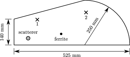
and a height of 5 mm. The excitation frequency $f$ ranges from 1 to 25 GHz. In that range, only one vertical mode of the electric field strength is excited. The Helmholtz equation for the tilted stadium is then mathematically equivalent to the Schrödinger equation of a two-dimensional chaotic quantum billiard Stoeckmann1990 . An Agilent PNA-L N5230A vector network analyzer (VNA) coupled rf energy via one of two antennas labeled $1$ and $2$ into the resonator and determined magnitude and phase of the transmitted (reflected) signal at the other (same) antenna in relation to the input signal and, thus, the elements $S_{ab}(f)$ with $a,b=1,2$ of the complex-valued $2\times 2$ scattering matrix $S(f)$. Distorting effects of the connecting coaxial cables were removed by calibration. We measured the elements of $S(f)$ in the frequency range 1–25 GHz at a resolution of 100 kHz. To improve the statistical significance of the data set, an additional scatterer (an iron disc of 20 mm diameter) was placed within the cavity. It could be freely moved and allowed the measurement of statistically independent spectra, so-called “realizations”.

Time-reversal invariance is violated Schaefer2007 by a ferrite cylinder ($4\pi\,M_{\rm S}=1859~{}{\rm Oe}$, $\Delta H=17.5~{}{\rm Oe}$, courtesy of AFT Materials GmbH, Backnang, Germany) of 4 mm diameter and 5 mm height. The cylinder was placed inside the resonator and magnetized by an external magnetic field $B$. The field was provided by two NdFeB magnets (cylindrical shape, 20 mm diameter and 10 mm height) attached from the outside to the billiard. Field strengths of up to 360 mT could be attained. Here we focus on the results at $B=190~{}{\rm mT}$ as there the effects are most clearly visible. The spins within the ferrite precess collectively with their Larmor frequency about the external field. The rf magnetic fields of the resonator modes are, in general, elliptically polarized and couple to the spins of the ferrite. The coupling depends on the rotational direction of the rf field. An interchange of input and output channels changes the rotational direction and thus the coupling of the resonator modes to the ferrite. Figure 2 demonstrates that reciprocity, defined by $S_{12}(f)=S_{21}(f)$ and implied by ${\mathcal{T}}\,$invariance, is violated.

Figure 2: Transmission spectra for $B=190~{}{\rm mT}$ in the range 16–17 GHz. The amplitudes and phases of $S_{12}$ (solid) and $S_{21}$ (dashed) are seen to differ.

As a measure of the strength of ${\mathcal{T}}$-invariance violation, we define the cross-correlation coefficient $C_{\rm cross}(\epsilon=0)$ where

$$C_{\rm cross}(\epsilon)=\frac{\mathfrak{Re}\left(\langle S_{12}(f)\,S_{21}^{\ast}(f+\epsilon)\rangle\right)}{\sqrt{\langle|S_{12}(f)|^{2}\rangle\,\langle|S_{21}(f)|^{2}\rangle}}\,.$$ (1)

If ${\mathcal{T}}\,$invariance holds, we have $C_{\rm cross}(0)=1$ while for complete breaking of ${\mathcal{T}}\,$invariance $S_{12}$ and $S_{21}$ are uncorrelated and thus $C_{\rm cross}(0)=0$. The average $\langle\,\cdot\,\rangle$ over the data is taken in frequency windows of width $1~{}$GHz and over 6 realizations, i.e., positions of the additional scatterer. The upper panel of Figure 3 shows $C_{\rm cross}(0)$ for the different frequency windows. The cross-correlation coefficient is seen to depend strongly on $f$ although complete violation of ${\mathcal{T}}\,$invariance is never attained. At 5–7 GHz the Larmor frequency of the ferrite matches the rf frequency, and the ferromagnetic resonance directly results in $C_{\rm cross}(0)\approx 0.8$. Around 15 GHz the effects of ${\mathcal{T}}$-invariance violation are strongest, $C_{\rm cross}(0)\approx 0.5$. A third minimum is observed at about 24 GHz. The connection of the latter two minima to the properties of the ferrite is not clear.

Figure 3: Experimentally determined values of $C_{\rm cross}(0)$ (upper panel) from Eq. (1) and the parameter $\xi$ for ${\mathcal{T}}$-invariance violation deduced from these (lower panel) with the help of Eq. (3). The error bars indicate the r.m.s. variation of $C_{\rm cross}(0)$ over the 6 realizations.

Analysis. We analyze the data with a scattering approach developed in the context of compound-nucleus reactions Mahaux1969 . The scattering matrix for the scattering from antenna $b$ to antenna $a$ with $a,b=1,2$ is written as

$$S_{ab}(f)=\delta_{ab}-2\pi\,i\,\big{(}W^{\dagger}\,(f-H^{\rm eff})^{-1}\,W\big{)}_{ab}\,.$$ (2)

The matrix $W_{\mu a}$ is rectangular and describes the coupling of the $N$ resonant states $\mu$ in the cavity with the antennas $a=1,2$. We assume that ${\mathcal{T}}$-invariance violation is due to the ferrite only. Then $W_{\mu a}$ is real. The resonances in the cavity are modeled by $H^{\rm eff}=H-i\pi\,\tilde{W}\tilde{W}^{\dagger}$. Here $H$ is the Hamiltonian of the closed resonator. The elements of the real matrix $\tilde{W}_{\mu c}$ are equal to those of $W_{\mu c}$ for $c=1,2$. As done successfully before Uzy ; Friedrich2008 , Ohmic absorption of the microwaves in the walls of the cavity and the ferrite is mimicked Brouwer1997 by additional fictitious weakly coupled channels $c$. The classical dynamics of a point particle within the tilted stadium billiard is chaotic. Therefore Bohigas1984 , we model $H$ by an ensemble of random matrices. The $N$-dimensional Hamiltonian matrix $H$ of the system (the cavity) is written as the sum of two parts Pandey1981 ; Pandey1983 ; Altland1993 , $H=H^{s}+i(\pi\xi/\sqrt{N})H^{a}$. The real, symmetric, and ${\mathcal{T}}$-invariant matrix $H^{s}$ is taken from the Gaussian Orthogonal Ensemble (GOE) while the real, antisymmetric matrix $H^{a}$ with Gaussian-distributed matrix elements models the ${\mathcal{T}}$-invariance breaking part of $H$. For $\pi\xi/\sqrt{N}=1$ the Hamiltonian $H$ belongs to the Gaussian Unitary Ensemble (GUE) describing systems with complete ${\mathcal{T}}\,$breaking. However, for $N\to\infty$, ${\mathcal{T}}\,$invariance is significantly broken already when the dimensionless parameter $\xi$ is close to unity footnote . In the same limit $C_{\rm cross}(0)$ in Eq. (1) can be expressed analytically in terms of a threefold integral involving the parameter $\xi$. For the derivation we extended the method of Ref. Pluhar1995 where the ensemble average of $|S_{ab}|^{2}$ was computed as function of the parameter $\xi$. The cross-correlation coefficient $C_{\rm cross}(0)$ is obtained by setting $\epsilon=0$, $\sigma=-1$, and $a,b=1,2$ in the function

$$F^{\sigma}_{ab}(\epsilon|T_{a},T_{b},\tau_{\rm abs},\xi)=\frac{1}{8}\int_{0}^{\infty}{\rm d}x_{1}\int_{0}^{\infty}{\rm d}x_{2}\,\int_{0}^{1}{\rm d}x\,$$ (3)

$$\times \frac{\mu(x,x_{1},x_{2})}{\mathcal{F}}\cdot\exp\left(-\frac{i\pi\epsilon}{d}(x_{1}+x_{2}+2x)\right)$$

$$\times \prod_{c}\frac{1-T_{c}\,x}{\sqrt{(1+T_{c}x_{1})(1+T_{c}\,x_{2})}}\Big{[}\Big{\{}J_{ab}(x,x_{1},x_{2})$$

$$\times \left[\mathcal{F}\mathcal{E}_{+}+(\lambda_{2}^{2}-\lambda_{1}^{2})\mathcal{E}_{-}+4\mathfrak{t}\mathcal{R}(\lambda_{2}^{2}\mathcal{E}_{-}+\mathcal{F}(\mathcal{E}_{+}-1))\right]$$

$$+ \sigma\cdot 2(1-\delta_{ab})T_{a}T_{b}\big{[}\mathcal{E}_{-}K_{ab}(\lambda,\lambda_{1},\lambda_{2}|T_{a},T_{b},\xi)$$

$$+ \left(\mathcal{E}_{+}-\frac{\mathcal{E}_{-}}{t\mathcal{F}}\right)L_{ab}(\lambda,\lambda_{1},\lambda_{2}|T_{a},T_{b},\xi)\big{]}\Big{\}}\cdot\exp\left(-2\mathfrak{t}\mathcal{G}_{-}\right)$$

$$+ \left(\lambda_{1}\leftrightarrow\lambda_{2}\right)\Big{]},$$

with the notations

$$\mathfrak{t} = \pi^{2}\,\xi^{2},\quad\mathcal{R}=4(x+x_{1})(x+x_{2}),$$

$$\mathcal{U} = 2\sqrt{x_{1}(1+x_{1})x_{2}(1+x_{2})},\quad\mathcal{F}=4x(1-x),$$

$$\mathcal{E}_{\pm} = 1\pm\exp(-2\mathfrak{t}\mathcal{F}),\quad\lambda=1-2x,$$

$$\lambda_{i} = \sqrt{(1+x_{1})\,(1+x_{2})+x_{1}x_{2}-(-1)^{i}\,\mathcal{U}},$$

$$\mathcal{G}_{i} = \lambda_{i}^{2}-1,i=1,2\,.$$ (4)

The integration measure $\mu(x,x_{1},x_{2})$ and the function $J_{ab}(x,x_{1},x_{2})$ are given explicitly in Ref. Ver85 , while the functions $K_{ab}(\lambda,\lambda_{1},\lambda_{2}|T_{a},T_{b},\xi)$ and $L_{ab}(\lambda,\lambda_{1},\lambda_{2}|T_{a},T_{b},\xi)$ can be read off Eq. (2) of Ref. Gerland . We checked our analytic results by numerical RMT simulations. The parameters of Eq. (3) for $\epsilon=0$ are $\xi$, the transmission coefficients $T_{a}=1-|\langle S_{aa}\rangle|^{2}$ for $a=1,2$, and the sum $\tau_{\rm abs}$ of 300 transmission coefficients that model the Ohmic losses Brouwer1997 ; Friedrich2008 .

For a typical set $T_{1},T_{2},\tau_{\rm abs}$, Fig. 4 shows $C_{\rm cross}(0)$ versus $\xi$. Within the frequency range 1–25 GHz, $C_{\rm cross}(0)$ depends very weakly on $T_{1},T_{2},\tau_{\rm abs}$, and Fig. 4 can be taken to be universal.

Figure 4: Dependence of the cross-correlation coefficient $C_{\rm cross}(0)$ on the parameter $\xi$ as predicted by the random-matrix model for partial violation of ${\mathcal{T}}\,$invariance. Also shown is how $C_{\rm cross}(0)=0.49(3)$ translates into $\xi=0.29(2)$.

For each data point shown in the upper panel of Fig. 3 the corresponding value of $\xi$ was read off Fig. 4 and the result is shown as function of $f$ in the lower panel of Fig. 3. Figure 3 shows that in the interval from 1 to 25 GHz, the ratio of the average resonance width $\Gamma$ to the average resonance spacing $d$ varies from $\Gamma/d\approx 0.01$ to $\Gamma/d\approx 1.2$ while the strength $\xi$ of ${\mathcal{T}}\,$breaking varies from zero to $0.3$. Numerical calculations show that for $\xi=0.3$ the spectral fluctuations of the Hamiltonian $H$ for the closed resonator defined below Eq. (2) almost coincide with those of the GUE Bohigas1995 . We also found that for $\xi=0.4$ they do not differ significantly from those presented in Ref. So1995 , where the conclusion was drawn, that complete ${\mathcal{T}}\,$breaking is achieved. However, even for $\xi=0.4$ the value of $C_{\rm cross}(0)$ is still far from zero. This shows that $C_{\rm cross}(0)$ is a particularly suitable measure of the strength $\xi$ of ${\mathcal{T}}\,$violation.

Autocorrelation function. Since $C_{\rm cross}(0)$ depends only weakly on the values of $T_{1},T_{2}$ and $\tau_{\rm abs}$, we used the autocorrelation function $C_{ab}(\epsilon)$ for a more precise determination of these parameters, especially of $\tau_{\rm abs}$. The function

$$C_{ab}(\epsilon)=\langle S_{ab}(f)\,S_{ab}^{\ast}(f+\epsilon)\rangle-|\langle S_{ab}(f)\rangle|^{2}$$ (5)

was calculated analytically with the method of Ref. Pluhar1995 as a function of $T_{1},T_{2},\tau_{\rm abs},\xi$, and $d$ and is obtained from Eq. (3) by setting $\sigma=+1$. It interpolates between the well-known results for orthogonal symmetry Ver85 (full ${\mathcal{T}}\,$invariance) and for unitary symmetry Fyodorov2005 (complete violation of ${\mathcal{T}}\,$invariance). The mean level spacing $d$ was computed from the Weyl formula. The Fourier transform of the function $C_{ab}(\epsilon)$ was then fitted to the data as in Ref. Friedrich2008 . As starting points we used the values of $T_{1}$ and $T_{2}$ obtained from the measured values of $S_{aa}(f)$ and of $\xi$ determined from $C_{\rm cross}(0)$. For each of the $6$ realizations the spectra of $S_{ab}(f)$ were divided into intervals $\Delta f$ of 1 GHz length. In each interval the Fourier transform $\tilde{C}_{ab}(t_{k})$ of the autocorrelation function (5) was calculated for values of $t_{k}$ between $5~{}{\rm ns}$ and $200~{}{\rm ns}$. The lower limit is determined by the length of the shortest periodic orbit in the classical billiard; for smaller values of $t_{k}$ the Fourier coefficients are nongeneric Bluemel1990 . At $t_{k}\approx 200~{}{\rm ns}$ the values of $\tilde{C}_{ab}(t_{k})$ have decayed over more than three orders of magnitude, and noise limits the analysis. The time resolution was $1/\Delta f=1~{}{\rm ns}$. We measured four excitation functions $S_{ab}(f)$ taking $(a,b)=(1,1),(1,2),(2,1),(2,2$ yielding a total of $4800$ Fourier coefficients for each interval. For $f>$ 10 GHz the fitted values for $T_{1}$ and $T_{2}$ differ by not more than 7 % from the initial ones. (For smaller $f$ the intervals of 1 GHz width comprise only few resonances). The spread of the data is large, see the left panel of Fig. 5. Going to the time domain is useful since the $S_{ab}(f)$ are correlated for neighboring $f$ whereas the correlations are removed in the ratios of the experimental and the fitted values for $\tilde{C}_{ab}(t_{k})$. The latter are stationary and fluctuate about unity. Thus the statistical analysis is much simplified.

Figure 5: Autocorrelation function for $S_{12}$ in the range of 16–17 GHz and at $B=190~{}{\rm mT}$. In the time domain (a) the data (dots) scatter around the theoretical fit (solid) for $T_{1}=0.37$, $T_{2}=0.41$, $\tau_{\rm abs}=2.9$ and $\xi=0.25$. Transforming the results back into frequency domain (b) confirms the good agreement between data and theory. We observe that neighboring data points in (b) are correlated, whereas those in (a) are not.

For each realization the parameters $\tau_{\rm abs}$ and $\xi$ were obtained by fitting the analytical expression for $\tilde{C}_{ab}(t_{k})$ to the experimental results. The values of $\xi$ determined from these fits agree with the ones found from the cross-correlation coefficient. To reduce the spread we combined the data from all realizations within a fixed frequency interval. The result was analyzed with the help of a goodness-of-fit (GOF) test (see Ref. Friedrich2008 ) that distinguishes between full, partial, and no violation of ${\mathcal{T}}\,$invariance. We defined a confidence limit such that the GOF test erroneously rejects a valid theoretical description of the data with a probability of 10 %. With this confidence limit the test rejects the fitted expressions for $\tilde{C}_{ab}(t_{k})$ in only 1 out of the 24 available frequency windows or in 4.2 % of the tests. Thus, the RMT model correctly describes the fluctuations of the $S$-matrix for partial violation of ${\mathcal{T}}\,$invariance in the regimes of isolated and weakly overlapping resonances.

Elastic enhancement factor. As a second test of the theory we use the values of $\xi$ obtained from the cross-correlation coefficients (see Fig. 3) and the parameters $T_{a},T_{b},\tau_{\rm abs}$ resulting from the fit of $\tilde{C}_{ab}(t_{k})$ to predict the values of the elastic enhancement factor $\mathcal{W}=\bigg{(}\langle|S^{\rm fl}_{11}|^{2}\rangle\ \langle|S^{\rm fl}_{22}|^{2}\rangle\bigg{)}^{1/2}/\ \langle|S^{\rm fl}_{12}|^{2}\rangle$ with $S^{\rm fl}_{\rm ab}=S_{\rm ab}-\langle S_{\rm ab}\rangle$ as a function of $f$. We use that $\mathcal{W}=\sqrt{C_{11}(0)\,C_{22}(0)}/C_{12}(0)$, see Eq. (5). For ${\mathcal{T}}$-invariant systems, the elastic enhancement factor decreases from $\mathcal{W}=3$ for isolated resonances with many weakly coupled open channels to $\mathcal{W}=2$ for strongly overlapping resonances ($\Gamma\gg d$). The corresponding values for complete violation of ${\mathcal{T}}\,$invariance are $\mathcal{W}=2$ and $\mathcal{W}=1$, respectively Savin2006 . Figure 6 compares the analytic results for the enhancement factor $\mathcal{W}$ (filled circles) to the data (open circles). For small $f$ (where $\Gamma/d\ll 1$ and $\xi\approx 0$) the experimental results differ from the prediction $\mathcal{W}=3$. Here only few resonances contribute and the errors of the experimental values for $\mathcal{W}$ are large. Moreover $\mathcal{W}$ is determined from only a single value $C_{ab}(0)$ of the measured autocorrelation function while the analytic result is based on a fit of the complete autocorrelation function. As $f$ increases so does $\Gamma/d$, and $\mathcal{W}$ takes values well below 3. At frequencies where $\xi$ is largest $\mathcal{W}$ drops below the value $2$ as predicted, a situation that cannot arise for ${\mathcal{T}}$-invariant systems. The overall agreement between both data sets above $\approx 10~{}{\rm GHz}$ corroborates the confidence in the values of $\xi$ deduced from the cross-correlation coefficients.

Figure 6: Comparison of elastic enhancement factors. For the evaluation of $\mathcal{W}$ the autocorrelation coefficients $C_{ab}(0)$ were determined either directly from the data (open circles) or from the analytic result for partial violation of ${\mathcal{T}}\,$invariance (filled circles) with $\xi$ determined from the cross-correlation coefficient. The error bars indicate the variations within the 6 realizations. The dashed horizontal lines indicate the limits of $\mathcal{W}$ for ${\mathcal{T}}$-invariant systems in the regime of isolated ($\mathcal{W}=3$) or overlapping ($\mathcal{W}=2$) resonances.

Summary. We have investigated partial violation of ${\mathcal{T}}\,$invariance with the help of a magnetized ferrite placed inside a flat microwave resonator (a chaotic billiard) with two antennas. We measured reflection and transmission amplitudes in the regime of isolated and weakly overlapping resonances in the frequency range from $1$ to $25$ GHz and determined the cross-correlation function, the autocorrelation functions, and the elastic enhancement factor from the data. The results were used as a test of random-matrix theory for scattering processes with partial ${\mathcal{T}}\,$violation. That theory yields analytic expressions for all three observables. The parameters of the theory ($T_{1},T_{2},\tau_{\rm abs}$ and the parameter $\xi$ for ${\mathcal{T}}\,$violation) were partly obtained directly from the data but improved values resulted from fits to the autocorrelation function. We find that $0\leq\xi\leq 0.3$. The validity of the theory was tested in two ways. (i) A goodness-of-fit test of the Fourier coefficients of the scattering matrix in frequency intervals of $1$ GHz width yielded excellent agreement. (ii) The elastic enhancement factor predicted from the fitted values of the parameters shows overall agreement with the data for frequencies above $10$ GHz where the experimental errors are small. We conclude that the random-matrix description of $S$-matrix fluctuations with partially broken ${\mathcal{T}}\,$invariance is in excellent agreement with the data.