Permanent address: ]Centro Atómico Bariloche and Instituto Balseiro, 8400 S. C. de Bariloche, Río Negro, Argentina

Lower Bounds on the Exchange-Correlation Energy in Reduced Dimensions

Abstract

Bounds on the exchange-correlation energy of many-electron systems are derived and tested. By using universal scaling properties of the electron-electron interaction, we obtain the exponent of the bounds in three, two, one, and quasi-one dimensions. From the properties of the electron gas in the dilute regime, the tightest estimate to date is given for the numerical prefactor of the bound, which is crucial in practical applications. Numerical tests on various low-dimensional systems are in line with the bounds obtained, and give evidence of an interesting dimensional crossover between two and one dimensions.

In 1979 Lieb lieb79 planted a landmark in quantum many-body physics by proving the existence of a lower bound on the indirect part of the Coulomb interaction. The existence of such a bound is of immediate relevance to such fundamental questions as the stability of matter spruch91 . For the purpose of quantitative calculations, on the other hand, existence of a bound is not enough – one would wish it to be as tight as possible. A tighter version of Lieb’s bound was later derived by Lieb and Oxford lieboxford81 , and it is this tighter form, known as Lieb-Oxford (LO) bound, which is used as key constraint in the construction of many modern density functionals pbe96 ; tpss04 , which in turn are used in calculations of the electronic structure of atoms, molecules, nanoscale systems, and solids.

In connection with recent advances in low-dimensional physics it is important to ask whether LO-like bounds exist and can be formulated also in reduced dimensions, in particular since the study of low-dimensional systems today forms a significant part of condensed-matter and materials physics.

The LO bound lieboxford81 , in its original form, applies to all three-dimensional (3D) nonrelativistic, Coulomb-interacting systems. The bound can be expressed in terms of the indirect part of the interaction energy lieb79 ; lieboxford81 ; levyperdew93 ,

$$W_{xc}[\Psi]\equiv\left<\Psi|{\hat{V}}_{ee}|\Psi\right>-U[n]\geq-\;C_{3}\int d^{3}r\,n^{4/3}({\bf r}),$$ (1)

where the electron-electron (e-e) interaction operator is Coulombic, i.e., ${\hat{V}}_{ee}=\sum_{i>j}|{\bf r}_{i}-{\bf r}_{j}|^{-1}$. Its expectation value is calculated over any normalized many-body wavefunction $\Psi(\mathbf{r}_{1},...,\mathbf{r}_{N})$. $n(\mathbf{r})$ is the corresponding density, and $U[n]$ is the classical Hartree energy. For the prefactor $C_{3}$, where the subscript denotes the number of dimensions $D$, Lieb originally found $C_{3}^{\rm L}=8.52$, which was subsequently refined by Lieb and Oxford to $C^{\rm LO}_{3}=1.68$, and later, numerically, by Chan and Handy to $C^{\rm CH}_{3}=1.64$  chanhandy99 . Recent numerical studies odashimacapelle07 ; odashimacapelle08 , as well as modeling of the prefactor based on its known properties odashimatrickeycapelle08 , have given evidence that the bound can be further tightened.

In two-dimensions (2D), Lieb, Solojev and Yngvason liebsolovejyngvason (LSY) showed that

$$W_{xc}[\Psi]\geq-\;C_{\rm 2}\int d^{2}r\,n^{3/2}({\bf r}),$$ (2)

where $C^{\rm LSY}_{2}=192\sqrt{2\pi}\approx 481\gg C_{3}^{\text{LO}}$. For a $D$-dimensional system, the bound may be written as

$$W_{xc}[\Psi]\geq-\;C_{D}\int d^{D}r\,n^{\alpha}({\bf r}),$$ (3)

but we note that the existence of a bound of this form has been rigorously proven for only 3D and 2D, and that the tightest possible form (i.e., the smallest possible value of $C_{D}$) is unknown in all dimensions.

In this paper we (i) show that the exponents of $n$ in Eqs. (1) and (2) are consequences of universal scaling properties of the e-e interaction; (ii) use this result to deduce the exponent $\alpha$ of a possible one-dimensional (1D) bound; (iii) provide an estimate of the prefactor $C_{D}$ that corresponds to a dramatic tightening of $C^{\rm LSY}_{2}$, smaller but still significant tightening of $C^{\rm LO}_{3}$, and the first proposal for $C_{1}$; (iv) observe unexpected parameter independence and generality of the bound with respect to the model chosen for interactions in 1D; and (v) test the 1D and 2D bounds against analytical and near-exact numerical data for various low-dimensional systems.

The 1D case, in fact, is subtle because the Coulomb interaction is ill-defined. Hence, we consider a contact interaction, ${\hat{V}}_{ee}=\eta\sum_{i>j}\delta(x_{i}-x_{j})$ with $\eta>0$. The discussion below on the 1D case refers to this type of interaction. However, we consider also a soft-Coulomb interaction, ${\hat{V}}_{ee}=\sum_{i>j}\left[(x_{i}-x_{j})^{2}+a^{2}\right]$, which corresponds to a quasi-1D (q1D) situation.

Under homogeneous scaling of the coordinates, ${\bf r}\rightarrow\gamma{\bf r}$ ($0<\gamma<\infty$) levyperdew93 , the $(DN)$-dimensional many-body wavefunction scales as $\Psi({\bf r}_{1}\ldots{\bf r}_{N})\rightarrow\Psi_{\gamma}({\bf r}_{1}\ldots{\bf r}_{N})=\gamma^{DN/2}\Psi(\gamma{\bf r}_{1}\ldots\gamma{\bf r}_{N})$, preserving normalization. This yields the number-conserving scaled density $n({\bf r})\rightarrow n_{\gamma}({\bf r})=\gamma^{D}n(\gamma{\bf r})$. On the other hand, $W_{xc}[\Psi]\rightarrow W_{xc}[\Psi_{\gamma}]=\gamma W_{xc}[\Psi]$, since both the Coulomb ($D=2,3$) and contact ($D=1$) interaction, and their Hartree approximations scale linearly. Thus, Eq. (3) becomes

$$\gamma W_{xc}[\Psi]\geq-\;C_{D}\;\gamma^{D(\alpha-1)}\int d^{D}r\,n^{\alpha}({\bf r}),$$ (4)

and consistency between Eqs. (3) and (4) immediately yields $\gamma=\gamma^{D(\alpha-1)}$, giving $\alpha=1/D+1$. For $D=3$ and $D=2$ this yields $\alpha=4/3$ and $\alpha=3/2$, respectively, in agreement with the LO and LSY bounds. We thus find that if a bound of this form exists, its exponent is, in all dimensions, uniquely determined by coordinate scaling, without requiring the complicated analysis performed in Refs. lieb79 , lieboxford81 , and liebsolovejyngvason . For a LO-like bound in 1D, the same scaling argument suggests the form $W_{xc}[\Psi]\geq-\;C_{1}\int d^{1}r\,n^{2}({\bf r})$, although the existence of such a bound in 1D is at present only a conjecture.

The exponent $\alpha=1/D+1$ in Eq. (4) is the same as in the expression of the exchange energy, $E_{x}[n]$, of the homogeneous $D$-dimensional electron gas, which is applied in the local-density approximation (LDA) GV to the inhomogeneous case. Thus, we can express the right-hand side of all LO-like bounds in terms of

$$E_{x}^{\rm LDA}[n]=-\;A_{D}\int d^{D}r\,n^{\alpha}({\bf r}),$$ (5)

where $A_{3}=3^{4/3}\pi^{-1/3}/4$, $A_{2}=2^{5/2}\pi^{-1/2}/3$, and $A_{1}=\eta/4$  GV . For ground-state densities, the left-hand-side of Eq. (3) can be written in terms of the full exchange-correlation energy, $E_{xc}[n]\equiv W_{xc}[n]+T_{c}[n]\geq W_{xc}[n]$, where the inequality follows from the positiveness of the kinetic-energy part $T_{c}$ of the correlation energy, and the density functional $W_{xc}[n]$ is obtained by evaluating $W_{xc}[\Psi]$ with the wavefunction minimizing $\left\langle\Psi\left|\widehat{T}+\widehat{V}_{ee}\right|\Psi\right\rangle$ under the constraint of reproducing the ground-state density $n(\mathbf{r})$. We can now cast the bound in the form

$$E_{xc}[n]\geq\lambda_{D}\;E_{x}^{\rm LDA}[n],$$ (6)

where $\lambda_{D}=C_{D}/A_{D}$. Thus, the tightest possible bound can be obtained by looking for the maximum value of the density functional

$$\lambda_{D}[n]=\frac{E_{xc}[n]}{E_{x}^{\rm LDA}[n]}=\frac{E_{x}[n]}{E_{x}^{\rm LDA}[n]}+\frac{E_{c}[n]}{E_{x}^{\rm LDA}[n]}$$ (7)

over all possible $D$-dimensional many-body systems. Clearly, this maximization cannot be performed in practice. However, we can make an educated guess as to what the resulting maximum will be.

First, we note that for 3D, it was shown rigorously that the constant $\lambda_{3}$ in Eq. (6) can be replaced by a monotonic function depending on particle number, $\lambda_{3}(N)$, which assigns to all systems with particle number $N$ a common value $\lambda_{3}(N)\leq\lambda_{3}(N\to\infty)\equiv\lambda_{3}$, such that a LO-like bound with $\lambda(N)$ in place of $\lambda$ holds for all systems with this $N$ lieboxford81 ; odashimatrickeycapelle08 . The values commonly quoted for $\lambda_{3}^{\rm L}$, $\lambda_{3}^{\rm LO}$, and $\lambda_{3}^{\rm CH}$ are actually estimates of $\lambda_{3}(N\to\infty)$. To obtain the tightest possible universal ($N$-independent) bound we thus take $N\to\infty$.

Second, we may expect that $E_{x}$ is always relatively close to $E_{x}^{\rm LDA}$, as the particle density $n$ is varied over different physical systems. Hence, the functional $\lambda_{D}[n]$ is expected to be largest for systems where the rightmost ratio in Eq. (7) is largest, i.e., where correlation is largest relative to exchange. This situation is typical of the extreme low-density limit $n\to 0$.

Taken together, the rigorous property of a maximum at $N\to\infty$, and the nonrigorous but reasonable requirement that $n\to 0$, suggest that the largest possible value of $\lambda_{3}[n]$ is obtained for the $r^{\rm 3D}_{s}\rightarrow\infty$ limit of the 3D electron gas (3DEG) with the density parameter $r^{\rm 3D}_{s}=3^{1/3}(4\pi n)^{-1/3}$ perdewwang . This expectation leads to $\lambda_{3}\equiv\lambda_{\rm 3DEG}[r^{\rm 3D}_{s}\rightarrow\infty]=1+\epsilon_{c}(r^{\rm 3D}_{s}\rightarrow\infty)/\epsilon_{x}(r^{\rm 3D}_{s}\rightarrow\infty)=1.9555$ odashimacapelle07 , where $\epsilon_{x}$ ($\epsilon_{c}$) is the exchange (correlation) energy per electron. We note that the original LO bound with $C_{3}^{\rm LO}=1.68$ corresponds to $\lambda_{3}^{\rm LO}=2.27$, while the present estimate $\lambda_{3}=1.9555$ is tighter, and consistent with the empirical prefactor obtained by evaluating $\lambda_{3}[n]$ for real systems  odashimacapelle07 .

We now assume that the above argument about the maximum of $\lambda_{3}$ carries over to reduced dimensions. For the 2D electron gas (2DEG) with $r_{s}^{\rm 2D}=1/\sqrt{\pi n}$ we have $\epsilon_{x}(r_{s}^{\rm 2D})=-4\sqrt{2}/(3\pi r^{\rm 2D}_{s})$. From the Madelung energy of the Wigner crystal bonsall we extract that the leading contribution to the correlation in the low-density limit is $\epsilon_{c}(r_{s}^{\rm 2D}\rightarrow\infty)=-0.509/r_{s}^{\rm 2D}+0.815/\left(r_{s}^{\rm 2D}\right)^{3/2}$. Thus we find $\lambda_{2}\equiv\lambda_{\rm 2DEG}[r^{\rm 2D}_{s}\rightarrow\infty]=1.84$, which is a dramatic improvement on the rigorous mathematical result of Ref. liebsolovejyngvason that $\lambda_{2}\leq\lambda_{2}^{\rm LSY}\approx 452$.

Analogously, for the 1D electron gas (1DEG) with a contact interaction and $r_{s}^{\rm 1D}=1/2n$ we find $\epsilon_{x}(r_{s}^{\rm 1D})=-\eta/(8r^{\rm 1D}_{s})$. The leading contribution to the correlation energy in the low-density limit is $\epsilon_{c}(r_{s}^{\rm 1D}\rightarrow\infty)=-\eta/(8r_{s}^{\rm 1D})+\pi^{2}/32(r_{s}^{\rm 1D})^{2}$ magyarburke04 , yielding $\lambda_{1}\equiv\lambda_{\rm 1DEG}[r^{\rm 1D}_{s}\rightarrow\infty]=2$. Note that this is a general result, in the sense that it does not depend on the parameter $\eta$ of the contact interaction.

Finally, in the q1D system with a soft-Coulomb interaction we first note that the scaling of $W_{xc}$ is nontrivial due additional scaling of the parameter $a$: $W_{xc}^{a}[\Psi]\rightarrow W_{xc}^{a}[\Psi_{\gamma}]=\gamma W_{xc}^{\gamma a}[\Psi]$. Second, for the LDA in Eq. (5) we have now $A_{\text{q1D}}=1/2$, $\alpha=2$, and in the limit $a\rightarrow 0$ the integrand is multiplied by a function $f^{a}[n(x)]=\ln[2/\pi an(x)]+3/2-\mu$, where $\mu\simeq 0.577$ is Euler’s constant fogler . Note the scaling property $f^{a}[n(x)]\rightarrow f^{a}[n_{\gamma}(x)]=\gamma f^{\gamma a}[n(x)]$. Now, we assume that the LO bound in q1D also has this form, i.e., the integrand of the q1D expression for $W_{xc}$ [Eq. (3)] is multiplied by the same factor $f^{a}[n(x)]$. Under this assumption, we may search for the maximum values for $\lambda_{\rm q1D}[n]$ in Eq. (7) in a similar fashion as in 3D, 2D, and 1D.

In the low-density limit of the q1D electron gas (q1DEG) we have $\epsilon_{x}(r_{s}^{\rm q1D}\rightarrow\infty)=n[\ln(a\pi n/2)-3/2+\mu]/2$ and $\epsilon_{c}(r_{s}^{\rm q1D}\rightarrow\infty)=n[\ln(an/2\pi)+3/2+\mu]/2$ fogler . Hence, we find $\lambda_{\rm q1D}\equiv\lambda_{\rm q1DEG}[r^{\rm q1D}_{s}\rightarrow\infty]=2$. We note, again, that the leading contribution to $\lambda_{\rm q1DEG}$ is independent of the softening parameter $a$ of the q1D model.

Moreover, we note the highly nontrivial fact that the leading contribution to $\lambda_{\rm 1DEG}$ and $\lambda_{\rm q1DEG}$ is the same. This encourages us to propose $\lambda_{D}=2$ as the tightest general bound for both 1D and q1D. It is also important to note that in 2D, 1D, and q1D, the correction to the leading term is negative, decreasing the value of the corresponding $\lambda_{D}$ for finite (non-vanishing) densities, in line with our proposal to extract the maximum of $\lambda_{D}[n]$ from the low-density limit of the electron gas. The results for the tightest bounds in different dimensions are summarized in Table 1.

Table 1: Estimated prefactors $\lambda_{D}=C_{D}/A_{D}$ for bounds on $E_{xc}$ and $W_{xc}$, compared to literature values, in different dimensions. The quasi-one-dimensional (q1) case involves special conditions (see text).

$D$	3	2	1	q1
$\lambda_{D}^{\rm here}$	1.96	1.84	2.0	2.0
$\lambda_{D}^{\rm lit}$	2.27 lieboxford81	452 liebsolovejyngvason	-	-

Next, we test our bounds against analytical and near-exact numerical data obtained independently for low-dimensional systems, in a similar spirit as was done for 3D systems in Ref. odashimacapelle07 . In particular, we consider 2D parabolic (harmonically confined) and hard-wall square quantum dots qd-reviews (QDs), where the density parameter can be estimated as $r_{s}=N^{-1/6}\omega^{-2/3}$ (Ref. koskinen ) and $r_{s}=(\pi N)^{-1/2}L$ (Ref. polygonal ), respectively (2D indication omitted for clarity). Here $\omega$ is the harmonic confinement strength, $L$ is the side length of the square QD, and $N$ is the number of electrons.

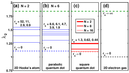
Figure 1: (Color online) Values for $\lambda_{2}[n]$ in different finite and infinite 2D systems compared to our limit $\lambda_{2}=1.84$ (thick dashed line).

Figure 1(a) shows $\lambda_{2}[n]$ for a 2D Hooke’s atom, which is equivalent to a parabolic QD with $N=2$. Here we focus on some of the analytical two-electron solutions in the range $r_{s}=0.9\ldots 52$ derived by Taut taut . The maximum value $\max(\lambda_{2,{\rm Hooke}})\approx 1.55$ is relatively close to the corresponding 3D result $\max(\lambda_{3,{\rm Hooke}})\approx 1.49$ (Ref. odashimacapelle07 ). Detailed analysis of the low-density behavior of $\lambda_{2}$ is given below. In the noninteracting (high-density) limit, where the correlation energy is zero, we find numerically $\lambda_{2,{\rm Hooke}}^{\omega\rightarrow\infty}=E_{x}/E_{x}^{\mathrm{LDA}}\approx 1.10$ which is slightly below the corresponding 3D value odashimacapelle07 of 1.17.

In larger QD systems ($N>2$), most reference data are given only in terms of ground-state total energies $E_{\mathrm{tot}}$, whereas the calculation of $\lambda_{D}[n]$ requires knowledge of the exact exchange-correlation energy and the electron density $n$. The exact DFT correlation energy can be computed as $E_{c}[n^{\mathrm{exact}}]=E_{\mathrm{tot}}[n^{\mathrm{exact}}]-E_{\mathrm{tot}}^{\mathrm{EXX}}[n^{\mathrm{exact}}]$ where $E_{\mathrm{tot}}$ is the exact total energy and EXX refers to exact exchange. To estimate $\lambda_{D}[n^{\mathrm{exact}}]$, we may then perform a self-consistent EXX calculation and calculate

$$\lambda_{D}\approx\frac{E_{x}^{\mathrm{EXX}}[n^{\mathrm{EXX}}]+E_{\mathrm{tot}}[n^{\mathrm{exact}}]-E_{\mathrm{tot}}^{\mathrm{EXX}}[n^{\mathrm{EXX}}]}{E_{x}^{{\mathrm{LDA}}}[n^{\mathrm{EXX}}]}.$$ (8)

In this work we have performed the EXX calculations in the Krieger-Li-Iafrate (KLI) approximation KLI within the octopus real-space density-functional code octopus . We note that according to our numerical test for the 2D Hooke’s atom, the estimate in Eq. (8) yields generally larger values for $\lambda_{D}[n]$ than the definition in Eq. (7).

Figure 1(b) shows results for a parabolic QD with $N=6$. Here we use as the reference data the variational quantum Monte Carlo (QMC) total energies in the weak-confinement regime ari_wigner . In Fig. 1(c) we present results for square-well QDs with $L=\pi$ and varying $N$. Again, we use variational QMC data for the total energies recta . Comparison with fixed $r_{s}$ to parabolic – and also to circular-well QDs (not shown) – reveals that deformation from the circular geometry decreases $\lambda_{2}[n]$. Similar decrease in $\lambda_{2}[n]$ is found if the circular confinement is made elliptic in the $r_{s}=0$ limit (not shown).

The $r_{s}=0$ limit allows testing also within circular confinement by varying the curvature, i.e., the exponent in $V_{\mathrm{circular}}(r)=|r|^{\alpha}$. Interestingly, the largest value for $\lambda_{2}$ is obtained at the smallest $\alpha$ we can numerically consider, i.e., at $\alpha=0.5$, which gives $\lambda_{2}[n]=1.110$. Overall, the numerical results summarized in Fig. 1 show that in both finite and infinite 2D systems, values obtained for $\lambda_{2}[n]$ are consistently below our limit $\lambda_{2}=1.84$ (thick dashed line).

Finally we consider the low-density limit of the 2D Hooke’s atom in detail. In Fig. 2

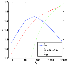
Figure 2: (Color online) Values for $\lambda_{2}[n]$ in a two-dimensional Hooke’s atom as a function of $r_{s}=2^{-1/6}\omega^{-2/3}$. The circles connected by solid lines correspond to $\lambda_{2}[n]$ in the definition of Eq. (7). The dashed line shows the auxiliary quantity $\lambda^{*}[n]$ (see text). The dotted line corresponds to the quasi-one-dimensional result.

we show $\lambda_{2}[n]$ (solid line) up to the extreme low-density regime. As expected, $\lambda_{2}[n]$ first increases as a function of $r_{s}$. However, at $r_{s}\sim 50$, we find an local maximum of $\lambda_{2}[n]\approx 1.55$ [see also Fig. 1(a)] followed by a decrease at higher $r_{s}$. By contrast, if the (2D) LDA exchange in Eq. (7) is replaced by exact exchange, $\lambda_{2}[n]\rightarrow\lambda^{*}[n]:=E_{\mathrm{xc}}/E_{x}=1+E_{c}/E_{x}$, the behavior is monotonic (dashed line) as expected. Note, however, that $\lambda^{*}[n]$ is not the quantity used in the LO bound, but is used here as an auxiliary quantity. Examination of the total electron density in the low-density regime suggests that the unexpected behavior of $\lambda_{2}[n]$ in Fig. 2 is due to the breakdown of the 2D-LDA. Namely, as the confinement is made weaker, the electrons are pushed further apart from each other leading to a q1D ring-shaped total density. In fact, the low-density regime in Fig. 2 shows reasonable agreement between $\lambda^{*}$ and the q1D result (dotted line) deduced from Fogler fogler with the parameter $a$ estimated from the low-density ring-like model by Taut taut . Hence, it is evident that decreasing the density in a 2D Hooke’s atom leads to a dimensional crossover.

To summarize, we have shown that the exponents in Eqs. (1) and (2) are consequences of universal scaling properties of the electron-electron interaction. We have thus been able to deduce the exponent $\alpha$ of a one-dimensional bound. Furthermore, we have provided a tightening of the prefactor of the three-dimensional bound, a dramatic tightening of the prefactor in two-dimensions, and the first proposal for the prefactor in one dimension. Unexpected generality of the bound with respect to the type of interactions in one- and quasi-one-dimensional systems was observed. Our numerical tests for low-dimensional model systems are consistent with the derivations, all showing $\lambda_{2}[n]<\lambda_{2}$, and display an interesting dimensional crossover in the low-density limit. Besides their general relevance in quantum many-body physics, these results provide constraints for accurate approximations of the exchange-correlation functionals in any dimension.

- (1) E. H. Lieb, Phys. Lett. 70A, 444 (1979).
- (2) L. Spruch, Rev. Mod. Phys. 63, 151 (1991).
- (3) E. H. Lieb and S. Oxford, Int. J. Quantum Chem. 19, 427 (1981).
- (4) J. P. Perdew, K. Burke, and M. Ernzerhof, Phys. Rev. Lett. 77, 3865 (1996); erratum Phys. Rev. Lett. 78, 1396 (1997).
- (5) J. P. Perdew et al., J. Chem. Phys. 120, 6898 (2004).
- (6) M. Levy and J. P. Perdew, Phys. Rev. B 48, 11638 (1993).
- (7) G. K.-L. Chan and N. C. Handy, Phys. Rev. A 59, 3075 (1999).
- (8) M. M. Odashima and K. Capelle, J. Chem. Phys. 127, 054106 (2007).
- (9) M. M. Odashima and K. Capelle, Int. J. Quantum Chem. 108, 2428 (2008).
- (10) M. M. Odashima, K. Capelle, and S. B. Trickey, J. Chem. Theory Comput. 5, 798 (2009).
- (11) E. H. Lieb, J. P. Solovej, and J. Yngvason, Phys. Rev. B 51, 10646 (1995).
- (12) G. F. Giuliani and G. Vignale, in Quantum Theory of the Electron Liquid, (Cambridge University Press, Cambridge, 2005).
- (13) J. P. Perdew and Y. Wang, Phys. Rev. B 45, 13244 (1992).
- (14) L. Bonsall and A. A. Maradudin, Phys. Rev. B 15, 1959 (1977).
- (15) R. J. Magyar and K. Burke, Phys. Rev. A 70, 032508 (2004), Phys. Rev. A 72, 029901(E) (2005).
- (16) M. M. Fogler, Phys. Rev. Lett. 94, 056405 (2005).
- (17) For a review, see, e.g., S. M. Reimann and M. Manninen, Rev. Mod. Phys. 74 1283 (2002).
- (18) M. Koskinen, M. Manninen, and S. M. Reimann, Phys. Rev. Lett. 79, 1389 (1997).
- (19) E. Räsänen, et al., Phys. Rev. B 67, 035326 (2003).
- (20) M. Taut, J. Phys. A 27, 1045 (1994).
- (21) J. B. Krieger, Y. Li, and G. J. Iafrate, Phys. Rev. A 46, 5453 (1992).
- (22) M. A. L. Marques et al., Comp. Phys. Comm. 151, 60 (2003); A. Castro et al., Phys. Stat. Sol. (b) 243, 2465 (2006).
- (23) A. Harju, S. Siljamäki, and R. M. Nieminen, Phys. Rev. B 65, 075309 (2002).
- (24) E. Räsänen et al., Phys. Rev. B 67, 235307 (2003).