Efficient quantum algorithm for preparing molecular-system-like states on a quantum computer

Abstract

We present an efficient quantum algorithm for preparing a pure state on a quantum computer, where the quantum state corresponds to that of a molecular system with a given number $m$ of electrons occupying a given number $n$ of spin orbitals. Each spin orbital is mapped to a qubit: the states $|1\rangle$ and $|0\rangle$ of the qubit represent, respectively, whether the spin orbital is occupied by an electron or not. To prepare a general state in the full Hilbert space of $n$ qubits, which is of dimension $2^{n}$, $O(2^{n})$ controlled-NOT gates are needed, i.e., the number of gates scales exponentially with the number of qubits. We make use of the fact that the state to be prepared lies in a smaller Hilbert space, and we find an algorithm that requires at most $O(2^{m+1}n^{m}/{m!})$ gates, i.e., scales polynomially with the number of qubits $n$, provided $n\gg m$. The algorithm is simulated numerically for the cases of the hydrogen molecule and the water molecule. The numerical simulations show that when additional symmetries of the system are considered, the number of gates to prepare the state can be drastically reduced, in the examples considered in this paper, by several orders of magnitude, from the above estimate.

I introduction

Simulating quantum systems on a classical computer is a hard problem. The size of the Hilbert space of the simulated system increases exponentially with the system size. For example, in quantum chemistry, the full configuration interaction (FCI) method diagonalizes the molecular Hamiltonian to provide solutions to the electronic structure problem. The resource requirement for performing the FCI calculation scales exponentially with the size of the system helgaker . Therefore, it is restricted to the treatment of small diatomic and triatomic systems LJ . Feynman fey observed that simulating a quantum system might be more efficient on a quantum computer than on a classical computer. Further work has born out of this early suggestion lloyd ; zalka ; abrams ; lidarwang ; man ; aa ; whf ; guzikdyn ; nori ; bul ; you .

The implementation of a quantum simulation algorithm requires a mapping from the system wave function to the state of the qubits. One possible mapping is through the Jordan-Wigner transformation (JWT) JWT . Each spin orbital is mapped to a qubit: the states $|1\rangle$ and $|0\rangle$ of the qubit represent, respectively, whether the spin orbital is occupied by an electron or not. The simulated system, and therefore the quantum computer, can be in a quantum superposition of different configurations. In quantum chemistry, this quantum superposition is known as the configuration state function (CSF). There are other possible mappings between the simulated system and the quantum computer aa ; whf . For example, one can make use of the fact that the Hilbert space of interest, i.e., one with $m$ electrons occupying $n$ spin orbitals, is of dimension $\left(\begin{array}[]{c}n\\ m\end{array}\right)$, and use the smallest number $n^{\prime}$ of qubits that satisfies the condition $2^{n^{\prime}}\geq\left(\begin{array}[]{c}n\\ m\end{array}\right)$. The Hilbert space of the quantum computer would then be large enough to describe any quantum state of the simulated system. However, since these compact mappings complicate the implementation of the simulation, we only consider the simple mapping explained above.

Preparing a general pure state in the full Hilbert space of $n$ qubits, which is of dimension $2^{n}$, has been studied by several groups. Shende and Markov shende and Möttönen et al. mott showed that preparing a generic $n$-qubit pure state from $|0\rangle^{\otimes n}$ requires $O(2^{n})$ controlled-NOT (CNOT) gates, which gives an exponential scaling for the number of CNOT gates; Bergholm et. al. berg gave an upper bound for the number of gates required for transforming an arbitrary state $|a\rangle$ to an arbitrary state $|b\rangle$: ($2^{n+1}-2n-2$) CNOT gates and ($2^{n+1}-n-2$) one-qubit gates. The gate count is halved if $|a\rangle$ or $|b\rangle$ is one of the basis configuration states. Another quantum algorithm for the preparation of an arbitrary pure state with fidelity arbitrarily close to one was suggested by Soklakov and Schack sok , which is based on Grover’s quantum search algorithm.

In this paper, we study the preparation of a pure state in the second-quantized representation that represents the quantum state of $m$ electrons distributed among $n$ spin orbitals. The state to be prepared lies in the combinatorial space of dimension $\left(\begin{array}[]{c}n\\ m\end{array}\right)$, which is a subspace of the full Hilbert space of $n$ qubits. Ortiz et al. ortiz studied a similar problem, and they gave an algorithm for preparing a state that is composed of $N$ configurations, where $N$ is a finite and small number. Their algorithm scales as $O(N^{2}n^{2})$, where $n$ is the number of the qubits. In this paper we present an efficient recursive algorithm that gives specific quantum circuit for preparing a pure state, with polynomial scaling of the number of CNOT gates in terms of the number of the qubits. We have numerically simulated the state preparation algorithm to prepare the electronic states of the hydrogen and the water molecules. The results show that the number of CNOT gates can be reduced by up to $3$ orders of magnitude from the upper bound we derive.

The structure of this work is as follows. In Sec. II we discuss mapping the Fock space of the system onto the Hilbert space of the qubits. In Sec. III we present a recursive algorithm for state preparation. Preparing a general pure state in the one-electron systems is discussed in detail. Then based on the results for the one-electron system, a recursive approach for preparing a general state of an $m$-electron system is presented. In Sec. IV, we discuss the simplification of the two-fold controlled unitary operations in the algorithm. In Sec. V, we analyze the scaling of the algorithm. In Sec. VI, we apply the algorithm to prepare the electronic states of the hydrogen and the water molecules. We close with a conclusion section.

II Fock space of molecular systems and the Jordan-Wigner Transformation

The wave function of a $m$-electron, $n$-spin-orbital system is a linear combination of Slater determinants. In the formalism of second quantization it is written as:

$$|\Psi\rangle=\sum_{\begin{subarray}{c}i_{1},\text{ }\cdots,\text{ }i_{n}\in\{0,1\}\\ i_{1}\text{ }+\text{ }\cdots\text{ }+\text{ }i_{n}=m\end{subarray}}k_{i_{1},\cdots,i_{n}}(a_{1}^{\dagger})^{i_{1}}\cdots(a_{n}^{\dagger})^{i_{n}}|\Omega\rangle,$$ (1)

where $|\Omega\rangle$ represents the vacuum state with no electrons. Each set $\{i_{1},\cdots,i_{n}\}$ represents an electron configuration of the system, and these states are used as the basis vectors of the configuration space of the system. The fermion creation and annihilation operators $a_{j}^{{\dagger}}$ and $a_{j}$ satisfy the canonical anticommutation relations $\{a_{i},a_{j}\}=0;\{a_{i},a_{j}^{{\dagger}}\}=\delta_{ij}$. $a_{j}^{{\dagger}}$ ($a_{j}$) creates (annihilates) a fermion on the $j$th spin orbital.

The fermion algebra is isomorphic to the standard quantum computing (QC) model (or Pauli) algebra. The isomorphism is established through the Jordan-Wigner transformation JWT . The JWT maps a fermion state to a one-dimensional standard QC state and vice versa. The creation and annihilation operators for the fermion state are mapped to the Pauli operators through the JWT,

$$a_{j}\rightarrow[\Pi_{i=1}^{j-1}(-\sigma_{z}^{i})]\sigma_{-}^{j},$$ (2)

$$a_{j}^{{\dagger}}\rightarrow[\Pi_{i=1}^{j-1}(-\sigma_{z}^{i})]\sigma_{+}^{j},$$ (3)

where $\sigma_{z}$ is the Pauli matrix defined as:

$$\sigma_{z}=\left(\begin{array}[]{cc}1&0\\ 0&-1\end{array}\right).$$ (4)

The operators $\sigma_{-}$ and $\sigma_{+}$ are the Pauli lowering and raising operators defined as:

$$\sigma_{-}=\frac{1}{2}(\sigma_{x}-i\sigma_{y})=\left(\begin{array}[]{cc}0&0\\ 1&0\end{array}\right),$$ (5)

$$\sigma_{+}=\frac{1}{2}(\sigma_{x}+i\sigma_{y})=\left(\begin{array}[]{cc}0&1\\ 0&0\end{array}\right).$$ (6)

They satisfy the following conditions:

$$\sigma_{+}|0\rangle=0,\qquad\sigma_{-}|0\rangle=|1\rangle,$$ (7)

and

$$\sigma_{+}|1\rangle=|0\rangle,\text{ \ \ \ \ }\sigma_{-}|1\rangle=0,$$ (8)

where

$$|0\rangle=\left(\begin{array}[]{c}1\\ 0\end{array}\right),\qquad|1\rangle=\left(\begin{array}[]{c}0\\ 1\end{array}\right).$$ (9)

III recursive algorithm for state preparation

State preparation means starting from a standard initial state on a quantum computer and, by applying a unitary operation, transforming it to a given target state. In this paper, the target state in general is an entangled state mapped from a state in the Fock space of the $m$-electron, $n$-spin-orbital system. The unitary operation can be decomposed into a sequence of elementary quantum gates.

Our approach for state preparation is as follows: instead of starting from the initial state and transforming it to the target state, we start from the target state and transform it to the initial state. We can obtain the gate sequence for preparing the target state by inverting the quantum circuit sequence, since any unitary operation is reversible. A recursive procedure is applied in our “reverse engineering$"$ approach. We first solve the problem of state preparation for one-electron system, then based on this, the general state preparation for $m$-electron system is solved.

We set the initial state of an $n$-qubit system to be $|0\rangle^{\otimes n}$ and define the target state as:

$$|\Psi_{T}\rangle=\sum_{i=1}^{N}k_{i}|\psi_{i}\rangle,$$ (10)

where $N$ is the dimension of the configuration space and

$$\sum_{i=1}^{N}|k_{i}|^{2}=1,$$ (11)

where $|\psi_{i}\rangle$ is a single configuration that describes a distribution of $m$ electrons on $n$ spin orbitals. The states $\{|\psi_{i}\rangle\}$ are the basis vectors of the configuration space. For example, the state $\frac{1}{\sqrt{3}}|001\rangle+\frac{1}{\sqrt{6}}|010\rangle+\frac{1}{\sqrt{2}}|100\rangle$ is composed of three configurations in the state space of a one-electron, three-spin-orbital system.

III.1 Gate library

The gate library used in our approach contains the CNOT gate and the single qubit gates $C$. Here $C$ represents all unitary single qubit operators in SU($2$). It can be written in the form:

$$C=u|0\rangle\langle 0|+v|1\rangle\langle 0|-v^{\ast}|0\rangle\langle 1|+u^{\ast}|1\rangle\langle 1|=\left(\begin{array}[]{cc}u&-v^{\ast}\\ v&u^{\ast}\end{array}\right)$$ (12)

where $u$ and $v$ are complex numbers and

$$|u|^{2}+|v|^{2}=1.$$ (13)

The Hadamard gate $H$ and the NOT gate $X$ are included in $C$. We define another class of operators $\widetilde{H}$, which is a sub-class of the single-qubit operator $C$, such that:

$$\widetilde{H}=C^{{\dagger}}XC=\left(\begin{array}[]{cc}u^{\ast}v+uv^{\ast}&{u^{\ast}}^{2}-{v^{\ast}}^{2}\\ u^{2}-v^{2}&-(u^{\ast}v+uv^{\ast})\end{array}\right),$$ (14)

for some $C$. We call $\widetilde{H}$ the generalized Hadamard gate. It has the same property as the Hadamard gate, $\widetilde{H}\widetilde{H}=I$, and acts in a similar way as the Hadamard gate. Just like the Hadamard gate transforms a superposition state $\frac{1}{\sqrt{2}}(|0\rangle+|1\rangle)$ of a single qubit to state $|0\rangle$ and $\frac{1}{\sqrt{2}}(|0\rangle-|1\rangle)$ to state $|1\rangle$, the $\widetilde{H}$ gate transforms a given superposition state $a|0\rangle+b|1\rangle$ of a single qubit to state $|0\rangle$ or $|1\rangle$.

A considerable effort has been made to synthesize two-qubit circuits using CNOT gates and single-qubit gates vidal ; vatan ; vshende ; zhang and quantum logic circuits vart ; mot ; vvvshende ; tuc . It has been shown that to implement a typical two-qubit operator, three CNOT gates are needed. In this paper we only use two kinds of two-qubit gates: the CNOT gate and the controlled-$\widetilde{H}$ gate, $C$-$\widetilde{H}$, which as shown in Fig. $1$, contains only one CNOT gate. In our algorithm, the $\widetilde{H}$ and $C$-$\widetilde{H}$ gates are used to address the configuration coefficients and reduce the number of the configurations that span the target state $|\Psi_{T}\rangle$ until it reaches the initial state $|0\rangle^{\otimes n}$. An example for transforming a three qubit state to the initial state is shown below.

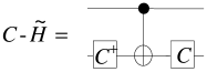
Figure 1: Quantum circuit for the controlled-$\widetilde{H}$ gate.

To transform the target state to the initial state, we first disentangle the target state, then reduce the number of configurations in the target state by applying $\widetilde{H}$ and $C$-$\widetilde{H}$ gates. A simple example for a Bell-type state $|\beta\rangle=a|10\rangle+b|01\rangle$ is shown as follows: to transform this state to the initial state $|00\rangle$, first we apply the $X^{1}$ gate to the first qubit (the number $``1"$ on the superscript indicates that the operation is applied to the first qubit). We thus obtain $X^{1}|\beta\rangle=a|00\rangle+b|11\rangle$. We then disentangle this state by applying a CNOT gate: $\mathrm{{CNOT^{1,2}}}$ (where on the superscript, the first number represents the control qubit and the second number represents the target qubit). Therefore we now obtain $\mathrm{{CNOT^{1,2}}}\cdot X^{1}|\beta\rangle=a|00\rangle+b|10\rangle=(a|0\rangle+b|1\rangle)|0\rangle$. Finally by applying a generalized Hadamard gate $\widetilde{H}^{1}$ to the first qubit, we obtain the initial state $|00\rangle$. So, $|00\rangle=\widetilde{H}^{1}\cdot\mathrm{{CNOT^{1,2}}}\cdot X^{1}|\beta\rangle$. Thus the inverse gate sequence will transform the initial state $|00\rangle$ to the target state $|\beta\rangle$. The quantum circuit for this process is shown in Fig. $2$.

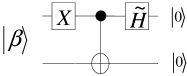
Figure 2: Quantum circuit for transforming a Bell-type state $|\beta\rangle=a|10\rangle+b|01\rangle)$ to the initial state $|00\rangle$. So, $|00\rangle=\widetilde{H}^{1}\cdot CNOT\cdot X^{1}\cdot|\beta\rangle$.

The following is an example that shows how the configuration coefficients can be addressed and the number of the configurations in the target state can be reduced through the application of the generalized Hadamard gate $\widetilde{H}$ and $C$-$\widetilde{H}$ gate. To transform the state $|\Psi_{T}\rangle=\frac{1}{\sqrt{3}}|001\rangle+\frac{1}{\sqrt{6}}|010\rangle+\frac{1}{\sqrt{2}}|100\rangle$, to the state $|000\rangle=|0\rangle^{\otimes 3}$, the gate sequence is as follows:

$$|\Psi_{T}\rangle\text{ \ }\underrightarrow{\text{ }X^{1}\text{ }}\text{ \ }|1\rangle(\frac{1}{\sqrt{3}}|01\rangle+\frac{1}{\sqrt{6}}|10\rangle)+\frac{1}{\sqrt{2}}|0\rangle^{\otimes 3}$$

$$\underrightarrow{\text{ }CNOT^{1,2}\text{ }}\text{\ \ }|1\rangle(\frac{1}{\sqrt{3}}|11\rangle+\frac{1}{\sqrt{6}}|00\rangle)+\frac{1}{\sqrt{2}}|0\rangle^{\otimes 3}$$

$$\underrightarrow{\text{ }CNOT^{2,3}\text{ }}\text{ \ }|1\rangle(\frac{1}{\sqrt{3}}|10\rangle+\frac{1}{\sqrt{6}}|00\rangle)+\frac{1}{\sqrt{2}}|0\rangle^{\otimes 3}$$

$$\underrightarrow{\text{ \ \ }C\text{-}{\widetilde{H}}^{1,2}\text{ }}\text{ \ }\frac{1}{\sqrt{2}}|100\rangle+\frac{1}{\sqrt{2}}|0\rangle^{\otimes 3}$$

$$\underrightarrow{\text{ \ \ \ \ \ }H^{1}\text{\ \ \ }}\text{ \ }|0\rangle^{\otimes 3},$$ (15)

where in the $C$-$\widetilde{H}$ operation, the $\widetilde{H}$ gate is determined by solving the following equation:

$$\widetilde{H}\left(\begin{array}[]{c}\frac{1}{\sqrt{6}}\\ \frac{1}{\sqrt{3}}\end{array}\right)=\left(\begin{array}[]{cc}2uv&u^{2}-v^{2}\\ u^{2}-v^{2}&-2uv\end{array}\right)\left(\begin{array}[]{c}\frac{1}{\sqrt{6}}\\ \frac{1}{\sqrt{3}}\end{array}\right)=\frac{1}{\sqrt{2}}\left(\begin{array}[]{c}1\\ 0\end{array}\right).$$ (16)

We set $u$ and $v$ in the unitary matrix $C$ to be real numbers since the coefficients in the target state are real. Then one can obtain the unitary matrix $C$ by solving the above equation; one obtains $u=\frac{1}{6}(3\sqrt{2}+2\sqrt{3})\sqrt{3-\sqrt{6}}$ and $v=-\sqrt{1/2-1/\sqrt{6}}$. The quantum circuit for this procedure is shown in Fig. $3$.

Figure 3: Quantum circuit for transforming the three-qubit state $|\Psi_{T}\rangle=\frac{1}{\sqrt{3}}|001\rangle+\frac{1}{\sqrt{2}}|100\rangle+\frac{1}{\sqrt{6}}|010\rangle$ to the state $|0\rangle^{\otimes 3}=|000\rangle$.

III.2 One-electron system

Let $|\Psi_{T}(n,1)\rangle$ denote the state wave function of the one-electron, $n$-spin-orbital system. If we consider all possible distributions of the electron on the $n$ spin orbitals, the dimension of the configuration space will be $\left(\begin{array}[]{c}n\\ 1\end{array}\right)=n$. We call this the complete configuration space of the one-electron system. The target state can be factorized as follows:

$$|\Psi_{T}(n,1)\rangle=c_{0}|0\rangle|\Psi_{T}(n-1,1)\rangle+c_{1}|1\rangle|0\rangle^{\otimes(n-1)},$$ (17)

where $|\Psi_{T}(n-1,1)\rangle$ is a state wave function for one electron distributed on $(n-1)$ spin orbitals. The configuration coefficients in state $|\Psi_{T}(n-1,1)\rangle$ are normalized to $1$. Also, $c_{0}$ and $c_{1}$ satisfy $|c_{0}|^{2}+|c_{1}|^{2}=1$. The relative phase between two states can be addressed by some unitary operations. We define an unitary operator $Q(n-1,1)$, such that

$$Q(n-1,1)|\Psi_{T}(n-1,1)\rangle=|0\rangle^{\otimes(n-1)}.$$ (18)

The procedure for transforming the target state to the state $|0\rangle^{\otimes n}$ can be formulated as follows:

$$|\Psi_{T}(n,1)\rangle\text{ }\underrightarrow{\text{ }X^{1}\text{ }}\text{ }c_{0}|1\rangle|\Psi_{T}(n-1,1)\rangle+c_{1}|0\rangle^{\otimes n}\qquad$$

$$\underrightarrow{\text{ }C\text{-}Q(n-1,1)^{\{1,(2,\cdots,n)\}}\text{ }}\text{ }c_{0}|1\rangle|0\rangle^{\otimes(n-1)}+c_{1}|0\rangle^{\otimes n}\qquad$$

$$\underrightarrow{\text{ }\widetilde{H}^{1}\text{ }}\text{ }|0\rangle^{\otimes n},$$ (19)

where $C$-$Q(n-1,1)^{\{1,(2,\cdots,n)\}}$ is a controlled unitary operation with the first qubit as the control qubit, and qubits $2,\cdots,n$ are the target qubit. Here, the $\widetilde{H}$ gate operates on the vector $\left(\begin{array}[]{c}c_{1}\\ c_{0}\end{array}\right)$ and transforms it to the state $\left(\begin{array}[]{c}1\\ 0\end{array}\right)=|0\rangle$. Thus the gate $\widetilde{H}$ used here is determined by solving the following equation:

$$\widetilde{H}\left(\begin{array}[]{c}c_{1}\\ c_{0}\end{array}\right)=\left(\begin{array}[]{cc}u^{\ast}v+uv^{\ast}&{u^{\ast}}^{2}-{v^{\ast}}^{2}\\ u^{2}-v^{2}&-(u^{\ast}v+uv^{\ast})\end{array}\right)\left(\begin{array}[]{c}c_{1}\\ c_{0}\end{array}\right)=\left(\begin{array}[]{c}1\\ 0\end{array}\right).$$ (20)

The quantum circuit for this procedure is shown in Fig. $4$.

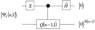
Figure 4: Quantum circuit for transforming a general state of the one-electron system $|\Psi_{T}(n,1)\rangle$ to the initial state $|0\rangle^{\otimes n}$.

The unitary operator $Q(n-1,1)$ that transforms the state $|\Psi_{T}(n-1,1)\rangle$ to the state $|0\rangle^{\otimes(n-1)}$ can be factorized similarly through the factorization of the state $|\Psi_{T}(n-1,1)\rangle$,

$$|\Psi_{T}(n-1,1)\rangle=c_{0}^{\prime}|0\rangle|\Psi_{T}(n-2,1)\rangle+c_{1}^{\prime}|1\rangle|0\rangle^{\otimes(n-2)},$$ (21)

where $|c_{0}^{{}^{\prime}}|^{2}+|c_{1}^{\prime}|^{2}=1$ and $|\Psi_{T}(n-2,1)\rangle$ is normalized to $1$. An $\widetilde{H}^{\prime}$ gate acts on the vector $\left(\begin{array}[]{c}c_{1}^{\prime}\\ c_{0}^{\prime}\end{array}\right)$ and transforms it to the state $\left(\begin{array}[]{c}1\\ 0\end{array}\right)=|0\rangle$. The $\widetilde{H}^{{}^{\prime}}$ gate can be determined by solving an equation that is similar to Eq. ($20$). We now define a unitary operator $Q(n-2,1)$, such that

$$Q(n-2,1)|\Psi_{T}(n-2,1)\rangle=|0\rangle^{\otimes(n-2)}.$$ (22)

The decomposition procedure above is repeated until the target state reaches a Bell-type state $|\Psi_{T}(2,1)\rangle=c_{0}^{\prime\prime}|01\rangle+c_{1}^{\prime\prime}|10\rangle$, whose disentanglement procedure has been explained above (Fig. $2$). The quantum circuit for this procedure of decomposing the unitary operator $Q(n-1,1)$ is shown in Fig. $5$.

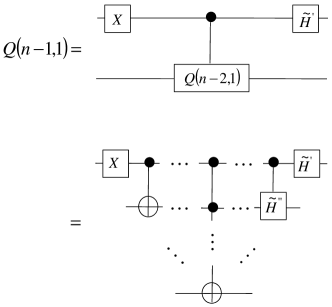
Figure 5: Quantum circuit for the decomposition of the unitary operator $Q(n-1,1)$.

From the derivation above, we can see that the preparation of the state $|\Psi_{T}(n,1)\rangle$ is reduced to the preparation of the state $|\Psi_{T}(2,1)\rangle$, which is solved above as shown in Fig. $2$. The Toffoli gate, which is also known as the “controlled-controlled-not” gate, appears when implementing this recursive procedure. We will discuss the simplification of the Toffoli gates into CNOT gates in Sec. IV. The scaling of the algorithm in terms of the number of CNOT and single-qubit gates is analyzed in Sec. V.

States in the incomplete configuration space of the one-electron system are easier to prepare than those in the complete configuration space, since the former can be reduced to states in a complete configuration space of lower dimension.

III.3 $m$-electron system

For the $m$-electron system, it becomes more difficult to prepare the target state than for the one-electron system. We apply a recursive approach to solve this problem based on the following facts:

(1) Any state of the one-electron system can be prepared [as shown in Sec. I​I​I. B.]

(2) An arbitrary state $|\Psi_{T}(p,p-1)\rangle$ can be prepared. [By applying $X^{\otimes p}$ gates, the state is transformed to $|\Psi_{T}(p,1)\rangle$, which is a one-electron state.]

We now define a unitary operator $U(n,m)$ such that:

$$U(n,m)|\Psi_{T}(n,m)\rangle=|0\rangle^{\otimes n}.$$ (23)

A quantum circuit for $U(n,m)$ can be obtained through the decomposition of the state $|\Psi_{T}(n,m)\rangle$ as follows.

Any arbitrary target state [Eq. ($10$)] can be rewritten in the following way:

$$|\Psi_{T}\rangle=\sum_{i=1}^{N_{0}}k_{0,i}|0\rangle|\psi_{i}\rangle+\sum_{j=1}^{N_{1}}k_{1,j}|1\rangle|\psi_{j}\rangle,$$ (24)

where the state is divided in two parts: one of them lies in the subspace where the first qubit is in state $|0\rangle$ (we call this the $|0\rangle$ subspace); the other part lies in the subspace where the first qubit is in state $|1\rangle$ (we call this the $|1\rangle$ subspace). Also, $N_{0}$ is the dimension of the $|0\rangle$ subspace and $N_{1}$ is the dimension of the $|1\rangle$ subspace. The target state can be factorized as follows:

$$|\Psi_{T}(n,m)\rangle=c_{0}|0\rangle|\Psi_{T}(n-1,m)\rangle+c_{1}|1\rangle|\Psi_{T}(n-1,m-1)\rangle.$$ (25)

The coefficients $c_{0}$ and $c_{1}$ are calculated as:

$$|c_{0}|^{2}=\sum_{i=1}^{N_{0}}|k_{0,i}|^{2},\qquad|c_{1}|^{2}=\sum_{j=1}^{N_{1}}|k_{1,j}|^{2},$$ (26)

where $|c_{0}|^{2}+|c_{1}|^{2}=1$. We now define unitary operators $U(n-1,m)$ and $U(n-1,m-1)$ such that

$$U(n-1,m)|\Psi_{T}(n-1,m)\rangle=|0\rangle^{\otimes(n-1)},$$ (27)

$$U(n-1,m-1)|\Psi_{T}(n-1,m-1)\rangle=|0\rangle^{\otimes(n-1)}.$$ (28)

The relative phase between two configurations can be included in these unitary operators. Then the target state can be transformed to the initial state $|0\rangle^{\otimes n}$ in the following way:

$$|\Psi_{T}(n,m)\rangle\text{ }\underrightarrow{\text{ }X^{1}\text{ }}\text{\ }c_{0}|1\rangle|\Psi_{T}(n-1,m)\rangle$$

$$+c_{1}|0\rangle|\Psi_{T}(n-1,m-1)\rangle$$

$$\underrightarrow{\text{ \ }U(n-1,m-1)\text{ \ }}$$

$$c_{0}|1\rangle U(n-1,m-1)|\Psi_{T}(n-1,m)\rangle+c_{1}|0\rangle^{\otimes n}$$

$$\underrightarrow{\text{ \ }{C}\text{{-}}{U(n-1,m-1)^{-1}}^{\{1,(2,\cdots,n)\}}\text{ \ }}\text{ }$$

$$c_{0}|1\rangle|\Psi_{T}(n-1,m)\rangle+c_{1}|0\rangle^{\otimes n}$$

$$\underrightarrow{\text{ \ }C\text{-}U(n-1,m)^{\{1,(2,\cdots,n)\}}\text{ \ }}$$

$$c_{0}|1\rangle|0\rangle^{\otimes(n-1)}+c_{1}|0\rangle^{\otimes n}$$

$$\underrightarrow{\text{ \ }\widetilde{H}^{1}\text{ \ }}\text{ }|0\rangle^{\otimes n}.$$ (29)

The quantum circuit for this procedure is shown in Fig. $6$.

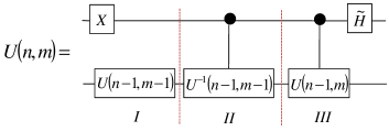
Figure 6: Quantum circuit for transforming a general state $|\Psi_{T}(n,m)\rangle$ of the $m$-electron system to the initial state $|0\rangle^{\otimes{n}}$.

The unitary operators $U(n-1,m)$ and $U(n-1,m-1)$ that transform the states $|\Psi_{T}(n-1,m)\rangle$ and $|\Psi_{T}(n-1,m-1)\rangle$ to the state $|0\rangle^{\otimes(n-1)}$ can be decomposed through the decomposition of the states $|\Psi_{T}(n-1,m)\rangle$ and $|\Psi_{T}(n-1,m-1)\rangle$. For example, for the operator $U(n-1,m-1)$, we have:

$$|\Psi_{T}(n-1,m-1)\rangle = c_{0}^{\prime}|0\rangle|\Psi_{T}(n-2,m-1)\rangle$$ (30)

$$+c_{1}^{\prime}|1\rangle|\Psi_{T}(n-2,m-2)\rangle.$$

Define unitary operators $U(n-2,m-1)$ and $U(n-2,m-2)$ such that

$$U(n-2,m-1)|\Psi_{T}(n-2,m-1)\rangle=|0\rangle^{\otimes(n-2)},$$ (31)

$$U(n-2,m-2)|\Psi_{T}(n-2,m-2)\rangle=|0\rangle^{\otimes(n-2)}.$$ (32)

The quantum circuit for $U(n-1,m-1)$ is similar to the circuit in Fig. $6$, where $n$ and $m$ in the unitary operators on the bottom line of the circuit are replaced by $(n-1)$ and $(m-1)$, respectively.

One can repeat this procedure until reaches a one-electron state $|\Psi_{T}(p,1)\rangle$, where $2\leq p\leq n$, or a $|\Psi_{T}(p,p-1)\rangle$ state, which is solved as we discussed above. In each iteration, the unitary operators can be decomposed into the circuits that have the same structure as shown in Fig. $6$. Such that the problem of transforming a general $m$-electron, $n$-spin-orbital state $|\Psi_{T}(n,m)\rangle$ to the initial state $|0\rangle^{\otimes n}$ can be solved. This algorithm also works for systems of different numbers of the electrons. The simplification of the twofold controlled unitary operations and the scaling of the algorithm are discussed in Secs. I​V and V.

IV Simplification of the two-fold controlled gates

Because controlled gates appear inside the controlled operations in Sec. I​I​I, the twofold controlled gates appear in the implementation of the recursive procedure for state preparation. For the simplest twofold controlled gates, the Toffoli gate toff , which is also known as the “controlled-controlled-not” gate, in general, six CNOT gates are needed for implementing a three-qubit Toffoli gate barenco . However, if the input state for the quantum circuit is known, then the operation of a given unitary operator on all orthogonal states is immaterial. In such cases the unitary operator is said to be incompletely specified shende . Thus, there exists more than one quantum circuit for performing such an operation. So, one can select a simpler circuit in order to reduce the number of gates. Based on this, we will now simplify the two-fold controlled gates in the algorithm.

In our algorithm, the problem of preparing an $n$-qubit state is reduced to the problem of preparing some simpler states [i.e., for one-electron system, the problem is reduced to the preparation of a Bell-type state; for a general $m$-electron system, the problem is reduced to the preparation of states $|\Psi_{T}(p,1)\rangle$ and $|\Psi_{T}(p,p-1)\rangle$]. We will show that the twofold controlled gates that appear in each step of this recursive procedure can be simplified to onefold controlled gates by just turning off the operation of the first control qubit. The recursive approach for constructing the quantum circuit leads to another advantage: for the controlled operations, it provides a way that makes the shortest distance between the control qubit and the target qubit since the controlled operations are simplified in each step while expanded to one more qubit.

For the one-electron system, plugging the circuit for $Q(n-1,1)$ shown in Fig. $5$ into Fig. $4$, the quantum circuit for transforming the target state $|\Psi_{T}(n,1)\rangle$ to the state $|0\rangle^{\otimes n}$ is shown in the top part of Fig. $7$. The quantum circuit has the following structure: from right to left, the input state is $|0\rangle^{\otimes n}$; an $\widetilde{H}$ gate operates on the first qubit and followed by a $C$-$\widetilde{H}^{{}^{\prime}}$ gate. After the application of these two gates, the basis vectors that span the state on the two control qubits are $\{|00\rangle$, $|10\rangle$, $|11\rangle\}$. The basis vector $|01\rangle$ does not appear, such that the two-fold controlled gates following these operations are incompletely specified. From right to left, taking $|0\rangle^{\otimes n}$ as the input state, the basis vectors that appear in the state of the qubits change as follows:

$$|0\rangle^{\otimes n}\text{ }\underrightarrow{\widetilde{H}^{1}}\text{ }\left\{\begin{array}[]{c}|0\rangle|0\rangle^{\otimes(n-1)}\\ |1\rangle|0\rangle^{\otimes(n-1)}\end{array}\right\}\underrightarrow{{C\text{{-}}\widetilde{H}^{{}^{\prime}}}^{1,2}}\left\{\begin{array}[]{c}|0\rangle|0\rangle|0\rangle^{\otimes(n-2)}\\ |1\rangle|0\rangle|0\rangle^{\otimes(n-2)}\\ |1\rangle|1\rangle|0\rangle^{\otimes(n-2)}\end{array}\right\}\underrightarrow{C\text{{-}}{Q(n-2,1)^{-1}}^{(1,2),(3,\cdots,n)}}\left\{\begin{array}[]{c}|0\rangle|0\rangle|0\rangle^{\otimes(n-2)}\\ |1\rangle|0\rangle|0\rangle^{\otimes(n-2)}\\ |1\rangle|1\rangle Q(n-2,1)^{-1}|0\rangle^{\otimes(n-2)}\end{array}\right\}.$$ (33)

The twofold controlled unitary operator $C$-${Q^{-1}(n-2,1)}^{(1,2),(3,\cdots,n)}$ is incompletely specified. Here the use of $C$-${Q^{-1}(n-2,1)}^{(1,2),(3,\cdots,n)}$ instead of $C$-$Q(n-2,1)^{(1,2),(3,\cdots,n)}$ is because we let the gates operate to the right. As a result, it can be simplified to $C$-${Q^{-1}(n-2,1)}^{2,(3,\cdots,n)}$. This simplification can be repeated in each recursive step until the state reaches a Bell-type state $|\Psi_{T}(2,1)\rangle$. The simplified quantum circuit is shown in the bottom part of Fig. $7$.

Figure 7: Top quantum circuit for the recursive procedure to transform the state $|\Psi_{T}(n,1)\rangle$ to the initial state $|0\rangle^{\otimes n}$. It has two one-fold control operations and one two-fold operation in the middle. The bottom circuit shows its simplified version, without two-fold operations.

For the $m$-electron system, each of the three unitary operators in the bottom line of the quantum circuit in Fig. $6$ can be decomposed into the circuit that has the same structure as that of $U(n,m)$. The circuit in Fig. $6$ is divided in three parts. The two-fold controlled unitary operator in the controlled operations in parts $I\!I$ and $I\!I\!I$ will appear when they are expanded to one more qubit. Taking the state $|0\rangle^{\otimes n}$ as the input state, from right to left, following the operation of the circuit, the basis vectors that appear in the state of the qubits change in the same way as that of the one-electron system. These twofold controlled unitary operators in parts I​I and I​I​I of Fig. $6$ are incompletely specified. For quantum circuit $U(n-1,m-1)$ that acts on qubits $2,\cdots,n,$ in part I of Fig. $6$, the twofold controlled unitary operators may appear when the circuit is decomposed one more step. From left to right in Fig. $6$, after the circuit in part I operates on the target state $|\Psi_{T}(n,m)\rangle$, the target state is transformed to $c_{1}|1\rangle U(n-1,m-1)|\Psi_{T}(n-1,m)\rangle+c_{0}|0\rangle^{\otimes n}$. This intermediate state can be divided in two branches: the $|0\rangle$ branch, $|0\rangle^{\otimes n},$ and the $|1\rangle$ branch, $|1\rangle U(n-1,m-1)|\Psi_{T}(n-1,m)\rangle$. For the $|1\rangle$ branch, the operation of $U(n-1,m-1)$ that acts on qubits $2,\cdots,n$, will be cancelled with the controlled operation $C$-$U^{-1}(n-1,m-1)$ in part I​I. For the $|0\rangle$ branch of the state, the state on qubits $2,\cdots,n,$ is $|0\rangle^{\otimes(n-1)}$, and it acts as the input state for the circuit $U(n-1,m-1)$ from right to left. Then the unitary operator $U(n-1,m-1)$ has the same structure and input state as that of $U(n,m)$ we discussed above. The twofold controlled unitary operators in $U(n-1,m-1)$ (part I of Fig. $6$) are also incompletely specified.

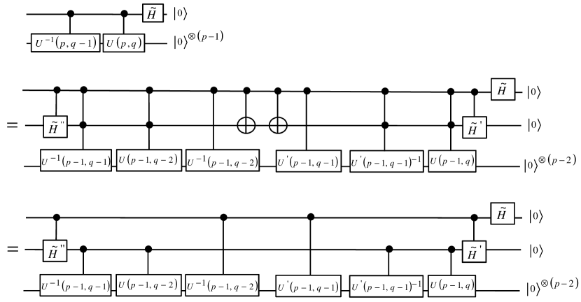
Figure 8: Quantum circuit for two controlled unitary operators $C$-$U(p,q)$ and $C$-$U(p,q-1)$ and their simplified versions. The two unitary operators in the top circuit are expanded in the second circuit, which is simplified in the bottom circuit.

According to the analysis above, the unitary operator $U(n-1,m-1)$ has the same structure as the circuit for $U(n,m)$, with state $|0\rangle^{\otimes(n-1)}$ as the input state. The twofold controlled unitary operators in the controlled unitary operators in $U(n-1,m-1)$ and $U(n,m)$ are incompletely specified. A general form of the structure of the controlled unitary operators is shown in Fig. $8$. The twofold controlled unitary operators in them are incompletely specified, and can be simplified by just turning off the operation of the first control qubit as shown in Fig. $8$. Then all the twofold controlled gates in the circuit can be simplified.

V Scaling of the algorithm

In this section, we analyze the scaling of the algorithm for state preparation. The cost of a quantum algorithm is usually given by the number of CNOT gates used. Here we count all the twofold controlled gates as twoqubit gates since all twofold controlled gates can be simplified to onefold controlled gates, as shown in Sec. V​I​I.

In the one-electron system, for states in the complete configuration space, the scaling of the algorithm is derived as follows: let $N(n,1)$ denote the total number of gates, including both CNOT and single-qubit gates, needed to prepare the target state $|\Psi_{T}(n,1)\rangle$ from the initial state $|0\rangle^{\otimes n}$. From the quantum circuit shown in Fig. $7$, one can see that there are four gates (a $\widetilde{H}$ gate is composed of three gates: $C^{{\dagger}}$, $C$, and NOT gates) on each line of the circuit, except the last line, which has one gate. Therefore the total number of gates is $N(n,1)=4n-3$. The number CNOT gates can be derived as follows: denote $N_{\text{CNOT}}(n,1)$ as the number of CNOT gates. From Fig. $7$, we have $N_{\text{CNOT}}(n,1)-N_{\text{CNOT}}(n-1,1)=2$(by adding one control qubit, one obtains two more controlled gates, a CNOT gate and a $C$-$\widetilde{H}$ gate). Then keep this decomposition procedure until $n=2$, we obtain $N_{\text{CNOT}}(n,1)=2n-3$. This is the upper bound of the number of CNOT gates for preparing a state in the one-electron system, since a target state in the incomplete configuration space can be reduced to a state in the complete configuration space with fewer qubits.

For the two-electron system, denote $N(n,2)$ as the number of gates needed to prepare the target state $|\Psi_{T}(n,2)\rangle$from the $|0\rangle^{\otimes n}$. Apply the decomposion procedure in Fig. $6$ until $n=2$, and using the result from the one-electron system that $N(n,1)=4n-3$, we obtain $N(n,2)=4n^{2}-10n+6$. The number of CNOT gates can be derived as follows: let $N_{\text{CNOT}}(n,2)$ represent the number of CNOT gates needed to prepare the target state $|\Psi_{T}(n,2)\rangle$. Apply the procedure in Fig. $6$ until $n=2$, and using the result from the one-electron system, we obtain $N_{\text{CNOT}}(n,2)=2n^{2}-6n+4$.

The scaling for preparing a general state of the $m$-electron system is derived as follows: denote $N(n,m)$ as the maximum number of gates, including both CNOT and single-qubit gates, needed to prepare the state of given values of $n$ and $m$. We should stress that all two-fold controlled gates can be simplified to one-fold controlled gates (see Sec. IV). Looking at Fig. $6$ and assuming that each block in it contains the maximum number of gates possible for the size of the block, we have:

$$N(n,m)=2N(n-1,m-1)+N(n-1,m)+2,$$ (34)

The first order derivative of $N(n,m)$ with respect to $n$, where $N$ and $n$ are integers and the derivative is taken accordingly, is:

$$\frac{dN(n,m)}{dn} = \frac{N(n,m)-N(n-1,m)}{n-(n-1)}$$ (35)

$$= 2N(n-1,m-1)+2.$$

Using Eq. ($34$), the second order derivative of $N(n,m)$ is:

$$\frac{d^{2}N(n,m)}{dn^{2}} = \frac{d}{dn}\left(\frac{dN(n,m)}{dn}\right)$$ (36)

$$= \frac{d}{dn}\left(2N(n-1,m-1)\right)$$

$$= 2^{2}N(n-2,m-2)+2^{2},$$

After $(m-1)$ steps of taking the derivative of $N(n,m)$, we have:

$$\frac{d^{m-1}N(n,m)}{dn^{m-1}}=2^{m-1}N(n-m+1,1)+2^{m-1}.$$ (37)

Using the scaling law given above for the one-electron case, i.e. $N(n-m+1,1)=4n-4m+1$, we find that:

$$\frac{d^{m}N(n,m)}{dn^{m}}=2^{m-1}\text{ x }4=2^{m+1}.$$ (38)

We can now obtain the scaling behavior for preparing a general pure state of the $m$-electron, $n$-spin-orbital system by integrating Eq. ($38$) $m$ times:

$$N(n,m)\propto\frac{2^{m+1}}{m!}n^{m},$$ (39)

which scales polynomially with $n$, the number of qubits in the system. Since $N(n,m)$ is the maximum number of gates needed to prepare a state with given values of $n$ and $m$, the scaling in Eq. ($39$) can be thought of as the upper bound of the number of gates needed to prepare the target state $|\Psi_{T}(n,m)\rangle$ from $|0\rangle^{\otimes n}$. The number of $C$-$\widetilde{H}$ gates is the majority of the circuit, e.g., as shown in Fig. $8$; a $C$-$\widetilde{H}$ gate is composed of two single-qubit gates, $C^{{\dagger}}$ and $C$, and a CNOT gate. The number of CNOT gates is comparable with the number single-qubit gates, both scaling as $O(2^{m}n^{m}/m!)$.

We now compare the scaling $O(2^{m}n^{m}/m!)$ with $O(2^{n})$, the number of gates needed to prepare an arbitrary $n$-qubit state. We look for the condition that makes $2^{m}n^{m}/m!$ smaller than $2^{n}$. Using the Sterling approximation we have:

$$\frac{2^{m}}{m!}n^{m}\approx\frac{(2n)^{m}}{(\frac{m}{e})^{m}}=\left(\frac{2en}{m}\right)^{m}.$$ (40)

Then the following equations need to be satisfied:

$$\left(\frac{2en}{m}\right)^{m}\leq 2^{n},$$ (41)

$$m\log_{2}\left(\frac{2en}{m}\right)\leq n,$$ (42)

$$m\log_{2}n<n.$$ (43)

One can see that if $m<n/\log_{2}n$, our algorithm is more efficient than the algorithms mentioned in Refs. shende and mott . Then we compare the scaling of our algorithm with another algorithm introduced by Ortiz et al. ortiz , $O(N^{2}n^{2})$. Assuming $N\sim\left(\begin{array}[]{c}n\\ m\end{array}\right)$, then looking for the condition that makes $2^{m}n^{m}/m!$ smaller than $N^{2}n^{2}$, we have:

$$\frac{2^{m}}{m!}n^{m}<\left(\begin{array}[]{c}n\\ m\end{array}\right)^{2}n^{2}\approx\left(\frac{n^{m}}{m^{m}}\right)^{2}n^{2},$$ (44)

$$2^{m}<\left(\frac{n}{m}\right)^{m}n^{2}.$$ (45)

One can see that as long as $n>2m$, our algorithm is more efficient than the algorithm in Ref. ortiz . In quantum chemistry, usually $n\gg m$, i.e., many more orbitals are needed to describe a given number of electrons. The number of orbitals needed to describe a fixed number of electrons depends on the accuracy of the calculation and the specific states that are investigated. For example, to study the highly excited states of a molecular system, more orbitals are needed than in study of the ground state. The number of orbitals needed and the number of electrons are therefore independent. So our algorithm gives an efficient way of preparing a general state for accurate simulation of a wide range of molecular systems.

VI Application to some molecular systems

In this section, we apply the algorithm to two molecular systems: the hydrogen molecule and the water molecule. We prepare the multi-configurational self-consistent field (MCSCF) whf wave function of these two molecules. The MCSCF wave function is a linear combination of a number of CSFs, where each CSF is a symmetry-adapted linear combination of electron configurations.

The state function is a CSF, i.e., it is an eigen-function of the operators $\hat{L}^{2}$ and $\hat{S}^{2}$, where $\hat{L}$ and $\hat{S}$ are the orbital angular momentum operator and the spin operator, respectively. In quantum chemistry, one is usually most interested in the spin-states, i.e., the states that have certain spin multiplicity, of the molecular system. For molecules that have space symmetry, the electronic states of the molecule can be categorized into different irreducible representations of their point group. One only needs to perform calculations on states that belong to a certain irreducible representation. Considering these effects, the number of configurations in the state function can be drastically below the size of the Hilbert space. The state function is spanned only in a subspace of dimension much smaller than $\left(\begin{array}[]{c}n\\ m\end{array}\right)$. Therefore many configurations do not appear in the decomposition procedure shown in Eq. ($24$), where the state function is decomposed into a $|0\rangle$ branch and a $|1\rangle$ branch. As a result, fewer gates are needed to prepare the state than the conservative estimate given in Sec. V. Note that the algorithm itself is not simplified in any way when considering the symmetries of the molecule.

VI.1 Hydrogen molecule

We use the MCSCF method with the cc-pVDZ basis set dunning to study the electronic structure of the hydrogen molecule. This gives $20$ spin orbitals. Two electrons are distributed on these orbitals with the restriction of the spin multiplicity of the spin state. Considering the $D_{\infty h}$ symmetry of the molecule, the ground state of H₂ is ${}^{1}\Sigma_{g}^{+}$ (${}^{1}\Sigma_{g}^{+}$ is the Mulliken symbol that is used to label many-electron states; $\Sigma$, $g$, $+$, and the superscript “$1$” represents angular momentum, parity, symmetry with respect to a vertical mirror plane perpendicular to the principal axis, and the spin multiplicity).

For $20$ qubits, the dimension of the whole Hilbert space is $2^{20}\sim 10^{6}$; for a fixed number of electrons, the two-electron, $20$-spin-orbital system is of dimension $\left(\begin{array}[]{c}20\\ 2\end{array}\right)=190$; considering the spin multiplicity and the space symmetry, the ground state MCSCF wave function is composed of at most $16$ electron configurations. We can see that by considering the spin multiplicity and the space symmetry, the state space is drastically reduced.

To prepare the state function in the full space of $\left(\begin{array}[]{c}20\\ 2\end{array}\right)$ using our state preparation algorithm, we need roughly $800$ CNOT gates. To prepare the MCSCF wave function that is composed of $16$ electron configurations, by performing a numerical calculation, we found that only $37$ CNOT gates and $31$ single-qubit gates are needed in total. This number, $37$, is well below the conservative estimate of about $800$ CNOT gates needed to prepare an arbitrary two-electron, $20$-spin-orbital state.

VI.2 Water molecule

For another example, the water molecule H₂O, we use the MCSCF method with the cc-pVDZ basis set dunning . For the ground state, considering the $C_{2V}$ symmetry of the water molecule, the Hartree-Fock wave function of the H₂O molecule is:

$$(1a_{1})^{2}(2a_{1})^{2}(1b_{2})^{2}(3a_{1})^{2}(1b_{1})^{2}\text{ .}$$ (46)

The ground state of H₂O is the ${}^{1}A_{1}$ state. We apply a complete active space (CAS) type MCSCF method in order to reduce the cost of the calculation: the first two $a_{1}$ orbitals are frozen, the active space consists of the $3a_{1}$-$6a_{1}$ orbitals, $1b_{1}$, $1b_{2}$ and $2b_{2}$ orbitals. So there are $14$ spin orbitals and $6$ electrons in the active space.

For $14$ qubits, the dimension of the whole Hilbert space is $2^{14}\sim 10^{4}$; the six-electron, $14$-spin-orbital system is of dimension $\left(\begin{array}[]{c}14\\ 6\end{array}\right)=3003$. To prepare the state function in this space using our algorithm, we need roughly $670000$ CNOT gates, which is larger than $2^{14}\sim 10^{4}$, the number of CNOT gates needed to prepare a state in the full Hilbert space of $14$ qubits. Considering the spin multiplicity and the space symmetry of the molecule, the ground state MCSCF wave function is composed of $152$ electron configurations. To prepare the state function using our state preparation algorithm, performing the numerical calculation, we found that we need $1472$ CNOT gates and $1146$ single qubit gates. This represents a considerable and remarkable reduction of over $3$ orders of magnitude in the number of CNOT gates (from $\sim 670000$ to $\sim 1470$) needed to prepare an arbitrary six-electron, $14$-spin-orbital state.

From these two examples, we can see that if the number of electrons is comparable to the number of spin orbitals, the number of CNOT gates needed to prepare the corresponding state increases very fast. The algorithm is no longer efficient. However, in quantum chemistry, the number of orbitals needed for simulation purposes is usually much larger than the number of electrons. In the case of $n\gg m$, our algorithm provides an efficient way in preparing states of molecular systems, as demonstrated in the example of the hydrogen molecule above.

VII conclusion

In this paper, we present an efficient quantum algorithm for preparing a pure molecular-system-like state. The simulated system lies in the Fock space of a given number $m$ of electrons and $n$ spin orbitals on a quantum computer. The state wave function is a configuration state function and is entangled in general. In general this is to prepare a pure state in the combinatorial space $\left(\begin{array}[]{c}n\\ m\end{array}\right)$ after the Jordan-Wigner transformation.

In our algorithm, instead of starting from an initial state and transforming it to the target state, we start from the target state and transform it to the initial state. Then by inverting the quantum circuit sequence, we obtain the circuit for preparing the target state. A recursive procedure is employed for solving this problem. The twofold controlled gates that appear in each step of the recursive procedure can be simplified to one-fold controlled gates by turning off the operation of the first control qubit, since these gates are incompletely specified. We show that at most $O(2^{m+1}n^{m}/m!)$ gates, including both CNOT and single-qubit gates, are needed to prepare a general state of the $m$-electron, $n$-spin-orbital system, which scales polynomially with $n$. The number of CNOT gates scales as $O(2^{m}n^{m}/m!)$. This state preparation algorithm works for systems of arbitrary number of electrons, but the number of CNOT gates needed will increase exponentially if the number of electrons $m$ is proportional to the number of spin orbitals $n.$

As examples, we have simulated our state preparation algorithm for the hydrogen and water molecules. In these two specific cases we analyzed, using the known symmetries of the molecules, we found that the number of CNOT gates is reduced by up to $3$ orders of magnitude. This provides a remarkable simplification to this type of problems.

Note added.—In the final stages of preparing this paper, we became aware of a paper that outlined a quantum algorithm for the preparation of many-particle states on a lattice guziksp , in which the state is prepared in the first-quantized representation, while ours is in the second-quantized representation. We give an explicit and elaborate solution to the problem and in a very different way.

- (1) T. Helgaker, P. Jorgenson, and J. Olsen, Molecular Electronic-Structure Theory (Wiley, Chichester, 2000).
- (2) L. Thögersen, and J. Olsen, Chem. Phys. Lett. 393, 36 (2004).
- (3) R. Feynman, Int. J. Theor. Phys. 21, 467 (1982).
- (4) S. Lloyd, Science 273, 1073 (1996).
- (5) C. Zalka, Proc. R. Soc. London. Ser. A 454, 313 (1998).
- (6) D. S. Abrams and S. Lloyd, Phys. Rev. Lett. 83, 5162 (1999).
- (7) D. A. Lidar and H. Wang, Phys. Rev. E. 59, 2429 (1999).
- (8) E. Manousakis, J. Low Temp. Phys., 126, 1501 (2002).
- (9) A. Aspuru-Guzik, A. D. Dutoi, P. J. Love, and M. Head-Gordon, Science 309, 1704 (2005).
- (10) H. F. Wang, S. Kais, A. Aspuru-Guzik, and M. R. Hoffmann, Phys. Chem. Chem. Phys. 10, 5388 (2008).
- (11) I. Kassal, S. P. Jordan, P. J. Love, M. Mohseni, and A. Aspuru-Guzik, Proc. Natl. Acad. Sci. U.S.A. 105, 18681 (2008).
- (12) A. Yu. Smirnov, S. Savel’ev, L. G. Mourokh, and F. Nori, EPL 80 67008 (2007).
- (13) I. M. Buluta and F. Nori (unpublished).
- (14) J. Q. You and F. Nori, Phys. Today 58 (11), 42 (2005).
- (15) P. Jordan and E. Wigner, Z. Phys. 47, 631 (1928).
- (16) V. V. Shende and I. L. Markov, Quantum Inf. Comput. 5, 49 (2005).
- (17) M. Möttönen, J. J. Vartiainen, V. Bergholm, and M. M. Salomaa, Quantum. Inf. Comput. 5, 467 (2005).
- (18) V. Bergholm, J. J. Vartiainen, M. Möttönen, and M. M. Salomaa, Phys. Rev. A 71, 052330 (2005).
- (19) A. N. Soklakov and R. Schack, Phys. Rev. A 73, 012307 (2006).
- (20) G. Ortiz, J. E. Gubernatis, E. Knill and R. Laflamme, Phys. Rev. A 64, 022319 (2001).
- (21) G. Vidal and C. M. Dawson, Phys. Rev. A 69, 010301(R) (2004).
- (22) F. Vatan and C. Williams, Phys. Rev. A 69, 032315 (2004).
- (23) V. V. Shende, I. L. Markov, and S. S. Bullock, Phys. Rev. A 69, 062321 (2004).
- (24) J. Zhang, J. Vala, S. Sastry and K. B. Whaley, Phys. Rev. Lett. 93, 020502 (2004).
- (25) J. J. Vartiainen, M. Möttönen, and M. M. Salomaa, Phys. Rev. Lett. 92, 177902 (2004).
- (26) M. Möttönen, J. J. Vartiainen, V. Bergholm, and M. M. Salomaa, Phys. Rev. Lett. 93, 130502 (2004).
- (27) V. V. Shende, S. S. Bullock, and I. L. Markov, IEEE Trans. on Comput.-Aided Des. 25, 1000 (2006).
- (28) R. R. Tucci, e-print arXiv:quant-ph/9902062.
- (29) E. Fredkin and T. Toffoli, Int. J. Theor. Phys. 21, 219 (1982).
- (30) A. Barenco, C. H. Bennett, R. Cleve, D. P. Di Vincenzo, N. Margolus, P. Shor, T. Sleator, J. A. Smolin, and H. Weinfurter, Phys. Rev. A 52, 3457 (1995).
- (31) T. H. Dunning, Jr., J. Chem. Phys. 90, 1007 (1989).
- (32) N. J. Ward, I. Kassal, and A. Aspuru-Guzik, e-print arXiv:0812.2681, (2008).