Spectral properties of non-conservative multichannel SUSY partners of the zero potential

Abstract

Spectral properties of a coupled $N\times N$ potential model obtained with the help of a single non-conservative supersymmetric (SUSY) transformation starting from a system of $N$ radial Schrödinger equations with the zero potential and finite threshold differences between the channels are studied. The structure of the system of polynomial equations which determine the zeros of the Jost-matrix determinant is analyzed. In particular, we show that the Jost-matrix determinant has $N2^{N-1}$ zeros which may all correspond to virtual states. The number of bound states satisfies $0\leq n_{b}\leq N$. The maximal number of resonances is $n_{r}=(N-1)2^{N-2}$. A perturbation technique for a small coupling approximation is developed. A detailed study of the inverse spectral problem is given for the $2\times 2$ case.

, ,

1 Introduction

Almost all low-energy collisions of microparticles with an internal structure (i.e., atom-atom, nucleus-nucleus etc) include inelastic processes such as excitations of internal degrees of freedom of colliding particles or processes with rearrangements of their constituent parts. These processes can be described by a matrix (more precisely multichannel) Schrödinger equation with a local matrix potential [1, 2]. One may be interested in both direct and inverse scattering problems for this equation. The method of SUSY transformations is known as a powerful tool for solving both types of problems for a single-channel Schrödinger equation [3]. Nowadays, the first attempt to generalize the method for a coupled-channel Schrödinger equation with different thresholds is given in [4, 5]. This attempt is based on a non-conservative SUSY transformation (contrary to [6, 7]), i.e. a SUSY transformation that does not preserve a boundary behavior of solutions. The main advantage of such transformations is a possibility to obtain multichannel potentials with a non-trivial coupling starting from the zero potential.

The present work is aimed at the investigation of spectral properties of these SUSY potentials. Our approach is based on an analysis of the Jost matrix. In the non-relativistic scattering theory the Jost matrix plays a fundamental role similar to the scattering matrix. The zeros of the Jost-matrix determinant define positions of the bound/virtual states and resonances [1, 2]. Therefore, studying the zeros of the Jost-matrix determinant allows one to analyze the spectrum of the model. A closed analytical expression of the Jost matrix, as well as potential, resulting from a non-conservative SUSY transformation of the zero potential is obtained in [4]. The analysis of spectral properties for such potentials was not presented up to now despite the fact that the Jost matrix is well known [8]. This may be explained by the fact that the spectrum of the potential after a non-conservative SUSY transformation changes essentially and to find these changes one has to find all the zeros of the Jost-matrix determinant. More precisely, no one spectral point of the initial Hamiltonian belongs to the spectrum of the transformed Hamiltonian. As a result, a supersymmetry algebra, which is always present in the case of conservative SUSY transformations, cannot actually be constructed here and the word ’SUSY transformation’ is only a formal heritage from the previous conservative case [6, 7].

The principal point of this paper is to show that the qualitative behavior of the spectrum of (non-conservative) SUSY partners of the vanishing multichannel potential with threshold differences may be studied for an arbitrary number of channels, $N$. We think this is a very strong result, since even for the case $N=2$ the full analysis of the spectrum is a very complicated problem [8, 10, 11]. The main reason for this is an extremely rapid growth of the order of an algebraic equation defining the spectrum with the growth of the number of channels.

The paper is organized as follows. We start with preliminaries, where we give basic definitions and equations. Section 3 is devoted to the analysis of the number of bound states resulting from a non-conservative SUSY transformation of the zero potential as a function of the parameters defining the transformation. This analysis is based on the study of the properties of the eigenvalues of the Jost matrix. Following similar lines we analyze the possible number of virtual states in section 4. Once the bound and virtual states are analyzed we can formulate conditions under which resonances may appear; this is made in section 5. The behavior of the Jost-matrix determinant zeros is studied in section 6 in the approximation of a weak coupling between channels. In section 7 we deal with the particular two-channel case. In this case we express parameters of the potential in terms of zeros of the Jost-matrix determinant, i.e. solve an inverse spectral problem. The main results are summarized in the conclusion.

2 Preliminaries

Let us first summarize the notations used below for coupled-channel scattering theory [1, 2, 9]. We consider a system of coupled radial Schrödinger equations for the $s$-waves that in reduced units reads

$$H\psi(k,r)=K^{2}\psi(k,r),\quad r\in(0,\infty)$$ (1)

with

$$H=-\mathbf{1}\frac{d^{2}}{dr^{2}}+V(r),$$ (2)

where $r$ is the radial coordinate, $V(r)$ is an $N\times N$ real symmetric matrix, $\mathbf{1}$ is the unit matrix, and $\psi$ may be either a matrix-valued or a vector-valued solution. By $k$ we denote a point in the space ${\mathbb{C}}^{N}$, $k=\left\{k_{1},\ldots,k_{N}\right\}$, $k_{i}\in\mathbb{C}$. A diagonal matrix with non-vanishing entries $k_{i}$ is written as $K=\mbox{diag}(k)=\mbox{diag}(k_{1},\ldots,k_{N})$. The complex wave numbers $k_{i}$ are related to the center-of-mass energy $E$ and the channel thresholds $\Delta_{1},\dots,\Delta_{N}$, which are supposed to be different from each other, $\Delta_{i(\neq j)}\neq\Delta_{j}$, by

$$k_{j}^{2}=E-\Delta_{j}\,,\qquad\Delta_{1}=0\,.$$ (3)

We assume here that $\Delta_{1}=0$ and the different channels have equal reduced masses, a case to which the general situation can always be formally reduced [2].

Let us recall basic definitions from SUSY quantum mechanics [3, 4, 5, 6, 7]. It is known that the solutions of the initial Schrödinger equation (1) may be mapped into the solutions of the transformed equation with help of the differential-matrix operator

$$\tilde{\psi}(k,r)=L\psi(k,r)=\left[-\mathbf{1}\frac{d}{dr}+U(r)\right]\psi(k,r)\,.$$ (4)

The transformed Schrödinger equation has form (1) with a new potential

$$\tilde{V}(r)=V(r)-2U^{\prime}(r)\,.$$ (5)

Matrix $U$ is called superpotential

$$U(r)=\eta^{\prime}(r)\eta^{-1}(r)\,,$$ (6)

and expressed in terms of a matrix solution $\eta$ of the initial Schrödinger equation

$$H\eta(r)=-{\cal K}^{2}\eta(r)\,,$$ (7)

where ${\cal K}=\mbox{diag}(\kappa)=\mbox{diag}(\kappa_{1},\dots,\kappa_{N})$ is a diagonal matrix called the factorization wave number, which corresponds to an energy $\cal E$ lying below all thresholds, called the factorization energy. The entries of $\cal K$, thus, satisfy ${\cal E}=-\kappa_{i}^{2}+\Delta_{i}$; by convention, we choose them positive: $\kappa_{i}>0$. Solution $\eta$ is called the factorization solution.

In the case of the zero potential $V=0$, $\eta$ contains only exponentials

$$\eta(r)=\cosh({\cal K}r)+{\cal K}^{-1}\sinh({\cal K}r)U_{0}\,.$$ (8)

The symmetric matrix $U_{0}$ is the superpotential at $r=0$, which can be chosen arbitrary. It is convenient to introduce special notations $\alpha_{j}$ for the diagonal and $\beta_{jl}$ for the off-diagonal entries of $U_{0}$.

The Jost matrix of a (non-conservative) SUSY partner of the $N$-channel zero potential reads [4]

$$F(k)=({\cal K}-iK)^{-1}(U_{0}-iK)\,,$$ (9)

which is also the Jost matrix obtained in [8].

The necessary and sufficient condition on the parameters (factorization energy ${\cal E}$ and superpotential at the origin $U_{0}$) to get a potential without singularity at finite distances is obtained in [10, 11]. This condition is the positive definiteness of matrix ${\cal K}+U_{0}$:

$${\cal K}+U_{0}>0\,,$$ (10)

which puts some upper limit on the factorization energy ${\cal E}$ at fixed $U_{0}$.

Zeros of the Jost-matrix determinant define positions of the bound/virtual states and the resonances. Thus, to find these positions we have to solve the following equation

$${\rm det}F(k)=0\,,$$ (11)

taking into account the threshold conditions (3). According to (9), the roots of equation (11) are defined by the roots of

$${\rm det}B(k)=0\,,\qquad\kappa_{j}-ik_{j}\neq 0\,,\qquad j=1,\ldots,N\,,$$ (12)

where

$$B(k)=U_{0}-iK\,.$$ (13)

In what follows we concentrate on the analysis of the zeros of ${\rm det}B$ only keeping in mind that some of them may be cancelled in ${\rm det}F$ if $k_{j}=-i\kappa_{j}$. Our starting point is thus a system of algebraic equations (12) and (3) which reads, with certain coefficients $a_{i}^{j}$,

$$(-i)^{N}k_{1}k_{2}\ldots k_{N}+\sum\limits_{j=1}^{N}a_{N-1}^{j}\prod\limits_{l=1,\,l\neq j}^{N}k_{l}+\ldots+\sum\limits_{j=1}^{N}a_{1}^{j}k_{j}+a_{0}=0\,,$$ (14)

$$k_{j}^{2}-k_{1}^{2}+\Delta_{j}=0\,.$$ (15)

First we show that system (14), (15) can be reduced to an algebraic equation of the $N2^{N-1}$ degree with respect to one momentum, say $k_{1}$, only. Indeed, any momentum enters equation (14) only linearly. Therefore it can be rewritten in the form

$$k_{N}P_{1}(k_{1},\ldots,k_{N-1})=Q_{1}(k_{1},\ldots,k_{N-1})\,,$$ (16)

where $P_{1}(k_{1},\ldots,k_{N-1})$ and $Q_{1}(k_{1},\ldots,k_{N-1})$ are polynomials of the first degree in each of the variables $k_{1},\ldots,k_{N-1}$. It is important to note that given all momenta $k_{1},\ldots,k_{N-1}$ this equation defines $k_{N}$ in a unique way if $P_{1}$ does not vanish. On the other hand we can square the left- and right-hand sides of (16) thus obtaining an equation where $k_{N}$ enters only in the second degree and polynomials $P_{1}^{2}$ and $Q_{1}^{2}$ are polynomials of the second degree with respect to their variables. But in the equation thus obtained using threshold condition (15) we can replace all second powers of the variables $k_{j}$, $j=2,\ldots,N$ by $k_{1}^{2}-\Delta_{j}$, which makes disappear both variable $k_{N}$ and the second power of $k_{j}$, $j=2,\ldots,N-1$ from the resulting equation and raises the power of $k_{1}$ till $2N$. We thus see that after these manipulations variable $k_{N-1}$ enters in the resulting equation only in the first degree and the equation can be rewritten in form (16)

$$k_{N-1}P_{2}(k_{1},\ldots,k_{N-2})=Q_{2}(k_{1},\ldots,k_{N-2})\,,$$ (17)

where $P_{2}(k_{1},\ldots,k_{N-2})$ and $Q_{2}(k_{1},\ldots,k_{N-2})$ are polynomials of the first degree in each of the variables $k_{2},\ldots,k_{N-2}$. From (17), given $k_{1},\ldots,k_{N-2}$, not a zero of $P_{N-2}$, we obtain $k_{N-1}$ in a unique way. We note that the system (17), (16) and (15) where from (15) the last equation $k_{N}^{2}-k_{1}^{2}+\Delta_{N}=0$ should be excluded, is equivalent to the original system (14), (15).

It is clear that we can repeat the above process $N-3$ times more to get an equation

$$k_{2}P_{N-1}(k_{1})=Q_{N-1}(k_{1})$$ (18)

and finally

$$P_{N}(k_{1})=0$$ (19)

with $P_{N}$ of order $N2^{N-1}$. Note, that the subscript in $P_{k}$ and $Q_{k}$ indicates nothing but the step in this procedure. It is evident that any $k_{1}$ which (together with $k_{2},\ldots,k_{N}$) solves the system (14), (15) is a root of (19). The converse is also true. Indeed, given a root $k_{1}$ of (19), but not a root of $P_{N-1}$, we find from (18) a unique $k_{2}$. Once we know $k_{1}$ and $k_{2}$ we find $k_{3}$ from equation previous to (18) and so on till $k_{N}$ which is found from (16). It is also clear that in this way we can get $N2^{N-1}$ number of sets $k_{1},\ldots,k_{N}$ (some of them may coincide) each of which solves the system (14), (15) so that the same number $N2^{N-1}$ is the number of possible solutions of this system and the system (19), (18), …, (16) is equivalent to the initial system (14), (15).

3 Number of bound states

In the following, except for sections 6 and 7, we will consider all quantities as functions of the momentum $k_{1}$. Other momenta are expressed in terms of $k_{1}$ from the threshold conditions (3). Since in this section we are interested in the number of bound states we will consider only the negative energy semi-axis $E\in(-\infty,0)$. It happens to be useful to change variables $k_{j}$ in favor of $\bar{k}_{j}$ as $k_{j}=i\bar{k}_{j}$ and rewrite the threshold conditions (15) accordingly

$$\bar{k}_{j}=\sqrt{\bar{k}_{1}^{2}+\Delta_{j}}\,,$$ (20)

where we have chosen only the positive value of the square root since in this section we analyze only the point spectrum of $H$, which restricts all momenta $k_{j}$ to be purely imaginary with a positive imaginary part so that $\bar{k}_{j}=|k_{j}|$.

From (9) it is clear that all the zeros of $\mathrm{det}{F}$ are at the same time the zeros of the determinant of matrix $B$ (13) and vice versa. This follows from (12) and the positive definiteness of matrix ${\cal K}-iK$ in the momenta region we consider so that neither of the roots of $\mathrm{det}\ {B}$ solves the equation $\mathrm{det}({\cal K}-iK)=0$.

Since $\mathrm{det}\ {B}=\prod_{j=1}^{N}\lambda_{j}$ where $\lambda_{j}$ are the eigenvalues of $B$,

$$B(\bar{k}_{1})\,{x}_{j}(\bar{k}_{1})=\lambda_{j}(\bar{k}_{1})\,{x}_{j}(\bar{k}_{1})\,,$$ (21)

the equation $\mathrm{det}{B}(\bar{k}_{1})=0$ is equivalent to $\lambda_{j}(\bar{k}_{1})=0$, $j=1,\ldots,N$. Matrix $B$ is symmetric with real entries in the momenta region we consider, $B=U_{0}+\bar{K}=B^{T}$, which implies the reality of both $\lambda_{j}(\bar{k}_{1})$ and $x_{j}(\bar{k}_{1})$. Here we introduced a diagonal matrix $\bar{K}=|K|=\mbox{diag}(\bar{k}_{1},\ldots,\bar{k}_{N})$.

Another property of $\lambda_{j}(\bar{k}_{1})$ important for the analysis is their monotony as functions of $\bar{k}_{1}$ that we prove below.

For a fixed $\bar{K}$ let us consider a deviation of $\lambda_{j}(\bar{k}_{1})$ for a small increment of argument $\bar{k}_{1}$, i.e. $\lambda_{j}(\bar{k}_{1}+\delta\bar{k}_{1})=\lambda_{j}(\bar{k}_{1})+\delta\lambda_{j}(\bar{k}_{1})$ assuming $\delta\bar{K}=\mbox{diag}(\delta\bar{k}_{1},\ldots,\delta\bar{k}_{N})$ real, positive definite (since $\delta\bar{k}_{j}>0$, $\forall j$) and infinitesimal. From (21) one gets

$$B(\bar{k}_{1}+\delta\bar{k}_{1}){x}_{j}(\bar{k}_{1}+\delta\bar{k}_{1})=\lambda_{j}(\bar{k}_{1}+\delta\bar{k}_{1}){x}_{j}(\bar{k}_{1}+\delta\bar{k}_{1})\,.$$ (22)

Here according to (13) $B(\bar{k}_{1}+\delta\bar{k}_{1})=U_{0}+\bar{K}+\delta\bar{K}$ and the increment of $B(\bar{k}_{1})$ is just $\delta B=\delta\bar{K}$ which plays the role of a small perturbation of $B(\bar{k}_{1})$. Therefore we may calculate the shifting of the eigenvalues produced by such a perturbation using a (Rayleigh-Schrödinger ) perturbation theory. Thus, for a non-degenerate eigenvalue $\lambda_{j}$ the first order correction reads

$$\delta\lambda_{j}=\langle x_{j}|\delta B|x_{j}\rangle>0$$ (23)

where the inequality follows from the positive definiteness of $\delta B=\delta\bar{K}$, which in turn implies monotony of the eigenvalues as functions of the momenta $\bar{k}_{1}$. For a degenerate eigenvalue corrections are obtained by diagonalizing the same perturbation operator $\delta B$ restricted to a linear span of unperturbed eigenvectors corresponding to a given eigenvalue, which still leads to positive corrections because of positive definiteness of $\delta B$.

From here it follows that any eigenvalue $\lambda_{j}(\bar{k}_{1})$ may vanish i.e. change its sign, only once. Moreover, $\lambda_{j}\rightarrow\bar{k}_{j}>0$ as $\bar{k}_{1}\rightarrow\infty$. Hence, the number of negative eigenvalues of $B$ at $\bar{k}_{1}=0$, i.e. at the energy of the lowest threshold, is just the number of bound states. Thus, to count the number of the bound states, $n_{b}$, one has to consider the eigenvalues $\lambda_{j}(\bar{k}_{1})$, $j=1,\dots,N$ of matrix $B(\bar{k}_{1})$ at $\bar{k}_{1}=0$,

$$B(0)\equiv U_{0}-i\ \mathrm{diag}\ (i\sqrt{\Delta_{j}})=U_{0}+\mathrm{diag}(\sqrt{\Delta_{j}})$$ (24)

so that

$$n_{b}=\frac{1}{2}(N-\Lambda)\,,\qquad\Lambda=\sum_{j=1}^{N}\Lambda_{j}\,,\qquad\Lambda_{j}=\frac{\lambda_{j}(0)}{|\lambda_{j}(0)|}\,.$$ (25)

To clarify this formula we notice that in the absence of bound states all $\Lambda_{j}=1$, $\Lambda=N$ so that $n_{b}=0$. Every bound state is responsible for the change of the sign of only one eigenvalue from positive to negative thus raising $-\Lambda$ by $2$ units, i.e. $-\Lambda\rightarrow-\Lambda+2$ with $n_{b}\rightarrow n_{b}+1$. This justifies the factor $1/2$ in (25).

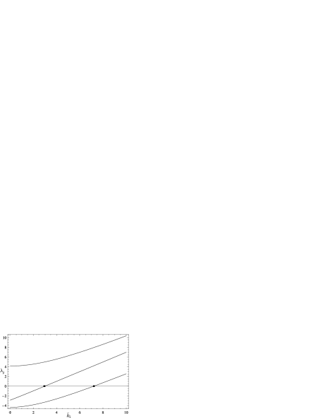
Figure 1: Typical behavior of $B$-matrix eigenvalues, $N=3$. The case of two bound states with energies $E_{1}=-51.8611$ and $E_{2}=-8.8852$ is presented. The black squares show positions of these bound states. The corresponding parameters are $\alpha_{1}=-3$, $\alpha_{2}=-8$, $\alpha_{3}=-1$, $\beta_{12}=0.5$, $\beta_{13}=0.4$, $\beta_{23}=1$, $\Delta_{2}=15$, $\Delta_{3}=25$.

Summarizing, we see that the number of bound states is bounded by $0\leq n_{b}\leq N$. Figure 1 shows the eigenvalues of matrix $B$ as functions of $\bar{k}_{1}$ for the case $N=3$. Two eigenvalues cross the axis which corresponds to the case of $n_{b}=2$. The last comment in this section is devoted to equation (10). Now it can be seen that the factorization energy should be chosen lower than the ground-state energy for the transformed potential, ${\cal E}<E_{g}$, if any.

4 Number of virtual states

According to the definition of a virtual state [1, 2] in this section we will need to consider the channel wave numbers $k_{j}$ lying both in the positive and the negative imaginary semi-axes of the corresponding momenta complex planes and consider the full imaginary axis for $k_{1}$, i.e. $\bar{k}_{1}\in(-\infty,\infty)$. The other momenta, $k_{2},\ldots,k_{N}$, belong to either the positive or to negative parts of their imaginary axes in agreement with the threshold conditions

$$\bar{k}_{j}=\sigma_{j}\sqrt{\bar{k}_{1}^{2}+\Delta_{j}}\,,\qquad\sigma_{j}=\pm\,,\qquad j=2,\ldots,N\,.$$ (26)

Since in (26) all combinations of signs are now possible it is convenient to introduce special notations for these combinations. Denote $\sigma=(+,\pm,\ldots,\pm)$ a string of $N$ signs with $\sigma_{j}$ being its $j$-th entry, which corresponds to the sign in (26) for the $j$-th momentum for $j>1$. The first symbol ”$+$” in $\sigma$ indicates that all momenta $\bar{k}_{j}$ are expressed in terms of $\bar{k}_{1}$. Let $n_{+}(\sigma)+1$ and $n_{-}(\sigma)$ be the numbers of ”$+$” and ”$-$” signs in this string. We notice the following evident combinatoric properties of $n_{-}(\sigma)$ and $n_{+}(\sigma)$. First, $n_{+}(\sigma)+n_{-}(\sigma)+1=N$ which implies

$$\sum\limits_{\sigma}\left[n_{+}(\sigma)+n_{-}(\sigma)+1\right]=N2^{N-1}\,.$$ (27)

Here and in what follows the summation over $\sigma$ includes all $2^{N-1}$ possible sign combinations. Next, a symmetry between ”$+$” and ”$-$” leads to the following relation

$$\sum\limits_{\sigma}n_{-}(\sigma)=\sum\limits_{\sigma}n_{+}(\sigma)=(N-1)2^{N-2}\,.$$ (28)

According to (13) every sign combination leads to its own $B$ matrix defined by the corresponding $K$ matrix so that both $K$ and $B$ should carry an additional information about this combination. Therefore

$$B^{\sigma}=U_{0}+\bar{K}^{\sigma}\,,\qquad\bar{K}^{\sigma}={\rm diag}(\bar{k}_{1},\sigma_{2}\bar{k}_{2},\ldots,\sigma_{N}\bar{k}_{N})$$ (29)

and we denote $\lambda_{j}^{\sigma}(\bar{k}_{1})$, $j=1,\ldots,N$ the eigenvalues of $B^{\sigma}$.

In order to find the zeros of the Jost-matrix determinant corresponding to the virtual states we should find the purely real solutions of the equations $\lambda_{j}^{\sigma}(\bar{k}_{1})=0$, $j=1,\ldots,N$ for all $2^{N-1}$ matrices $B^{\sigma}$. Although the $\bar{k}_{j}$’s are real, but bearing in mind our replacement $k_{j}=i\bar{k}_{j}$, throughout the text we call these zeros purely imaginary. Finally we note that since matrix ${\cal K}-iK$ in (9) is not positive definite for an arbitrary $\sigma$ anymore, in some particular cases some of the zeros of $B$ may be cancelled by the zeros of $\mbox{det}({\cal K}-iK)$ and will not correspond to virtual states. Nevertheless, omitting these particular cases, we will concentrate on an analysis of the zeros of $\mbox{det}B$ only.

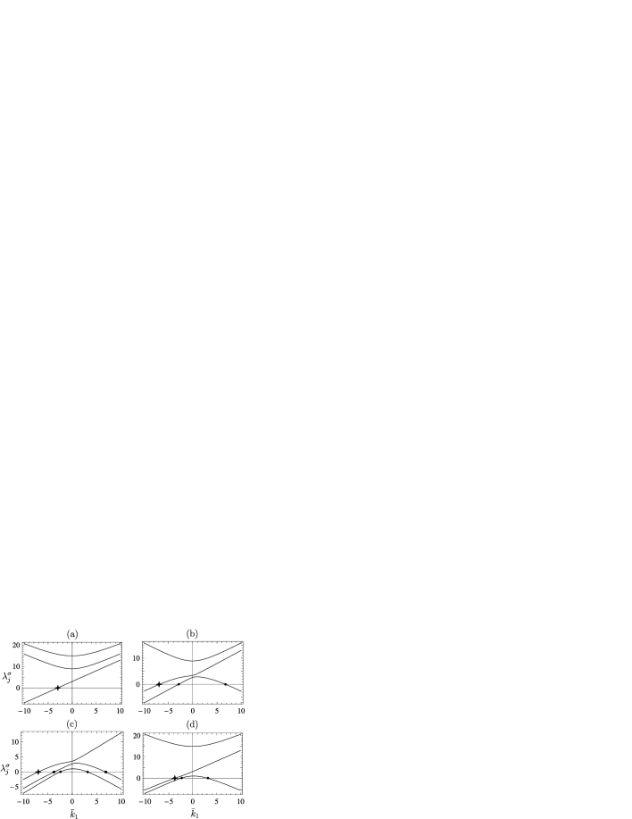
Figure 2: Typical behavior of the eigenvalues $\lambda_{j}^{\sigma}(\bar{k}_{1})$, $N=3$, is shown. Each plane corresponds to a particular choice of string $\sigma$: (a) $\sigma=(+++)$, (b) $\sigma=(++-)$, (c) $\sigma=(+--)$, (d) $\sigma=(+-+)$. Stars, squares and circles correspond to the virtual states. Virtual states are denoted by the identical symbol if they belong to the same eigenvalue $\lambda_{j}^{\sigma}(\bar{k}_{1})$. The corresponding parameters are $\alpha_{1}=3$, $\alpha_{2}=5$, $\alpha_{3}=9$, $\beta_{12}=0.5$, $\beta_{13}=0.4$, $\beta_{23}=0.2$, $\Delta_{2}=15$, $\Delta_{3}=35$.

Eigenvalues $\lambda_{j}^{\sigma}(\bar{k}_{1})$ are monotonous functions of $\bar{k}_{1}$ in two cases only: (i) $\sigma=(+,+,\ldots,+)$ and $\bar{k}_{1}>0$; (ii) $\sigma=(+,-,\ldots,-)$ and $\bar{k}_{1}<0$. In general, an eigenvalue $\lambda_{j}^{\sigma}(\bar{k}_{1})$ may have minima/maxima for $\bar{k}_{1}\lessgtr 0$ which may lead to two or even more roots in equation $\lambda_{j}^{\sigma}(\bar{k}_{1})=0$. We illustrate this behavior for $N=3$ in figure 2. The monotonous lines in the right/left part of figure 2(a)/(c). correspond to case (i)/(ii). The position of the zeros of the eigenvalues is shown by stars, squares and circles. It is clearly seen that the total number of the roots of all equations $\lambda_{j}^{\sigma}(\bar{k}_{1})=0$ is $(N2^{N-1})|_{N=3}=12$ which all correspond to virtual states.

A change of parameters may result in shifting the position of the virtual states only without changing the number of zeros (i.e. virtual states). For instance, in the simplest case we may shift all diagonal entries of $U_{0}$ by a number $\lambda_{0}$, $U_{0}\to U_{0}+\lambda_{0}I$, thus shifting all eigenvalues of $B$ by the same number, ${\lambda}_{j}^{\sigma}(\bar{k}_{1})\to\lambda_{j}^{\sigma}(\bar{k}_{1})+\lambda_{0}$.

Let us consider a specific eigenvalue defined by a string $\sigma_{0}$, with a local maximum at $\bar{k}_{1}=\bar{k}_{1,max}$, $\lambda_{j}^{\sigma_{0}}(\bar{k}_{1,max})=\lambda_{j,max}$. One can always shift all the eigenvalues by the value $\lambda_{j,max}$ such that the curve $\lambda_{j}^{\sigma_{0}}(\bar{k}_{1})$ touches the $\bar{k}_{1}$ axis at the point $\bar{k}_{1}=\bar{k}_{1,max}$ meaning that $\bar{k}_{1,max}$ not only becomes a root of the equation $\lambda_{j}^{\sigma_{0}}(\bar{k}_{1})=0$ but this root is multiple (of multiplicity 2) and by a small additional change of other parameters it can be split into two simple but complex roots. This is just in this way two virtual states collapse producing a resonance; a subject which deserves a special discussion (see the next section). Pairs of virtual states which may collapse are shown in figure 2 by squares and circles.

It is not difficult to convince oneself that for any given $\beta_{jl}$ the situation when all the zeros of the Jost-matrix determinant are purely imaginary may be realized by a proper choice of $\alpha_{j}$. To see that let us consider the asymptotic behavior of $\lambda_{j}^{\sigma}$ for $|\bar{k}_{1}|\rightarrow\infty$, when all off-diagonal entries of $B$ become negligibly small,

$$\lambda_{1}^{\sigma} \simeq \bar{k}_{1}+\alpha_{1}\,,$$ (30)

$$\lambda_{j}^{\sigma} \simeq \sigma_{j}\sqrt{\bar{k}_{1}^{2}+\Delta_{j}}+\alpha_{j}=\sigma_{j}\left(|\bar{k}_{1}|+\frac{\Delta_{j}}{2\bar{k}_{1}}+\ldots\right)+\alpha_{j}\,.$$ (31)

$$|\bar{k}_{1}| \rightarrow \infty\,.$$ (32)

Numbers $n_{+}(\sigma)$ and $n_{-}(\sigma)$ determine the corresponding numbers of increasing and decreasing eigenvalues at positive infinity. The eigenvalue $\lambda_{1}^{\sigma}$ increases both at negative and positive infinity. Now if we choose all $\alpha_{j}$ sufficiently large in absolute values and negative we can always guaranty the location of a root of the equation $\lambda_{1}^{\sigma}(\bar{k}_{1})=0$ near the point $\bar{k}_{1}=\alpha_{1}$ and at the same time the location of two roots of the equation $\lambda_{j}^{\sigma}(\bar{k}_{1})=0$ with corresponding $\sigma_{j}=+$ near the points $\bar{k}_{1}=\pm\alpha_{j}$. Thus, for each $\sigma$ we can obtain $2n_{+}(\sigma)+1$ zeros. The total number $n_{v}$ of these zeros may be calculated by formulas (27) and (28)

$$n_{v}=\sum\limits_{\sigma}[2n_{+}(\sigma)+1]=N2^{N-1}\,,$$ (33)

which coincides with the total number of all possible roots of the system (14), (15) and is just the maximal possible number of virtual states. Hence, in this case all the roots are purely imaginary. In the next section we consider the case when some of the zeros may merge, become complex and produce resonances.

5 Number of resonances

For simplicity independently on whether or not it can be seen in a scattering we call any pair of complex zeros $k=\pm k_{r}+ik_{i}$ of the Jost-matrix determinant a resonance keeping in mind that to be really visible in a scattering a resonance behavior of the corresponding cross-section should be narrow and sharp enough.

Conservation of the number of zeros of an $n$-th order algebraic equation under a variation of parameters included in its coefficients, which keeps unchanged its order (in our case this is equation (19) obtained from the system (14), (15)) applied to our case leads to the following relation $n_{b}+n_{v}+2n_{r}=N2^{N-1}$, where $n_{b}$, $n_{v}$ and $n_{r}$ are number of bound states, virtual states and resonances respectively. The aim of this section is to establish the maximal number of possible resonances accepted by a non-conservative SUSY-partner of the vanishing potential.

Evidently, the maximal number of resonances corresponds to the minimal number of bound $n_{b}$ and virtual $n_{v}$ states. These numbers would both become zero if no one of the $B$ matrix eigenvalues intersected the $\bar{k}_{1}$ axis. But as it was noticed in the previous section there always exists an eigenvalue $\lambda_{1}^{\sigma}$ with the asymptotic behavior given in (30), i.e. ranging from $-\infty$ to $+\infty$ and, hence, it intersects $\bar{k}_{1}$ axis always and for all possible values of $\sigma$. We thus see that the minimal number of real zeros that all eigenvalues may take is achieved if all eigenvalues $\lambda_{j}^{\sigma}(\bar{k}_{1})$, $j>1$ are nodeless and curves $\lambda_{1}^{\sigma}(\bar{k}_{1})$ intersect $\bar{k}_{1}$ axis only once for every given sign combination $\sigma$. To realize this case, we should choose parameters included in $U_{0}$ in a such way that the global minimum $\lambda_{j,min}^{\sigma}$ of every eigenvalue $\lambda_{j}^{\sigma}(\bar{k}_{1})$ with $\sigma_{j}=+$ (they tend to $+\infty$ when $|\bar{k}_{1}|\to\infty$) be positive $\lambda_{j,min}^{\sigma}>0$ and, respectively, global maximum $\lambda_{j,max}^{\sigma}$ of every eigenvalue $\lambda_{j}^{\sigma}(\bar{k}_{1})$ with $\sigma_{j}=-$ (they tend to $-\infty$ when $|\bar{k}_{1}|\to\infty$) be negative $\lambda_{j,max}^{\sigma}<0$. Under these conditions only eigenvalues $\lambda_{1}^{\sigma}(\bar{k}_{1})$ have zeros. The possibility that these eigenvalues have only one zero can always be realized. This can be demonstrated for small enough values of $\beta_{ij}$ (so called weak coupling approximation, see the next section) which in the limit $\beta_{ij}=0$ for all $i,j$ gives a very simple behavior of the eigenvalues. For instance, for $\Delta_{j+1}-\Delta_{j}$ large enough and $\min\limits_{j}(\sqrt{\Delta_{j}}+\alpha_{j})>\max\limits_{j}(-\sqrt{\Delta_{j}}+\alpha_{j})$ the straight line $\lambda_{1}^{\sigma}(\bar{k}_{1})$ never intersects with the hyperbolas $\lambda_{j}^{\sigma}(\bar{k}_{1})$ so that small perturbations coming from small non-zero $\beta_{jl}$-values (in a physical terminology these perturbations shift the zero width resonances from the real energy axis to the complex plane) do not change the monotonous behavior of $\lambda_{1}^{\sigma}(\bar{k}_{1})$ and, hence, do not bring additional roots to the equation $\lambda_{1}^{\sigma}(\bar{k}_{1})=0$.

Thus, we see that the minimal value of virtual states with the absence of bound states is equal to all possible sign combinations of $\sigma$ which is $n_{vmin}=\sum\limits_{\sigma}1=2^{N-1}$. Hence, the maximal possible number of resonances is obtained by subtracting this number from the total number of solutions, i.e.

$$2n_{r,max}=N2^{N-1}-2^{N-1}=(N-1)2^{N-1}\,.$$ (34)

6 Weak coupling approximation

For the number of channels $N>2$ there is no way to get analytical solutions of system (14), (15) but if the coupling parameters $\beta_{ij}$ are small enough assuming analyticity of the roots of the Jost-matrix determinant as functions of $\beta_{ij}$ a perturbation technique may be developed. In this section we demonstrate this possibility by obtaining first order corrections to unperturbed values of the roots of the Jost-matrix determinant corresponding to $\beta_{ij}=0$.

For the zero coupling, matrix $U_{0}$ becomes diagonal $U_{0}=\mbox{diag}(\alpha_{1},\alpha_{2},\ldots,\alpha_{N})$ and the system (11), (3) reduces to

$$(\alpha_{1}-ik_{0,1})(\alpha_{2}-ik_{0,2})\ldots(\alpha_{N}-ik_{0,N})=0\,,$$ (35)

$$k_{0,j}^{2}-k_{0,1}^{2}+\Delta_{j}=0\,,\qquad j=2,\ldots,N\,,$$ (36)

where the additional subscript $0$ corresponds to the uncoupled case. Its solutions have the form

$$k_{0,1}^{(1,\sigma)} = -i\alpha_{1}\,,\quad k_{0,m}^{(1,\sigma)}=\sigma_{m}\sqrt{-\alpha_{1}^{2}-\Delta_{m}}\,,\quad m\neq 1\,,$$

$$k_{0,2}^{(2,\sigma)} = -i\alpha_{2}\,,\quad k_{0,m}^{(2,\sigma)}=\sigma_{m}\sqrt{-\alpha_{2}^{2}+\Delta_{2}-\Delta_{m}}\,,\quad m\neq 2\,,$$

$$\ldots$$

$$k_{0,N}^{(N,\sigma)} = -i\alpha_{N}\,,\quad k_{0,m}^{(N,\sigma)}=\sigma_{m}\sqrt{-\alpha_{N}^{2}+\Delta_{N}-\Delta_{m}}\,,\quad m\neq N\,,$$ (37)

where $m=1,\ldots,N$. Let us explicitly indicate the meaning of sub- and superscripts in (37): the second subscript $m$ in $k_{0,m}^{(j,\sigma)}$ corresponds to the channel, the first superscript $j$ indicates a row number in (37) and $\sigma$ indicates one of all $2^{N-1}$ combinations of signs. Thus, we see once again that the total number of solutions of the system is $N2^{N-1}$ and it does not depend on whether or not the coupling is absent. Note that every energy level $E_{j}=-\alpha_{j}^{2}+\Delta_{j}$ corresponding to a row in (37) is $2^{N-1}$ fold degenerate. Below we show that under a small coupling every degenerate level $E_{j}$ splits by $2^{N-1}$ sub-levels and we will find approximate values of the splitting. But the unperturbed $j$-th momentum corresponding to this level simply equals $k_{0,j}^{(j,\sigma)}=-i\alpha_{j}$. Therefore, instead of our previous convention to express all quantities in terms of $k_{1}$, it is convenient here to express corrections to the $j$-th momentum produced by a perturbation in terms of unperturbed $j$-th momentum $\bar{k}_{0,j}^{(j,\sigma)}$. This is always possible due to the fact that all momenta have equal rights. But now we have to change our signs convention introduced in section 4 where the first momentum $\bar{k}_{1}$ entered in the string $\sigma$ always with the positive sign ($\sigma_{1}=+$). Now we have $j$-th momentum $\bar{k}_{j}\in(-\infty,\infty)$ and $\sigma_{j}=+$ in string $\sigma$.

From (37) we learn that no coupling implies no finite-width resonances but as we discuss below the zeros lying above the first threshold may be associated with zero-width resonances which acquire a non-zero width under a small coupling.

From the first row of (37) we conclude that the corresponding $2^{N-1}$ zeros with $E_{1}=-\alpha_{1}^{2}$ are always below the first threshold (bound or virtual states). Energy $E_{n}=-\alpha_{n}^{2}+\Delta_{n}$, $n=2,\ldots,N$, may be positive with respect to the first threshold and just these $(N-1)2^{N-1}$ zeros are associated with the zero-width resonances. According to our convention a resonance corresponds to a pair of complex zeros. Here we can easily compute the number of the zero-width resonances, $n_{zwr}$, which is $n_{zwr}=(N-1)2^{N-2}$ which agrees with the maximal number of possible resonances obtained in the previous section.

Unperturbed $B^{\sigma}$ matrix we denote $B^{\sigma}_{0}$ is diagonal

$$B_{0}^{\sigma}={\rm diag}(\alpha_{1}+\sigma_{1}\bar{k}_{1},\alpha_{2}+\sigma_{2}\bar{k}_{2},\ldots,\alpha_{N}+\sigma_{N}\bar{k}_{N})$$ (38)

and its eigenvalues $\lambda_{0,j}^{\sigma}$ coincide with its diagonal entries

$$\lambda_{0,j}^{\sigma}(\bar{k}_{j})=\alpha_{j}+\bar{k}_{j}\,,\qquad\lambda_{0,l}^{\sigma}(\bar{k}_{j})=\alpha_{l}+\sigma_{l}\sqrt{\bar{k}_{j}^{2}+\Delta_{l}-\Delta_{j}}\,,$$ (39)

$$l=1,\ldots,N\,,\qquad l\neq j\,.$$ (40)

For simplicity we assume all coupling parameters $\beta_{ij}$ proportional to the same small parameter $\beta$ so that the perturbed $B^{\sigma}$ matrix reads

$$B^{\sigma}=B_{0}^{\sigma}+\beta\mathcal{B}\,,\quad\mathcal{B}=||b_{jl}||\,,\quad b_{jj}=0\,,\quad j=1,\ldots,N\,.$$ (41)

Now as it was mentioned above assuming analyticity of eigenvalues of this matrix as functions of $\beta$ we can develop them in a Taylor series with respect to $\beta$,

$$\tilde{\lambda}_{j}^{\sigma}=\lambda_{0,j}^{\sigma}+\lambda_{1,j}^{\sigma}+\lambda_{2,j}^{\sigma}+\ldots\,,$$ (42)

where the first subscript number is just the power of $\beta$. First we notice that the perturbation $\mathcal{B}$ has zero diagonal entries which results in $\lambda^{\sigma}_{1,j}=0$. To get the second order correction we are using the usual Rayleigh-Schrödinger perturbation approach which leads to

$$\lambda_{2,j}^{\sigma}(\bar{k}_{j})=\beta^{2}\sum\limits_{l=1,\,l\neq j}^{N}\frac{b_{jl}^{2}}{\lambda_{0,j}^{\sigma}(\bar{k}_{j})-\lambda_{0,l}^{\sigma}(\bar{k}_{j})}\,.$$ (43)

In what follows we also assume that we can neglect the higher-order corrections to the eigenvalues.

Actually, our aim is to find corrections to the unperturbed degenerate $j$-th Jost-matrix determinant zero given in (37). Assuming a Taylor series expansions for this root over the small parameter $\beta$ indicating it now explicitly

$$\bar{k}_{j}=\bar{k}_{0,j}^{(j,\sigma)}+\beta c_{1}+\beta^{2}c_{2}+\ldots$$ (44)

we find coefficients $c_{1}$ and $c_{2}$ from the equation

$$\tilde{\lambda}_{j}^{\sigma}(\bar{k}_{j})=\lambda^{\sigma}_{0,j}(\bar{k}_{j})+\lambda^{\sigma}_{2,j}(\bar{k}_{j})=0\,.$$ (45)

For that we develop $\tilde{\lambda}_{j}^{\sigma}(\bar{k}_{j})$ in a Taylor series in $\beta$ parameter considering its $\beta$ dependence as given through $\bar{k}_{j}$ and (44). The term (43) contains the factor $\beta^{2}$, therefore in its denominator we simply put $\bar{k}_{0,j}^{j,\sigma}$ instead of $\bar{k}_{j}$. The $\bar{k}_{j}$-dependence of the term $\lambda^{\sigma}_{0,j}(\bar{k}_{j})$ is given by (39) and its $\beta$-dependence is obtained via (44). Thus, the left hand side of equation (45) is presented as a series over the powers of $\beta$ where every coefficient should vanish. This leads to $c_{1}=0$ and

$$c_{2}=\sum\limits_{l=1,\,l\neq j}^{N}\frac{b_{jl}^{2}}{\alpha_{l}+\sigma_{l}\sqrt{\alpha_{j}^{2}+\Delta_{l}-\Delta_{j}}}\,.$$ (46)

Finally up to the second order in $\beta$ we obtain the roots of system (37)

$$\begin{array}[]{lll}k_{1}^{(1,\sigma)}&=&-i\alpha_{1}+i\sum\limits_{l=2}^{N}\frac{\beta^{2}b_{1l}^{2}}{\alpha_{l}+\sigma_{l}\sqrt{\alpha_{1}^{2}+\Delta_{l}}}\,,\quad k_{m}^{(1,\sigma)}=\sigma_{m}\sqrt{\left(k_{1}^{(1,\sigma)}\right)^{2}-\Delta_{m}}\,,\\ k_{2}^{(2,\sigma)}&=&-i\alpha_{2}+i\sum\limits_{l=1,\,l\neq 2}^{N}\frac{\beta^{2}b_{2l}^{2}}{\alpha_{l}+\sigma_{l}\sqrt{\alpha_{2}^{2}+\Delta_{l}-\Delta_{2}}}\,,\quad k_{m}^{(2,\sigma)}=\sigma_{m}\sqrt{\left(k_{2}^{(2,\sigma)}\right)^{2}+\Delta_{2}-\Delta_{m}}\,,\\ &\ldots&\\ k_{N}^{(N,\sigma)}&=&-i\alpha_{N}+i\sum\limits_{l=1}^{N-1}\frac{\beta^{2}b_{Nl}^{2}}{\alpha_{l}+\sigma_{l}\sqrt{\alpha_{N}^{2}+\Delta_{l}-\Delta_{N}}}\,,\quad k_{m}^{(N,\sigma)}=\sigma_{m}\sqrt{\left(k_{N}^{(N,\sigma)}\right)^{2}+\Delta_{N}-\Delta_{m}}\,.\end{array}$$

Here each row is obtained by applying equations (43), (44), (45) and (46) for $j=1,\ldots,N$, respectively, and $m=1,\ldots,N$, $m\neq j$ for each $j$. The square roots in the last column of (6) should be expanded in Taylor series up to $\beta^{2}$.

From here it is easily seen that, when $\alpha_{m}^{2}<\Delta_{m}$, purely imaginary unperturbed zeros $k_{m}=-i\alpha_{m}$ move from the axes to the complex plane due to the real part of corrections. For instance for $k_{2}$, the real part reads ${\pm\beta^{2}\sqrt{\Delta_{2}-\alpha_{2}^{2}}/(\alpha_{1}^{2}-\alpha_{2}^{2}+\Delta_{2})}$. We thus confirmed the previous statement that zero width resonances acquire non-zero widths.

7 Zeros of the Jost-matrix determinant for $N=2$

The particular case of two coupled channels is important both from practical and theoretical point of view. Let us recall the following inequalities for the number of the bound/virtual states and resonances obtained in sections 3, 4 and 5: $0\leq n_{b}\leq 2$, $0\leq n_{r}\leq 1$, $0\leq n_{v}\leq 4$. The same inequalities are obtained for $N=2$ in [10, 11] from another approach. The two-channel problem is the only one where one is able to get analytic expressions for the Jost-determinant roots, i.e. to solve the direct problem consisting in finding the positions of the bound/virtual states and resonances. This possibility is based on the fact that the roots of the algebraic equation of fourth, $(N2^{N-1})|_{N=2}=4$, order may be expressed in radicals. Thus we obtain zeros as functions of parameters defining the potential. One may be interested in solving the inverse problem: to express parameters of the potential from the knowledge about positions of zeros of the Jost-matrix determinant. In principle, one may try to inverse radicals, but we propose a more elegant way below.

To simplify the notations, we choose in this case $\Delta_{2}\equiv\Delta\neq 0$. The potential, which is known as the Cox potential [8], depends on three parameters appearing in matrix

$$U_{0}=\left(\begin{array}[]{cc}\alpha_{1}&\beta\\ \beta&\alpha_{2}\end{array}\right)$$ (47)

and on the factorization energy $\cal E$ which is upper bounded. The Jost-matrix determinant reads

$$f(k_{1},k_{2})\equiv\mbox{det}F(k_{1},k_{2})=\frac{(k_{1}+i\alpha_{1})(k_{2}+ia_{2})+\beta^{2}}{({k_{1}+i\kappa_{1}})(k_{2}+i\kappa_{2})}.$$ (48)

The system of equations (14), (15) in this case takes the simplest form

$$k_{1}^{2}-k_{2}^{2}=\Delta,$$ (49)

$$(k_{1}+i\alpha_{1})(k_{2}+i\alpha_{2})+\beta^{2}=0$$ (50)

and can be reduced to a fourth order algebraic equation with respect to $k_{1}$

$$k_{1}^{4}+ia_{1}k_{1}^{3}+a_{2}k_{1}^{2}+ia_{3}k_{1}+a_{4}=0\,.$$ (51)

The coefficients $a_{i}$, $i=1,\ldots,4$ are given explicitly in [10], (33a-d). Momentum $k_{2}$ can be found from

$$k_{2}(ik_{1}-\alpha_{1})=\alpha_{2}(k_{1}+i\alpha_{1})-i\beta^{2}\,,$$ (52)

which is a direct implication of (50). Equations (51) and (52) are particular case of the system (19), (18), …, (16) for $N=2$ in accordance with our general discussion in section 2.

Let us assume we have found two of the roots of system (49), (50) we denote $(k_{1}^{(1)},k_{2}^{(1)})$ and $(k_{1}^{(2)},k_{2}^{(2)})$, which clearly are functions of parameters $\alpha_{1}$ and $\alpha_{2}$. Their dependence on parameters $\beta$ and $\Delta$ is not important for the moment, since both $\beta$ and $\Delta$ assumed to be fixed. Being put back to (50) the equation reduces twice to identity for any values of $\alpha_{1}$ and $\alpha_{2}$, which we write as

$$(k_{1}^{(1)}+i\alpha_{1})(k_{2}^{(1)}+i\alpha_{2})+\beta^{2}=0\,,$$ (53)

$$(k_{1}^{(2)}+i\alpha_{1})(k_{2}^{(2)}+i\alpha_{2})+\beta^{2}=0\,.$$ (54)

The reason why we replaced the identity sign by the equality sign is that these equations may be considered as an implicitly written inverted dependence of $\alpha_{1,2}$ on the set of parameters $k_{1,2}^{(1,2)}$. We may thus fix arbitrary values for $k_{1,2}^{(1,2)}$ and find from (53), (54) $\alpha_{1}$ and $\alpha_{2}$ in terms of $k_{1,2}^{(1,2)}$ which is a much easier task than finding an explicit dependence of $k_{1,2}^{(1,2)}$ on $\alpha_{1}$ and $\alpha_{2}$. For that we have to solve, e.g. for $\alpha_{1}$, the following second order equation

$$\alpha_{1}^{2}-\alpha_{1}i(k_{1}^{(1)}+k_{1}^{(2)})-k_{1}^{(1)}k_{1}^{(2)}+\beta^{2}\frac{R_{1}}{R_{2}}=0\,,$$ (55)

with $R_{1}=k_{1}^{(2)}-k_{1}^{(1)}$ and $R_{2}=k_{2}^{(2)}-k_{2}^{(1)}$ which easily follows from (53) and (54). From here we find

$$\alpha_{1} = \frac{1}{2}\left[i(k_{1}^{(1)}+k_{1}^{(2)})\pm\sqrt{-R_{1}^{2}-4\beta^{2}R_{1}/R_{2}}\right],$$ (56)

$$\alpha_{2} = \frac{1}{2}\left[i(k_{2}^{(1)}+k_{2}^{(2)})\mp\sqrt{-R_{2}^{2}-4\beta^{2}R_{2}/R_{1}}\right].$$ (57)

The upper (resp., lower) sign in (57) corresponds to the upper (resp., lower) sign in (56). The values of $k_{1}^{(1,2)}$ and $k_{2}^{(1,2)}$ should be chosen so as to warranty the reality of parameters $\alpha_{1,2}$.

Once two roots are fixed, (51) reduces to a second-order algebraic equation $\mathcal{Q}_{2}(k_{1})=0$ for the two other roots $k_{1}^{(3)}$ and $k_{1}^{(4)}$ thus providing an implicit but rather simple mapping between the roots of system (49), (50) and the set of parameters $(\alpha_{1},\alpha_{2},\beta)$. Polynomial $\mathcal{Q}_{2}(k_{1})$ is the ratio of the polynomial appearing in (51) and ${\mathcal{P}_{2}(k_{1})=k_{1}^{2}-k_{1}(k_{1}^{(2)}+k_{1}^{(1)})+k_{1}^{(2)}k_{1}^{(1)}}$, i.e.,

$$k_{1}^{4}+ia_{1}k_{1}^{3}+a_{2}k_{1}^{2}+ia_{3}k_{1}+a_{4}=\mathcal{P}_{2}(k_{1})\mathcal{Q}_{2}(k_{1})\,.$$

From here we find, with the explicit expression for coefficients $a_{i}$, $i=1,\ldots,4$ [10],

$$\mathcal{Q}_{2}(k_{1})=(k_{1}+i\alpha_{1})^{2}+k_{1}(k_{1}^{(2)}+k_{1}^{(1)})+$$

$$(2i\alpha_{1}+k_{1}^{(2)}+k_{1}^{(1)})(k_{1}^{(2)}+k_{1}^{(1)})+\alpha_{2}^{2}-\Delta-k_{1}^{(1)}k_{1}^{(2)}$$

and, hence,

$$k_{1}^{(3)}=\frac{1}{2}\left[\mp i\sqrt{-R_{1}^{2}-4\beta^{2}R_{1}/R_{2}}+\sqrt{D_{1}}\right],$$ (58)

$$k_{1}^{(4)}=\frac{1}{2}\left[\mp i\sqrt{-R_{1}^{2}-4\beta^{2}R_{1}/R_{2}}-\sqrt{D_{1}}\right],$$ (59)

where $D_{1}=R_{1}^{2}+4\beta^{2}\frac{R_{2}}{R_{1}}+4k_{1}^{(2)}k_{1}^{(1)}$. The sign before the first square root in (58) and (59) should be chosen in accordance with the signs in (56) and (57).

To find $k_{2}^{(3,4)}$ we do not need to solve any equation. We simply notice that the equation $\mbox{det}F(k_{1},k_{2})=0$ is invariant under the transformation $k_{1}\leftrightarrow k_{2}$, $\alpha_{1}\leftrightarrow\alpha_{2}$, $\Delta\leftrightarrow-\Delta$. This means that being transformed according to these rules equations (58) and (59) give us the $k_{2}$ values:

$$k_{2}^{(3)}=\frac{1}{2}\left[\mp i\sqrt{-R_{2}^{2}-4\beta^{2}R_{2}/R_{1}}-\sqrt{D_{2}}\right],$$ (60)

$$k_{2}^{(4)}=\frac{1}{2}\left[\mp i\sqrt{-R_{2}^{2}-4\beta^{2}R_{2}/R_{1}}+\sqrt{D_{2}}\right],$$ (61)

where $D_{2}=R_{2}^{2}+4\beta^{2}\frac{R_{1}}{R_{2}}+4k_{2}^{(2)}k_{2}^{(1)}$.

Table 1: Possible mappings between some experimental data and the Cox potential parameters.

Experimental	Fixed	Free	Restrictions
data	parameters	parameters
$\Delta\,,E_{r}\,,E_{i}$	$\alpha_{1}\,,\alpha_{2}\,$	$\kappa_{1},\beta$	$\beta\geq\sqrt{-k_{r}p_{r}}$
$\Delta\,,E_{b}=-\lambda_{b}^{2}\,,E_{r}\,,E_{i}$	$\alpha_{1}\,,\alpha_{2}\,,\beta$	$\kappa_{1}$	$\kappa_{1}>\lambda_{b}$
$\Delta\,,E_{1,2}=-\lambda_{1,2}^{2}$	$\alpha_{1}\,,\alpha_{2}\,$	$\kappa_{1},\beta$	$\kappa_{1}>\lambda_{2}>\lambda_{1}$
$\Delta\,,E_{b}=-\lambda_{b}^{2}$	$\alpha_{2}\,$	$\kappa_{1}\,,\beta\,,\alpha_{1}$	$\kappa_{1}>\lambda_{b}$

Two initial zeros $(k_{1}^{(1)},k_{2}^{(1)})$, $(k_{1}^{(2)},k_{2}^{(2)})$ and threshold difference $\Delta$ are assumed to be known from the experiment. For instance, these zeros may correspond to a visible Feshbach resonance or two bound states. The possible cases for initial data are summarized in Table 1. The first row of Table 1 corresponds to the case where the position of the resonance is known (see section 7.1 below). The second row corresponds to the case where the positions of both the resonance and one bound state are known, which allows one to fix maximal number of parameters. The third row corresponds to the case where the positions of two bound states are known (see section 7.2 below). The last row corresponds to the special case when only one zero may be fixed from experimental data. The free parameters in Table 1 allow either for isospectral deformations of the potential or for fits of additional experimental data as, e.g., scattering lengths (see e.g. [10, 11]). The restriction on the factorization energy is deduced from the regularity condition of the potential (10). The restriction on the coupling parameter $\beta$ is explained below (see (66) in section 7.1). Let us now consider examples corresponding to the first three rows of Table 1.

7.1 One resonance.

A resonance corresponds to a pair of complex roots $k_{1}^{(1)}$ and $k_{1}^{(2)}$ of the Jost-matrix determinant such that $ik_{1}^{(1)}$ and $ik_{1}^{(2)}$ are mutually complex conjugate. Therefore we assume equations (49) and (50) to have two complex roots. Let us define their first-channel components as

$$k_{1}^{(1)}=k_{r}+ik_{i}\,,\quad k_{1}^{(2)}=-k_{r}+ik_{i}\,,\quad k_{i}\in\mathbb{R}\,,\quad k_{r}\in\mathbb{R}\,,\quad k_{r}>0\,,$$ (62)

and write the corresponding energies, $\left(k_{1}^{(1,2)}\right)^{2}$, as $E_{r}\pm iE_{i}$, where we also assume $E_{i}>0$ (which means that the upper sign corresponds to $k_{1}^{(1)}$ or $k_{1}^{(2)}$, depending on the sign of $k_{i}$). We would like to choose as parameters the threshold difference $\Delta$, as well as the real and imaginary parts of the resonance complex energy, $E_{r},E_{i}$. As exemplified below, these can correspond to physical parameters of a visible resonance in some (but not all) cases. In terms of these parameters, $k_{r}$ and $k_{i}$ are expressed as

$$k_{r}=\frac{E_{i}}{\sqrt{2}}\,\left[\sqrt{E_{r}^{2}+E_{i}^{2}}-E_{r}\right]^{-1/2},\quad k_{i}=\pm\frac{1}{\sqrt{2}}\,\left[\sqrt{E_{r}^{2}+E_{i}^{2}}-E_{r}\right]^{1/2}.$$ (63)

In the second channel the roots

$$k_{2}^{(1)}=p_{r}+ip_{i}\,,\quad k_{2}^{(2)}=-p_{r}+ip_{i}\,,$$

can be found from the threshold condition yielding

$$p_{r} = -\frac{1}{\sqrt{2}}\,\left[\sqrt{E_{i}^{2}+(E_{r}-\Delta)^{2}}+E_{r}-\Delta\right]^{1/2}\!\!,$$ (64)

$$p_{i} = \mp\frac{E_{i}}{\sqrt{2}}\,\left[\sqrt{E_{i}^{2}+(E_{r}-\Delta)^{2}}+E_{r}-\Delta\right]^{-1/2}\!\!\!\!\!\!.$$ (65)

The upper (resp., lower) sign in (63) corresponds to the upper (resp., lower) sign in (65), which means that, for a given zero, the signs of $k_{i}$ and $p_{i}$ are opposite. Moreover, equations (63) and (64) show that, for a given zero, the signs of $k_{r}$ and $p_{r}$ are also opposite. This implies that, for the Cox potential, the complex resonance zeros (or scattering-matrix poles) are always in opposite quadrants in the complex $k_{1}$ and $k_{2}$ planes.

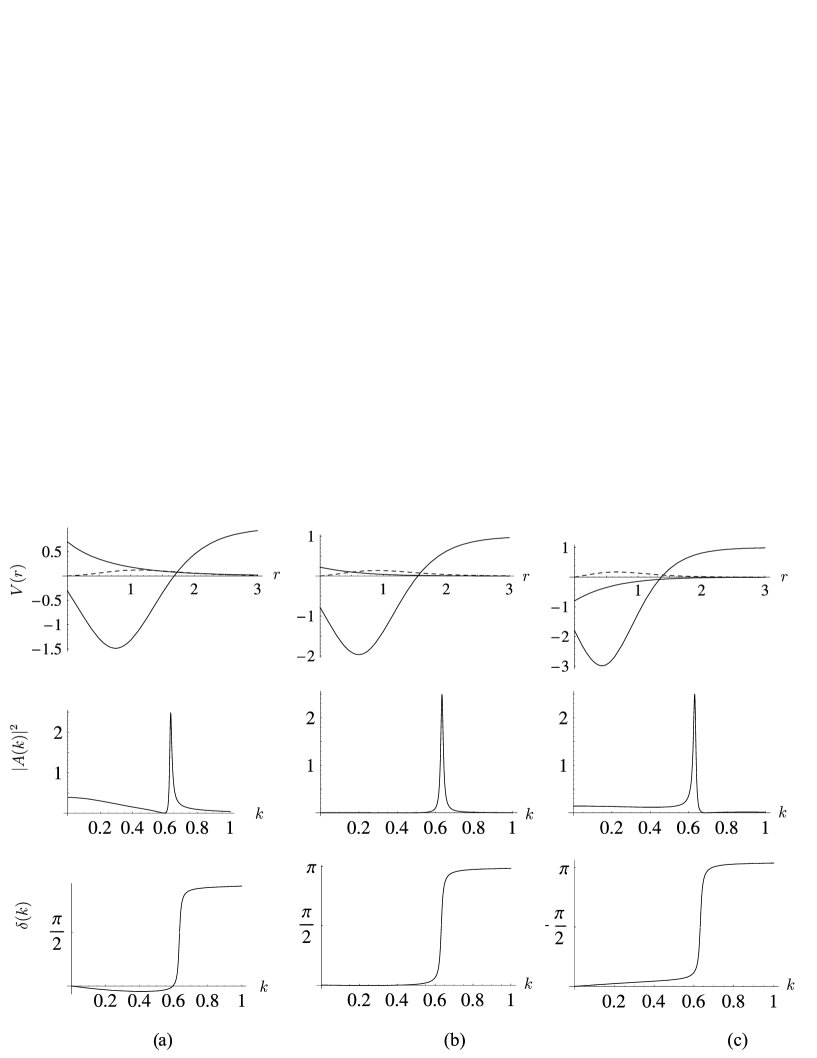
Figure 3: The Cox potential without bound state and with one visible resonance of energy $E_{r}=0.4$ and width $\Gamma=0.02$, for $\Delta=1$ and $\beta=0.1$ (first row, solid lines for $V_{11}$ and $V_{22}+\Delta$, dashed line for $V_{12}$), with the corresponding partial cross section (second row) and phase shifts (third row) for (a) $\kappa_{1}=0.5$; (b) $\kappa_{1}=0.7$; (c) $\kappa_{1}=1$.

This has important consequences for physical applications: for a resonance to be visible, one of the corresponding zero has to lie close to the physical positive-energy region, i.e., close to the real positive $k_{1}$ axis and close to the region made of the real positive $k_{2}$ axis and of the positive imaginary $k_{2}$ interval: $[0,i\sqrt{\Delta}]$. Consequently, the only possibility for a visible resonance with the Cox potential is that of a Feshbach resonance, only visible in the channel with lowest threshold, with an energy lying below threshold $\Delta$. At higher resonance energies, the corresponding zero is either close to the $k_{1}$-plane physical region (and far from the $k_{2}$-plane one) or close to the $k_{2}$-plane physical region (and far from the $k_{1}$-plane one); it cannot be close to both physical regions at the same time, hence it cannot have a visible impact on the coupled scattering matrix. Here, we illustrate the case of a visible resonance, which is the most interesting from the physical point of view. It corresponds to the lower signs in (63) and (65), with a resonance energy $E_{r}$ such that $0<E_{r}<\Delta$, and a resonance width $\Gamma=2E_{i}$ such that $E_{i}<E_{r}$.

Note, that for non-zero values of the parameters $k_{r}$ and $p_{r}$ (which have opposite signs), the coupling parameter $\beta$ cannot be infinitesimal: because $\alpha_{1}$ and $\alpha_{2}$ have to be real, $\beta$ is restricted to satisfy the inequality

$$\beta\geq\sqrt{-k_{r}p_{r}}\,.$$ (66)

To get a potential with one bound state at energy $-\lambda_{b}^{2}$, we choose the lower signs in (56), (57). We then get for $k_{1}^{(3)}(\beta)$ an expression similar to (58), (59), from which the value of $\beta$ can be found by solving the bi-squared equation $k_{1}^{(3)}(\beta)=i\lambda_{b}$.

Let us now choose explicit parameters. First, we put $\Delta=1$. To get a visible resonance, we put $E_{r}=0.4$, $E_{i}=0.01$ (which corresponds to a resonance width $\Gamma=0.02$), and $\beta=0.1$. Using (56), (62) and (63), one finds $\alpha_{1}=0.76938$ and $\alpha_{2}=-0.766853$ (we choose the upper signs (56), (57)). The factorization energy, $\cal E$, is not constrained in this case: it just has to be negative. The Cox potential with one resonance and two virtual states $E_{v1}=-0.560473$, $E_{v2}=-0.599544$ is shown in the first row of figure 3.

The diagonal elements of the potentials, $V_{11}$ and $V_{22}+\Delta$, are plotted with solid lines, while $V_{12}$ is plotted with dashed lines. Parameter $\kappa_{1}$ is responsible for the isospectral deformation of the potential which results in the behavior of the phase shifts. The second row of figure 3 shows the corresponding partial cross sections, where the resonance behavior is clearly seen, as well as the evolution of the low-energy cross section, which is related to the scattering length. The last row of figure 3 shows the corresponding phase shifts for the open channel, where a typical Breit-Wigner behavior (see e.g. Ref. [1]) is seen for the resonance, as well as the evolution of the zero-energy phase-shift slope, which is also related to the scattering length.

7.2 Two bound states

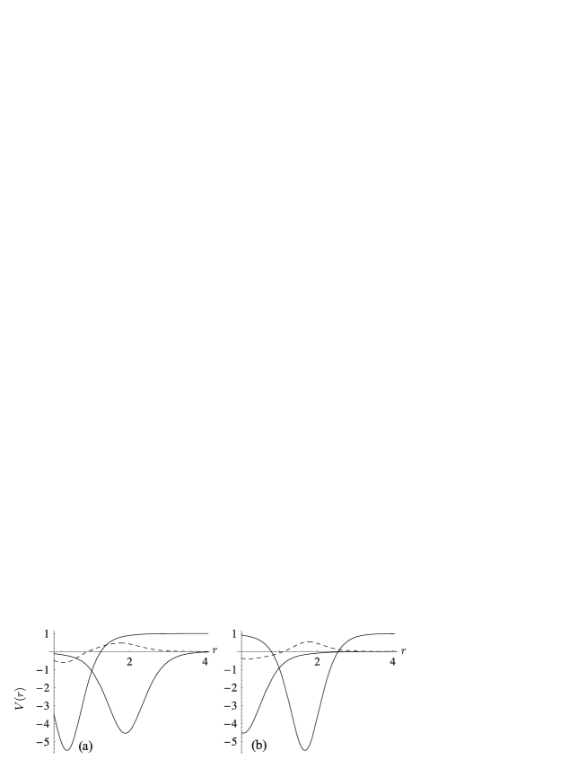
Figure 4: The Cox potential (solid lines for $V_{11}$ and $V_{22}+\Delta$, dashed line for $V_{12}$) with two bound states at energies $E_{1}=-0.01$ and $E_{2}=-2.25$, for $\Delta=1$, $\beta=0.1$ and $\kappa_{1}=1.51$. The left (resp., right) graphic corresponds to the upper (resp., lower) signs in (56) and (57).

Let us now construct a Cox potential with two bound states, and hence no resonance [10]. We choose $k_{1}^{(1)}=0.1i$ and $k_{1}^{(2)}=1.5i$ for these bound states and, as in the previous example, we put $\Delta=1$ and $\beta=0.1$. We thus have $k_{2}^{(1)}=\sqrt{1.01}i$ and $k_{2}^{(2)}=\sqrt{3.25}i$, which defines $R_{2}$ in (56), (57). Choosing the upper signs in these equations, we find $\alpha_{1}=-0.112649$ and $\alpha_{2}=-1.79557$, while for the lower signs, we get $\alpha_{1}=-1.48735$ and $\alpha_{2}=-1.0122$. The corresponding Cox potentials are shown in figure 4.

8 Conclusion

A careful study of spectral properties of non-conservative multichannel SUSY partners of the zero potential is given. Our treatment is based on the analysis of the Jost-matrix determinant zeros. Generalizing our previous results for the two-channel case [10, 11], we have shown that the zeros of the Jost-matrix determinant are the roots of an $N2^{N-1}$th-order algebraic equation. The number of bound states $n_{b}$ is restricted by the number of channels, $0\leq n_{b}\leq N$. The upper bound for the number of resonances is $(N-1)2^{N-2}$. The generalization is based on the analysis of the behavior of the Jost-matrix eigenvalues.

In general, an algebraic equation of an order higher than $4$ has no solutions in radicals. As a consequence, there are no exact analytic solutions of a spectral problem for a non-conservatively SUSY transformed Hamiltonian with $N>2$. Therefore, the problem of finding the approximate solutions appears to be actual. Based on the usual Rayleigh-Schrödinger perturbation theory for the eigenvalues of the Jost matrix we develop an approximate method for finding the zeros of the Jost-matrix determinant in the case of a weak coupling between channels.

An analytical study of the Jost-determinant zeros is carried out for the two-channel case which implies an algebraic equation of the fourth order. A suitable factorization of the fourth-order polynomial allows us to develop a procedure which solves the inverse spectral problem for this case. The effectiveness of the procedure is illustrated by two examples: a potential with one resonance and a potential with two bound states.

References

References

- [1] Taylor J R 1972 Scattering Theory: The Quantum Theory on Nonrelativistic Collisions (New York: Wiley)
- [2] Newton R G 2002 Scattering Theory of Waves and Particles (New York: Dover)
- [3] Sukumar C V 1985 Supersymmetric quantum mechanics and the inverse scattering method J. Phys. A: Math. Gen. 18 2937-55
- [4] Sparenberg J-M, Samsonov B F, Foucart F and Baye D 2006 Multichannel coupling with supersymmetric quantum mechanics and exactly-solvable model for Feshbach resonance J. Phys. A: Math. Gen. 39 L639-45 (Preprint quant-ph/0601101v2)
- [5] Samsonov B F, Sparenberg J-M and Baye D 2007 Supersymmetric transformations for coupled channels with threshold differences J. Phys. A: Math. Theor. 40 4225-40 (Preprint math-ph/0612029)
- [6] Amado R D, Cannata F and Dedonder J-P 1988 Coupled-channel supersymmetric quantum mechanics Phys. Rev. A 38 3797-800
- [7] Amado R D, Cannata F and Dedonder J-P 1988 Formal scattering theory approach to S-matrix relations in supersymmetric quantum mechanics Phys. Rev. Lett. 61 2901
- [8] Cox J R 1964 Many-channel Bargmann potentials J. Math. Phys. 5 1065-9
- [9] Vidal F and LeTourneux J 1992 Multichannel scattering with nonlocal and confining potentials. II. Application to a nonrelativistic quark model of the NN interaction Phys. Rev. C 45 430-6
- [10] Pupasov A M, Samsonov B F and Sparenberg J-M 2007 Exactly-solvable coupled-channel potential models of atom-atom magnetic Feshbach resonances from supersymmetric quantum mechanics (Preprint quant-ph/0709.0343)
- [11] Pupasov A M, Samsonov B F and Sparenberg J-M 2008 Exactly-solvable coupled-channel potential models of atom-atom magnetic Feshbach resonances from supersymmetric quantum mechanics Phys. Rev. A 77 012724-14