THE SPATIAL DISTRIBUTION FUNCTION OF GALAXIES AT HIGH REDSHIFT

Abstract

This is the first exploration of the galaxy distribution function at redshifts greater than about 0.1. Redshifts are based on the North and South GOODS Catalogs. In each catalog we examine clustering in the two redshift bands $0.47\leq z\leq 0.8$ and $0.9\leq z\leq 1.5$. The mean redshifts of the samples in these bands are about $0.6$ and $1.1$. Our main result is that at these redshifts the galaxy spatial distribution function $f_{V}(N)$ has the form predicted by gravitational quasi-equilibrium dynamics for cosmological many-body systems. This constrains related processes such as galaxy merging and the role of dark matter in the range of these redshifts.

1. Introduction

At relatively low redshifts, $z\lesssim 0.1$, several surveys have determined the distribution function of galaxies and their associated dark matter. These include the Zwicky Catalog (Crane & Saslaw, 1986) the UGC and ESO Catalogs (Lahav & Saslaw, 1992), the SSRS Catalog in three dimensions (Fang & Zou, 1994), the Pisces-Persus Supercluster (Saslaw & Haque-Copilah, 1998) and most recently the 2MASS Catalog with about 650,000 galaxies (Sivakoff & Saslaw, 2005). All these catalogs have yielded the galaxy distribution function, $f_{V}(N)$, which is the probability that a volume $V$, or area $A$, placed randomly in space or on the sky contains $N$ galaxies. This is a very powerful statistical description of the positions of galaxies both in space or on the sky. It includes information about the correlation functions to all orders, as well as characterizing voids and near neighbor positions, filaments, the average shapes of clusters, and counts in cells (Saslaw, 2000).

Under a wide range of conditions, the galaxy distribution evolves dynamically in quasi-equilibrium and its distribution function has the form (Saslaw & Hamilton, 1984; Saslaw & Fang, 1996; Ahmad, Saslaw & Bhat, 2002)

$$f_{V}(N)=\frac{\bar{N}(1-b)}{N!}\left[\bar{N}(1-b)+Nb\right]^{N-1}e^{-[\bar{N}(1-b)+Nb]}$$ (1)

This result can be derived from either the thermodynamics or the statistical mechanics of the cosmological gravitational many-body system. The expected number is

$$\bar{N}=\bar{n}V$$ (2)

and

$$b=-\frac{W}{2K}$$ (3)

is the ratio of average gravitational correlation energy to twice the average kinetic energy of peculiar velocities in the system. Equation (1) agrees very closely with observational results in the catalogs mentioned above (with no free parameters), and also with N-body computer simulations designed to test the theory on which it is based (reviewed in Saslaw 2000).

The fundamental reason why quasi-equilibrium statistical mechanics provides a good description of galaxy clustering is that the cosmological many-body problem is the basic system underlying this clustering and it contains two different timescales. One is the local dynamical timescale on which clustering forms and clusters interact in overdense regions. The other is the global timescale for macroscopic properties to change. These macroscopic properties such as density and pressure are averaged over regions which are large enough to contain a statistically homogeneous distribution of clusters. Consequently they initially change on about the Hubble timescale, but as they gradually virialize over larger and larger lengthscales, they change even more slowly. As the N-body simulations mentioned above have shown, this disparity of timescales produces quasi-equilibrium evolution of clustering. (See Saslaw 2008 for a recent review of this and related topics.)

Of course, there is more to galaxy clustering than the gravitational interaction of point masses. Individual galaxy dark matter haloes have been incorporated into the quasi-equilibrium theory (Ahmad, Saslaw & Bhat 2002; Leong & Saslaw 2004). Large dark matter haloes containing many galaxies have been produced in many computer simulations (eg. Guo & White 2008). Unfortunately these simulations, usually depending on many assumptions and parameters, are seldom compared with equation (1) or with the observed spatial and peculiar velocity distribution functions of galaxies. So it is difficult to determine their relevance, even though many detailed implications of these simulations for galaxies’ properties can be compared with observations.

Although the quasi-equilibrium theory has usually been used for galaxies of identical masses, it has also been extended to systems containing different masses and compared with N-body simulations (Ahmad, Malik & Masood, 2006). A mass range is a secondary effect because most galaxy clustering is produced by the mean field of many neighbors rather than by the individual field of a nearest neighbor. The mass-morphology-luminosity relation for galaxies may show some dependence of the distribution function on mass at low redshifts, but this also appears to be a secondary effect (Lahav & Saslaw, 1992). At present, there is not enough morphological data for the GOODS or other high redshift catalogs to examine this segregation at higher redshifts.

At larger redshifts around $z\simeq 0.5$ and $z\simeq 1.1$, one might expect to begin to find departures from the form of equation (1), and observations so far have not been used to determine how well this form of $f_{V}(N)$ applies at higher redshifts. If it does apply, then theoretical analyses can predict $b(z)$ in simple cases (Saslaw, 1986; Saslaw & Edgar, 2000). However several effects could modify the fundamental nature of equation (1). Examples are: 1) galaxy mergers which could distort $f_{V}(N)$, 2) the distribution of dark matter which may have evolved differently from that of luminous baryonic galaxies, and 3) the initial distribution of galaxies may have been outside the range (basin of attraction) which could have evolved into the form of equation (1).

Here we report the first observational determinations of $f_{V}(N)$ for redshifts greater than about $0.1$, in particular for two ranges $0.47\leq z\leq 0.80$, and $0.9\leq z\leq 1.5$. At these redshifts, different catalogs based on different magnitude or color cutoffs will contain different numbers of galaxies. However, provided the selection effects are homogeneous over the catalog and over the sky, they can be normalized out by their value of $\bar{N}$. Other more subtle known biases can also be accounted for explicitly (Lahav & Saslaw, 1992). To help minimize these complications it is most useful to choose samples large enough to provide meaningful statistics, but over a small enough redshift range to avoid evolutionary smearing effects. At low redshifts this is easy to do, but at large redshifts, with presently available data, it involves practical compromises.

In Section 2 , we describe our samples, and in Section 3 we determine their distribution functions. In Section 4 we determine how the value of $b$ depends on the size of the cells at these redshifts. Then Section 5 discusses some implications of the results.

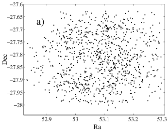
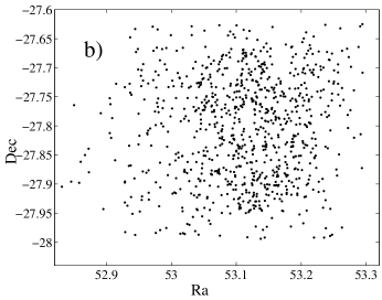
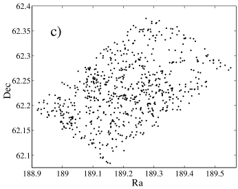
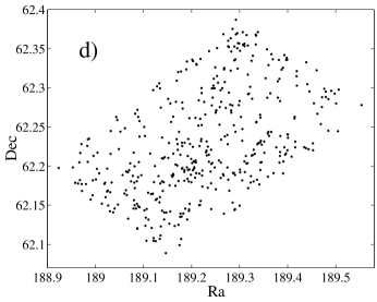
Figure 1.— The distribution of (a) 950 galaxies in the GOODS South with $0.47\leq z\leq 0.8$, (b) 882 galaxies with $0.9\leq z\leq 1.5$, (c) 685 galaxies in the GOODS North with $0.47\leq z\leq 0.8$, (d) 433 galaxies with $0.9\leq z\leq 1.5$. These are all projected in equatorial coordinates.

2. The Observed Samples

Our analysis is mainly based on the GOODS Catalogs using both its North and South components separately to check on its homogeneity and statistical uncertainty. The GOODS South Catalog has four components, the VVDS (VIMOS VLT Deep Survey) (Le Fèvre, et al., 2004), the ESO1 (Vanzella, et al., 2005), ESO2 (Vanzella, et al., 2006), and a spectroscopic redshift survey (Ravikumar, et al., 2007), all having spectra taken with VIMOS on the ESO VLT. These provide 1599, 234, 501, and 961 redshift determinations for each of the catalogs respectively. We cross correlate these with a 0.5 arc second search radius to eliminate multiple determinations of the same redshift. This leaves 950 distinct objects in the redshift range between 0.47 and 0.8 as well as 882 objects in the redshift range between 0.9 and 1.5. These ranges were selected to include a large enough number of galaxies for reasonable statistics in a small enough redshift band that evolution would be unlikely to dominate. This is clearly a compromise which could be improved in future larger but at least equally homogeneous catalogs. Figure 1 (a and b) shows these two redshift samples projected onto the sky.

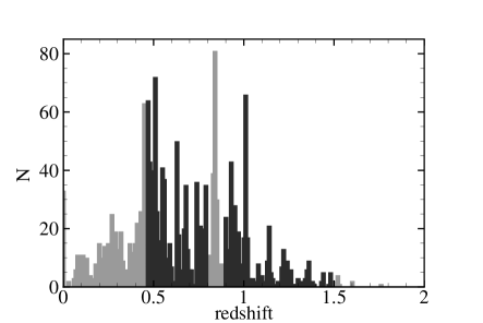
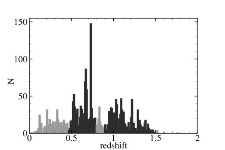
Figure 2.— The redshift distribution of galaxies in North (top) and South (bottom) catalogs. For each catalog, the galaxies in the redshift samples we use are shown as the dark filled histograms.

The GOODS North catalog contains a majority of objects from the Team Keck Treasury Redshift Survey (TKRS) (Wirth, et al., 2004). They measured spectroscopic redshifts of 1440 galaxies and AGNs (plus 96 stars) in this region. There are also 434 other redshifts in this region obtained by using the LRIS spectrograph (Oke, et al., 1995) on the twin 10 m telescopes of the W. M. Keck Observatory (Cohen, et al., 1996, 2000; Cowie, et al., 1996; Steidel, et al., 1996; Lowenthal, et al., 1997; Phillips, et al., 1997; Moustakas, Zepf & Davis, 1997; Cohen, 2001; Dawson, et al., 2001) and DEIMOS spectrograph (Faber, et al., 2003) on the Keck twin telescopes (Cowie, et al., 2004). These give a total of 1970 redshifts, of which 685 are between 0.47 and 0.80 and 433 are between 0.9 and 1.5, comparable with the numbers in these regions in the South catalog. Figure 1 (c and d) shows their distribution on the sky. Figure 2 shows the redshift distribution for the two ranges in the North and South, as well as for all redshifts in both regions. The mean redshifts of the four selected samples are 0.61 and 1.06 in the North, and 0.65 and 1.14 in the South.

In addition to illustrating the scales of the samples, figure (1) shows that they contain a range of voids, filamentary structures, underdense regions and clusters. It also shows the inhomogeneity of the South samples which contain four surveys. In particular, the GOODS South sample for high redshifts (figure (1b)) has an average density which increases systematically with increasing right ascension, even in this small area. The GOODS North sample, based mainly on one survey, is more homogeneous, allowing for greater fluctuations around its smaller average density.

3. The Galaxy Distribution Functions at $z\simeq 0.63$ and $z\simeq 1.1$

To obtain the distribution function, we map the galaxies onto a Hammer-Aitoff equal area projection (e.g. Calabretta & Greisen 2002), divide the area into square cells of a given angular size and count the number of galaxies in the volume projected into each cell. The samples are not yet large enough to examine the areas for completeness and statistical homogeneity in the usual ways (cf. Sivakoff & Saslaw 2005). However the consistency of our results below suggests that equation (1) will be a good representation of the actual distribution function.

Figure (3) shows examples of the resulting histograms for counts of galaxies in cells in the two redshift ranges of both the North and South Catalogs. The redshifts and cell sizes are labeled on the histograms. Other examples are similar, although as the cells become larger or the number of cells decreases, the fluctuations naturally increase. The solid line is the theoretical curve of equation (1) in which $\bar{N}$ is determined directly from the data. The value of $b$ may also be determined directly from the data using its relation to the variance of counts in cells having volume V projected onto the sky:

$$\langle(\Delta N)^{2}_{V}\rangle=\frac{\bar{N}}{(1-b(V))^{2}}.$$ (4)

Equation (4) is the variance of counts in cells and it follows either directly from equation (1) or from its moments, or from its generating function (see Saslaw 2000).

In addition, we can find $b$ using a least squares fit of equation (1) to the histograms. The values of $b$ for figure (3) obtained by least squares fitting are 0.17, 0.12, 0.15, 0.22 from left to right and top to bottom. In the Figures we use the values of $b$ from the observed variance of counts in cells. Thus the good agreement between observations and theory is obtained without the use of any free parameters.

Our results in figure (3), as well as previous observations of spatial and velocity distribution functions at low redshifts, are a challenge for the

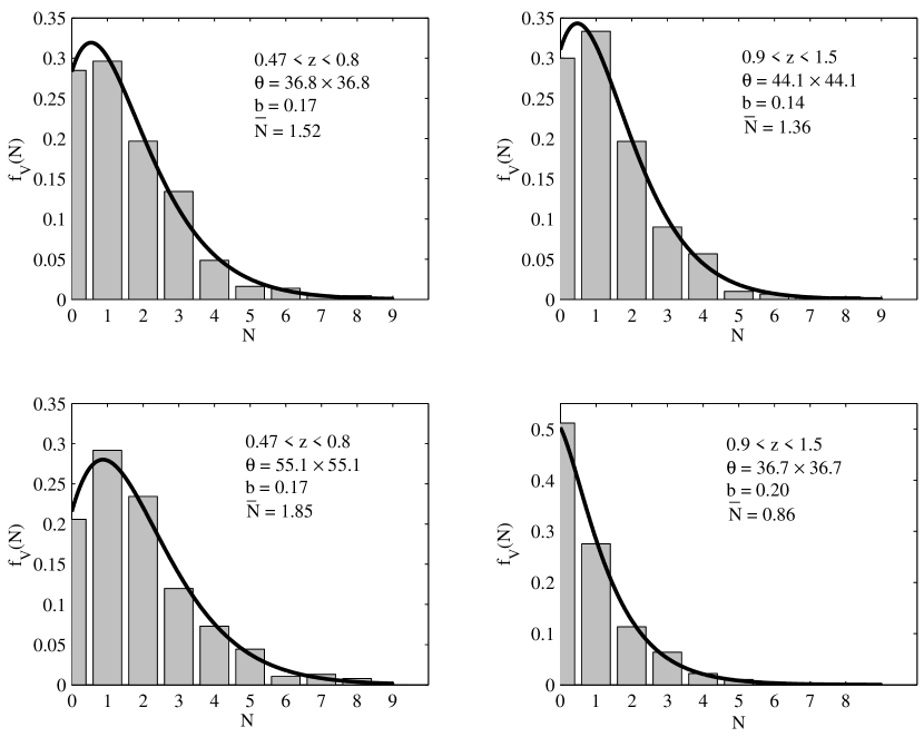
Figure 3.— Theoretical curve (continuous line) of $f_{V}(N)$ on the observed histograms for square cells of GOODS North (top) and GOODS South (bottom) for two redshift ranges.

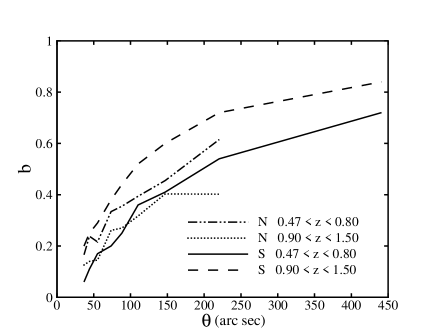
Figure 4.— The value of $b$ for cells of different angular sizes for the two redshift samples in the North and South GOODS catalogs.

Table 1 Properties of distribution functions from counts in cells.

$0.47\leq z\leq 0.8$						$0.9\leq z\leq 1.5$
	$b$	$\bar{N}$	$\theta$	$Physize$	n	$b$	$\bar{N}$	$\theta$	$Physize$	n
			($arcsec$)	$(kpc)$	(cells)			($arcsec$)	$(kpc)$	(cells)
	0.17	$1.52$	36.8	200	432	0.13	$0.95$	36.8	225	432
	0.24	$2.19$	44.1	240	300	0.14	$1.36$	44.1	270	300
	0.22	$3.42$	55.1	300	192	0.15	$2.13$	55.1	337	192
North	0.33	$6.08$	73.5	400	108	0.26	$3.79$	73.5	450	108
	0.36	$8.76$	88.2	480	75	0.27	$5.45$	88.2	540	75
	0.39	$13.69$	110.2	600	48	0.32	$8.52$	110.2	675	48
	0.46	$24.3$	147.0	801	27	0.40	$15.2$	147.0	900	27
	0.62	$54.75$	220.5	1201	12	0.40	$34.1$	220.5	1349	12
	0.06	$0.82$	36.7	205	864	0.20	$0.86$	36.7	226	864
	0.11	$1.18$	44.1	246	600	0.25	$1.20$	44.1	271	600
	0.17	$1.85$	55.1	308	384	0.29	$1.90$	55.1	339	384
	0.20	$3.30$	73.5	410	216	0.38	$3.40$	73.5	452	216
South	0.25	$4.70$	88.2	492	150	0.44	$4.90$	88.2	542	150
	0.36	$7.40$	110.2	615	96	0.52	$7.707$	110.2	677	96
	0.41	$13.10$	147.0	820	54	0.60	$13.70$	147.0	903	54
	0.54	$29.60$	220.5	1230	24	0.72	$30.80$	220.5	1355	24
	0.72	$118.30$	441.0	2460	6	0.84	$123.20$	441.0	2710	6

usual computer simulations to reproduce (without too many free parameters). For example, one of the important consequences of figure (3) is the role of galaxy mergers in altering their distribution function over time. From the viewpoint of the theory behind equation (1), the robustness of $f_{V}(N)$ to mergers can be understood analytically (Yang, Saslaw, Leong & Chan, 2008, in preparation).

4. The Observed Dependence of $b$  on Scale and Redshift

The value of $b$ is known to depend on the size of the cells for which it is measured. If cells are so small that they usually contain only zero or one galaxy, their counts-in-cells will have a nearly Poisson distribution for which $b\simeq 0$ and $\langle(\Delta N)^{2}\rangle\simeq\bar{N}$. Greater values of $b$ occur for larger departures from Poisson statistics, as equations (1) and (4) indicate. Another way of visualizing this is by relating $b$ to the two-galaxy correlation function:

$$b=-\frac{W}{2K}=\frac{2\pi Gm^{2}\bar{n}}{3T}\int_{V}\xi(\bar{n},T,r)\frac{1}{r}r^{2}dr$$ (5)

where $K$ is the kinetic energy and $T$ is the temperature given by the peculiar velocity dispersion relative to the average Hubble expansion. (For a detailed review see Saslaw 2000.) For larger volumes, there is a greater contribution of the two-galaxy correlation function $\xi(r)$ to the integral of the gravitational correlation energy $W$, and $b$ increases. On very large scales, the correlations become small and contribute no further to the integral in equation (5). Thus the value of $b$ reaches its asymptotic limit on these large scales, provided they are initially uncorrelated. At low redshifts, $b(r)$ in the 2MASS catalog can be used with equation (5) to determine the two-galaxy correlation function. Comparison of the result with the standard direct determination shows excellent agreement (Sivakoff & Saslaw, 2005).

The cell size $d(Mpc)$ is related to its angular size $\theta$(radians) at a redshift $z$ by (Coles & Lucchin, 2002)

$$\theta=\frac{H_{0}q^{2}_{0}}{c}~{}\frac{(1+z)^{2}}{\left[q_{0}z+(q_{0}-1)((1+2q_{0}z)^{0.5}-1)\right]}~{}d$$ (6)

where we take the Hubble constant $H_{0}=70$ $km$ $s^{-1}$ $Mpc^{-1}$ and $q_{0}=0.5$.

Figure (4) shows $b(\theta)$ for cells of different angular sizes (in arc seconds) for the two redshift samples in the North and South GOODS catalogs. Table (1) gives more detailed information on these results. This information is useful for understanding the physical scales of the cells and the numbers of galaxies and cells being analyzed. It also gives the numbers for figure (3) which are used to calculate the two-galaxy correlation function (in figure (5)) from equation (5). Notice that for the same angular size, the physical sizes of cells in the South is slightly greater than in the North, because of the slightly greater average redshift of the Southern samples. We have also examined the effect of the strong redshift peak in the South at $z=0.74$ by reducing the upper redshift to $z=0.73$ which eliminates the peak in that nearer sample. The result is to decrease the values of $b$ for the same size cells by between $0.01$ for the smallest cells and $0.1$ for cells of about $220$ arc sec in length, usually an effect of about $15-20$%.

Figure (5) compares $b(\theta)$ with values based on the two-galaxy angular correlation function, $W(s)$. Lahav & Saslaw 1992 derived $b(\theta)$ for square cells of size $\omega=\theta\times\theta$ deg²

$$b(\theta)=1-\left(1+\bar{N}s_{0}^{\gamma-1}C_{\gamma}\theta^{1-\gamma}\right)^{-1/2}$$ (7)

where $W(s)$ $=$ $(s/s_{0})^{1-\gamma}$, $\bar{N}$ is the expected number of galaxies in a cell, and $C_{\gamma}$ is a coefficient to be evaluated numerically. Lahav & Saslaw 1992 calculated $C_{\gamma}$’s corresponding to four different values of $\gamma=$ 1, 1.68, 1.8, and 2 to be 1, 1.87, 2.25, and 2.97 respectively. We used the lower redshift sample in the North (which seems the most homogeneous) and then fixed $C_{\gamma}$ to each of these four values to fit equation (7) to the data and find $\gamma$ and $s_{0}$. As table (2) shows by changing $C_{\gamma}$ to its four numerically calculated values the fitted values of $\gamma$ do not change but $s_{0}$ decreases.

To determine whether cells near the edges of each region could have significant effects on the results, we omitted them and found that they did not change the trend of the values of $b$ in the two redshift intervals.

We also tested the effects of different cross-correlation radii among the different catalogs which constitute the GOODS North and South catalogs. Increasing this cross-correlation radius from $0.5$ to $0.75$, $1.0$, and $1.5$ arcseconds gave $3009$, $3005$, $3003$ and $2994$ independent objects respectively. So cross-correlation radii in this range have negligible effects.

In the North Catalog, the majority of the data ($1536$ secure redshifts) come from the TKRS redshift survey, and the other $434$ are from other redshift surveys. To examine possible effects of differences among these catalogs, we repeated all the analysis using only the TKRS survey. This gave small changes in the values of $b$ but did not affect the trend of values of $b$ between the two redshift intervals.

As the total number of cells, $n$, in Table (1) decreases below about $150$ (conservatively) the $f_{V}(N)$ histograms become less smooth and their corresponding values of $b$ become less reliable. The only ways to explore these regimes more accurately are with large homogeneous samples covering greater areas, and with a larger number of such samples.

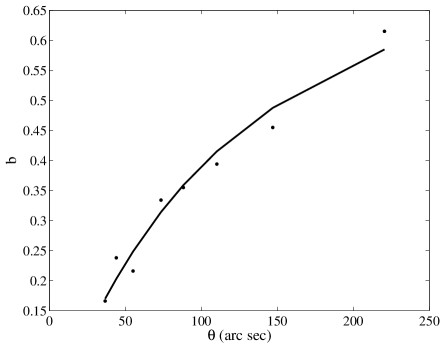
Figure 5.— The points show the $b$ values for different cell sizes in North with $0.47<z<0.8$. The curve is the predicted $b(\theta)$ fitted on these points according to $b(\theta)=1-\left(1+\bar{N}s_{0}^{\gamma-1}C_{\gamma}\theta^{1-\gamma}\right)^{-1/2}$(Lahav & Saslaw, 1992) with $s_{0}=0.0017^{\circ}$ and $\gamma=1.68$.

Table 2Two-point correlation function

$c_{\gamma}$	$\gamma$	$s_{0}$(degree)
1	1.68	0.0017
1.87	1.68	0.0007
2.25	1.68	0.0005
2.97	1.68	0.0003

5. Discussion

Our most striking result is that at redshifts up to about $z=1.5$ the form of the spatial galaxy distribution function is remarkably similar to its form at the present time. Both these forms were predicted by the gravitational statistical mechanics and thermodynamics of the cosmological many-body system. This indicates that although merging and dark matter can be important for the evolution of individual galaxies, they do not dominate the forms of the large scale galaxy distribution. The reasons for this lack of dominance may be able to place important constraints on merging and dark matter.

To obtain these constraints, we need to determine how $b(r,z)$ depends on the scale $r$, and how it evolves with redshift. The theory predicts both these dependencies (e.g. Saslaw 2000; Ahmad, Saslaw & Bhat 2002). In particular $b$ should decrease with increasing redshift. Figure (4) and Table (1) show that this decrease holds in the North GOODS catalog, but not in the South. The simplest explanation for this difference may be that the South region is a compilation of four distinct catalogs, none of which dominates. This may encourage more inhomogeneity than in the North region which is dominated by one catalog. Indeed Vanzella, et al. (2005, 2006) and Ravikumar, et al. (2007) have clearly noted the inhomogeneity of structure in the South region. This may be a region of excess clustering which would produce an unusually large apparent local value of $b$. (We recall that the usual value of $b$ represents an ensemble average over many regions which cover a representative range of clustering.) On the other hand, the decrease of $b$ with $z$ in the North region behaves qualitatively as expected. Whether it agrees quantitatively with the gravitational many-body theory is being investigated elsewhere (Yang, Saslaw, Leong & Chan (2008, in preparation)).

When $b(r)$ can be determined more accurately, using a larger number of larger homogeneous catalogs, it will also provide information on the evolution of the two-galaxy correlation function. (See Sivakoff & Saslaw 2005 for an example of the technique to accomplish this.) This, in turn, can then be related to many computer simulations of galaxy clustering which measure the two-galaxy correlations under a variety of conditions.

References

- Ahmad, Saslaw & Bhat (2002) Ahmad, F., Saslaw, W. C., & Bhat, N. I. 2002, ApJ, 571, 576
- Ahmad, Malik & Masood (2006) Ahmad, F., Malik, M. A., & Masood, S. 2006, IJMPD, 15, 1267
- Calabretta & Greisen (2002) Calabretta, M. R. & Greisen, E. W. 2002, A&A, 395, 1077
- Cohen, et al. (1996) Cohen, J. G., Cowie, L. L., Hogg, D. W., Songaila, A., Blandford, R., Hu, E. M., & Shopbell, P. 1996, ApJ, 471, L5
- Cohen, et al. (2000) Cohen, J. G., Hogg, D. W., Blandford, R., Cowie, L. L., Hu, E. M., Songaila, A., Shopbell, P., & Richberg, K. 2000, ApJ, 538, 29
- Cohen (2001) Cohen, J. G., 2001, AJ, 121, 2895
- Coles & Lucchin (2002) Coles, P., Lucchin, F., 2002, COSMOLOGY: The Origin and Evolution of Cosmic Structure, John Wiley & Sons, Ltd
- Cowie, et al. (1996) Cowie, L. L., Songaila, A., Hu, E. M., Cohen, J. G. 1996, AJ, 112, 839
- Cowie, et al. (2004) Cowie, L. L., Barger, A. J., Hu, E. M., Capak, P. 2004, AJ, 127, 3137
- Crane & Saslaw (1986) Crane, P.,& Saslaw, W. C. 1986, ApJ, 301, 1
- Dawson, et al. (2001) Dawson, S., Stern, D., Bunker, A. J., Spinard, H.,& Dey, A. 2001, AJ, 122, 598
- Faber, et al. (2003) Faber, S. M., et al. 2003, SPIE, 4841, 1657
- Fang & Zou (1994) Fang, F., & Zou, Z. 1994, ApJ, 421, 9
- Guo & White (2008) Guo, Q., & White, S. D. M. 2008, MNRAS, 384, 2
- Lahav & Saslaw (1992) Lahav, O., & Saslaw, W. C. 1992, ApJ, 396, 430
- Le Fèvre, et al. (2004) Le Fèvre, O., et al. 2004, A&A, 428, 1043
- Leong & Saslaw (2004) Leong, B., & Saslaw, W. C. 2004, ApJ, 608, 636
- Lowenthal, et al. (1997) Lowenthal, J. D., et al. 1997, ApJ, 481, 673
- Moustakas, Zepf & Davis (1997) Moustakas, L. A., Zepf, S. E., & Davis, M. 1997, in The Hubble Space Telescope and the High-Redshift Universe, ed. N. Tanvir, A. Aragon-Salamanca, & J. Wall (Singapore: World Scientific), 273
- Oke, et al. (1995) Oke, J. B., et al. 1995, PASP, 107, 135
- Phillips, et al. (1997) Phillips, A. C., 1997, ApJ, 489, 543
- Ravikumar, et al. (2007) Ravikumar, C. D., et al. 2007, A&A, 465, 1099
- Saslaw & Hamilton (1984) Saslaw, W. C., & Hamilton, A. J. S. 1984, ApJ, 276, 13
- Saslaw (1986) Saslaw, W. C. 1986, ApJ, 304, 11
- Saslaw & Fang (1996) Saslaw, W. C., & Fang, F. 1996, ApJ, 460, 16
- Saslaw & Haque-Copilah (1998) Saslaw, W. C., & Haque-Copilah, S. 1998, ApJ, 509, 595
- Saslaw & Edgar (2000) Saslaw, W. C., & Edgar, J. H. 2000, ApJ, 534, 1
- Saslaw (2000) Saslaw, W. C., 2000, The Distribution of the Galaxies: Gravitational Clustering in Cosmology, (New York: Cambridge University Press)
- Saslaw (2008) Saslaw, W. C. 2008, in Dynamics and Thermodynamics of Systems with Long-Range Interactions: Theory and Experiments ed. by A. Campa, A. Giansanti, G. Morigl & F. Sylos Labini (New York: American Institute of Physics Conference Proceedings #970)
- Sivakoff & Saslaw (2005) Sivakoff, G. R., & Saslaw, W. C. 2005, ApJ, 626, 795
- Steidel, et al. (1996) Steidel, C. C., Giavalisco, M., Dickinson, M., Adelberger, K. L. 1996, AJ, 112, 352
- Vanzella, et al. (2005) Vanzella, E., et al. 2005, A&A, 434, 53
- Vanzella, et al. (2006) Vanzella, E., et al. 2006, A&A, 454, 423
- Wirth, et al. (2004) Wirth, G. D. , et al. 2004, AJ, 127, 3121
- Yang, Saslaw, Leong & Chan (2008, in preparation) Yang, Saslaw, Leong & Chan (2008, in preparation)