Ergodic and non-ergodic anomalous diffusion in coupled stochastic processes

Abstract

Inspired by problems in biochemical kinetics, we study statistical properties of an over-damped Langevin process whose friction coefficient depends on the state of a similar, unobserved process. Integrating out the latter, we derive the long time behaviour of the mean square displacement. Anomalous diffusion is found. Since the diffusion exponent can not be predicted using a simple scaling argument, anomalous scaling appears as well. We also find that the coupling can lead to ergodic or non-ergodic behavior of the studied process. We compare our theoretical predictions with numerical simulations and find an excellent agreement. The findings caution against treating biochemical systems coupled with unobserved dynamical degrees of freedom by means of standard, diffusive Langevin descriptions.

1 Introduction

Single molecule kinetics has come within reach of biophysical experiments [1, 2, 3], and theoretical and computational tools for analysis of such processes have experienced a corresponding growth [4, 5, 6, 7, 8]. It is clear that the combinatorially large number of microscopic steps involved in even the simplest of biochemical events makes their rigorous stochastic treatment difficult. For example, gene expression, often modeled as a single-step mRNA creation, in fact, includes transcription-factor-DNA binding, polymerase recruitment, transcriptional bubble formation, and multiple elongation steps, each of which is a complex process on its own.

Therefore, any theoretical analysis of stochastic biochemical processes necessarily involves coarse-graining: identifying a small subset of dynamical variables that are modeled explicitly, while agglomerating the rest into an effective behaviour. Such coarse-grained dynamics is often modeled using the master equation or the Langevin approaches, which require Markoviness or white-noise random forcing. Both of these assumptions are, generally, flawed, and quantitative corrections have been worked out in certain cases [9, 10]. Less explored is the possibility that internal degrees of freedom can introduce qualitative differences, such as long-range temporal correlations among state transitions and non-diffusive behaviour of the observed quantities.

A well-studied example shows that this is possible for a random walk on a discrete lattice. In Ref. [11], Weiss and Havlin analyzed a two-dimensional diffusion model, known as the comb model. There dynamics along the $y$ coordinate is unlimited, while motion along $x$ is allowed only when $y=0$. This results in $\langle x\rangle=0$ and $\langle x^{2}\rangle\propto\sqrt{t}$, that is, in a sub-diffusive motion of $x$. This model is hardly realistic in a biochemical context due to the discontinuous dependence of the diffusion coefficient on $y$. However, it is plausible that diffusive dynamics of a real biological or chemical variable in the state space or in the physical space depends on unobserved, decimated variables in some other non-trivial way. For example, in a chemotaxing E. coli, the number of unobserved signaling proteins CheY-P is coupled to the distribution of times a bacterial motor rotates counterclockwise, and the bacterium swims straight. For a fixed concentration of CheY-P, obtained by modifying the chemotaxis network, the distribution is essentially exponential [12], resulting in a regular diffusive motion of the bacterium. But in a wild-type bacterium, as the number of CheY-P fluctuates (diffuses in the number space even for a constant external signal), the distribution becomes a power law, and bacteria exhibit super-diffusive real-space motion. While not true in this particular system, the distribution of clockwise rotation times could have been strongly coupled to CheY-P as well. This would have resulted in a power law distribution of times that the bacterium spends reorienting itself without moving forward, and hence in its sub-diffusive motion. In both cases, neglecting the CheY-P fluctuations and describing bacterial motion as a normal diffusion is qualitatively wrong.

In this paper, we abstract out the detailed biology and explore these types of phenomena from the point of view of statistical physics. We derive the properties of a diffusion process, for which the diffusion coefficient depends on the state of another, unobserved, variable. We show that, quite generally, such dependence leads to anomalous diffusion of the observed process, suggesting that traditional stochastic approaches may fail, and that more thought should be given to modeling stochastic phenomena in complex interacting systems, in particular in biophysics.

2 The Model

Our model is described by two variables $x$ and $y$, which may represent, in particular, concentrations of two interacting chemical species. The $x$ is considered as the observed quantity, while $y$ is assumed hidden (i.e., unobserved). Particles of both species can be created and destroyed, which results in an over-damped diffusive motion of the system in the concentration space (we disregard the directional drift for simplicity, but it can be reintroduced easily). We assume that the diffusion of $x$ is $y$-dependent. That is,

$$\frac{dy}{dt} =\frac{1}{\gamma_{y}}\eta\left(t\right),$$ (1)

$$\frac{dx}{dt} =\frac{C\left(y\right)}{\gamma_{x}}\xi\left(t\right).$$ (2)

Here $\gamma_{x},\gamma_{y}$ are the effective friction coefficients (assumed to be homogeneous) corresponding to $x,y$; $\eta\left(t\right)$ and $\xi\left(t\right)$ are independent, zero-mean white noise forces such that

$$\langle\eta\left(t\right)\eta\left(t^{\prime}\right)\rangle =2D_{y}\gamma_{y}^{2}\delta\left(t-t^{\prime}\right),$$ (3)

$$\langle\xi\left(t\right)\xi\left(t^{\prime}\right)\rangle =2D_{x}\gamma_{x}^{2}\delta\left(t-t^{\prime}\right).$$ (4)

The idea of multiplicative noise was explored before. In [13] the authors considered the case of a Langevin process (not over-damped), in which a function of the velocity serves as a “filter” for the white noise. In [14] the multiplicative noise enters as a random friction coefficient; however, the distribution of the random friction is independent of time. Similarly in [15] the noise enters as a random mass with distribution which is again independent of time. Our model is different from the above mentioned models since the distribution of the random coupling parameter $C(y)$ is time dependent; moreover it depends in an arbitrary way (through the function $C(y)$) on another variable, which diffuses and hence has long range temporal correlations. Further, the coupling considered in our model does not introduce a directional bias since it is multiplied by a white noise $\xi$, which takes both positive and negative values.

The PDF of $y$ is that of a normal diffusion

$$p\left(y,t|y_{0},0\right)=\frac{1}{\sqrt{4\pi D_{y}t}}e^{-\frac{(y-y_{0})^{2}}{4D_{y}t}},$$ (5)

where the initial condition is $y(t=0)=y_{0}$.

The dynamics of the mean square displacement (MSD) $\langle x\left(t\right)^{2}\rangle$, where $\langle\cdots\rangle$ stands for the average over the white noises $\eta$ and $\xi$, can be derived. Formally integrating Equation (2) and substituting it in the expression for the derivative of $x^{2}$ yields,

$$\frac{dx\left(t\right)^{2}}{dt}=\frac{2C\left(y\right)}{\gamma_{x}^{2}}\xi\left(t\right)\int_{0}^{t}C\left(y\left(t^{\prime}\right)\right)\xi\left(t^{\prime}\right)dt^{\prime}.$$ (6)

Averaging over the noise $\xi(t)$ yields the dynamics of the MSD of $x$ conditional on $y(t)$,

$$\frac{d\langle x\left(t\right)^{2}|y(t)\rangle}{dt}=2D_{x}C(y(t))^{2}.$$ (7)

To get the marginal expectation $\langle x\left(t\right)^{2}\rangle$, we now average the conditional expectation over $y$, which is distributed as in Equation (5):

$$\frac{d\overline{\langle x(t)^{2}\rangle}}{dt}=\frac{2D_{x}}{\sqrt{4\pi D_{y}t}}\int_{-\infty}^{\infty}e^{-\frac{(y-y_{0})^{2}}{4D_{y}t}}C(y(t))^{2}dy.$$ (8)

The function $C(y)$ may take different forms for different systems. The simplest case is when the dynamics of $x$ is independent of $y$ and $C\left(y\right)=C={\rm const}$. Substituting this in Equation (8) yields the expected trivial result $\overline{\langle x^{2}\rangle}=2D_{x}C^{2}t$.

Another scenario is that $x$ can evolve in time only for a given range of $y$ values ($|y|<y_{1}$), which resembles the discrete comb model of Weiss and Havlin [11]. Notice, however, that the comb model is based on geometric constraints, i.e., the teeth, while in our case the coupling between the two process is not due to the topology, but rather to the physical nature of the processes. The similarity arises due the fact that in both models the first passage time distribution in the infinitely long $y$ axis, dominate the dynamics. Indeed, substituting $C(y(t))=C\Theta\left(y_{1}-y\left(t\right)\right)\Theta\left(y_{1}+y\left(t\right)\right)$, where $C$ is a dimensionless constant, and $\Theta(y)$ is the Heaviside Theta function, into Equation (8), we see that, for $t\gg y_{1}^{2}/\left(12D_{y}\right)$, $\overline{\langle x\left(t\right)^{2}\rangle}\sim\sqrt{t}$ in agreement with [11]. If $C(y)$ falls off exponentially as $y\to\infty$, the same sub-diffusion exponent is recovered.

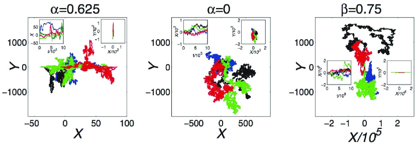
Figure 1: Typical trajectories for different forms of the coupling function $C(y)$. We set $D_{x}=D_{y}=\gamma_{x}=\gamma_{y}=A=1$. In the left panel we used the repressive coupling of Equation (9) with $\alpha=0.625$ to illustrate the suppression of diffusion in $x$. The central panel shows the case of $\alpha=0$ in Equation (9), namely decoupled Langevin processes resulting in normal diffusion. The right panel shows the case of enhanced diffusion in $x$ due to coupling of the form of Equation (18) with $\beta=0.75$. In each of the panels the left inset shows the observable $x$ as a function of time and the right inset shows $x$ and $y$ scaled equally. All trajectories start at $x=y=0$. The time step is set to $1$ and the total duration of each trajectory is $10^{6}$.

A more interesting case is when, at large $y$, $C(y)$ falls off, but not too sharply. We consider a power law form, namely

$$C(y(t))=\frac{1}{1+|Ay|^{\alpha}},$$ (9)

where $A$ is a constant with the units of inverse length, and $\alpha$ is a dimensionless parameter. This is of a form of a repressive, cooperative Hill kinetics, which describes many biochemical processes [16]. Typical diffusive trajectories with this $C(y)$, $A=1$, and $\alpha=0,0.625$ are shown in Figure 1.

Assuming that the behaviour of $C(y)$ for large $y$ (i.e., $C(y)\sim|y|^{-\alpha}$) dominates the $t\to\infty$ dynamics of $\overline{\langle x(t)^{2}\rangle}$, a simple scaling argument suggests that $\overline{\langle x\left(t\right)^{2}\rangle}\sim t^{1-\alpha}$. However, this is clearly wrong for large $\alpha$, suggesting that $\overline{\langle x\left(t\right)^{2}\rangle}$ must pick up an anomalous scaling due to the $y\to 0$ properties of $C(y)$. In what follows, we derive the long time behaviour of $\overline{\langle x\left(t\right)^{2}\rangle}$ in a more rigorous way.

Equation (8) with $C(y)$ as in Equation (9), and considering the long time limit (${y_{0}}/{\sqrt{4D_{y}t}}\ll 1$) gives

$$\frac{d\overline{\langle x(t)^{2}\rangle}}{dt}=\frac{4D_{x}}{\sqrt{\pi}}\left\{\displaystyle{\int_{0}^{\frac{1}{A\sqrt{4D_{y}t}}}}\frac{e^{-y^{2}}}{\left[1+\left(\sqrt{4D_{y}t}Ay\right)^{\alpha}\right]^{2}}dy\right.\left.+{\displaystyle{\int_{\frac{1}{A\sqrt{4D_{y}t}}}^{\infty}}}\frac{e^{-y^{2}}}{\left[1+\left(\sqrt{4D_{y}t}Ay\right)^{\alpha}\right]^{2}}dy\right\}.$$ (10)

In the first integral, we approximate the integrand as a constant for $t\to\infty$, and, in the second integral, we neglect $1$ compared to $\left(\sqrt{4D_{y}t}\,|Ay|\right)^{\alpha}$, thus obtaining

$$\frac{d\overline{\langle x^{2}\rangle}}{dt}\approx\frac{2D_{X}}{A\sqrt{\pi D_{y}t}}+\frac{2D_{x}t^{-\alpha}}{\left(4A^{2}D_{y}\right)^{-\alpha}\sqrt{\pi}}\Gamma\left(\frac{1}{2}-\alpha,\frac{1}{4A^{2}D_{y}t}\right),$$ (11)

where $\Gamma\left(a,b\right)\equiv{\int_{b}^{\infty}}\tau^{a-1}e^{-\tau}d\tau$ is the incomplete Gamma function. Integrating Equation (11) over $t$ results in the long time behaviour of $\overline{\langle x(t)^{2}\rangle}$

$$\overline{\langle x(t)^{2}\rangle}\sim D_{1}\sqrt{t}+D_{2}t^{1-\alpha},$$ (12)

where $D_{1,2}$ are constants depending on the model parameters $D_{x}$, $D_{y}$, $\alpha$ and $A$. This implies that, for $\alpha<1/2$, the long time behaviour is dominated by $\overline{\langle x(t)^{2}\rangle}\sim t^{1-\alpha}$, as the scaling argument suggests. However, for $\alpha>1/2$, the scaling argument breaks and $\overline{\langle x(t)^{2}\rangle}\sim\sqrt{t}$. Note that when the $C\left(y\right)$ falls faster than $1/\sqrt{y}$, the diffusion exponent is exactly the same as in the case in which the dynamics of $x$ is limited to a finite range near $y=0$.

The case of $\alpha=\frac{1}{2}$ is special and the integral of Equation (10) can be calculated exactly, yielding

$$\frac{d\overline{\langle x(t)^{2}\rangle}}{dt}=G^{5\ 4}_{4\ 5}\left(\frac{1}{4A^{2}D_{y}t}\left|\begin{array}[]{c}-\frac{1}{4},0,\frac{1}{4},\frac{1}{2}\\ 0,0,\frac{1}{4},\frac{1}{2},\frac{3}{4}\end{array}\right.\right)\sim\frac{\ln t}{\sqrt{t}},$$ (15)

where $G$ denotes the Meijer G function [17]. The leading order term of the MSD is then

$$\overline{\langle x(t)^{2}\rangle}\sim\sqrt{t}\ln t.$$ (16)

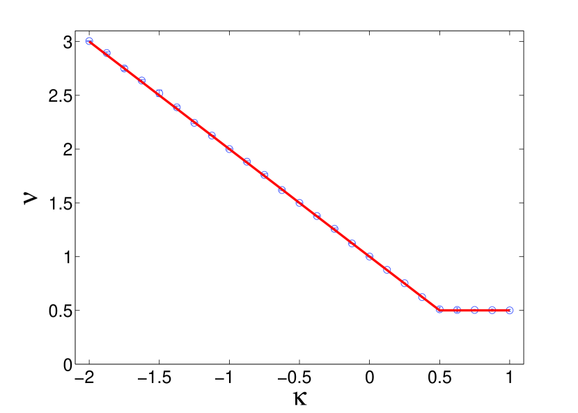
Figure 2: Leading order diffusion exponent $\nu$ defined by $\overline{\langle x(t)^{2}\rangle}\sim t^{\nu}$ for the coupled stochastic processes model with different couplings between the diffusion of $x$ and $y$, measured by the exponent $\kappa$. For the case of hindered diffusion of $x$, Equation (9), $\kappa=\alpha$, while for the enhanced diffusion, Equation (18), $\kappa=-\beta$. Numerical simulations (points) and theoretical predictions (line) agree for both scenarios.

The coupling function $C(y)$ depends only on the variable $y$ which undergoes normal diffusion. Thus we can derive the probability distribution of $C(y)$. In order to simplify the notation, in what follows we use $C$ to denote the coupling function without explicitly specifying its dependence on $y$. When $C$ is given by Equation (9), its probability density is:

$$P\left(C\right)=\frac{2}{\alpha C^{\frac{\alpha+1}{\alpha}}\left(1-C\right)^{\frac{\alpha-1}{\alpha}}A\sqrt{4\pi D_{y}t}}e^{-\frac{\left(1-C\right)^{2/\alpha}}{4D_{y}tA^{2}C^{\frac{2}{\alpha}}}},$$ (17)

where $0\leq C\leq 1$. In the above derivation, we set $y(t=0)=0$ for simplicity. We see that the distribution of the noise introduced by $C$ is time dependent. Note that the temporal correlations of $C$ are also important for the dynamic properties of $x$.

So far we have considered only situations in which the motion of $x$ was slowed at large $y$, but we can also consider the opposite scenarios, when large $y$ promotes diffusion in $x$, as in [12]:

$$C\left(y(t)\right)=|Ay|^{\beta},\quad\beta>0.$$ (18)

This now resembles the Hill activation kinetics for low concentration of the substrate molecules [16]. Typical trajectories for this form of the coupling function with $\beta=0.75$ are shown in Figure 1.

For coupling of this form, the dynamics of the MSD(Equation (8)) yields

$$\frac{d\overline{\langle x(t)^{2}\rangle}}{dt}=\frac{2D_{x}}{\sqrt{\pi}}\left(4D_{y}t\right)^{\beta}\int_{-\infty}^{\infty}e^{-\left(y-\frac{y_{0}}{\sqrt{4D_{y}t}}\right)^{2}}|Ay|^{2\beta}dy,$$ (19)

which, in the long time limit, gives ${d\overline{\langle x(t)^{2}\rangle}}/{dt}\sim t^{\beta}$, and

$$\overline{\langle x(t)^{2}\rangle}\sim t^{\beta+1}.$$ (20)

The distribution of the coupling function $C$ in this case is given by

$$P\left(C\right)=\frac{C^{-\frac{\beta-1}{\beta}}e^{-\frac{C^{2/\beta}}{4t}}}{\sqrt{\pi}\sqrt{t}\beta},$$ (21)

where $C\geq 0$.

To confirm our analytical results, we performed numerical simulations for the different cases considered above. In Figure 2, we present a comparison of the diffusion exponent $\nu$ (defined by $\overline{\langle x(t)^{2}\rangle}\sim t^{\nu}$) versus the coupling parameter $\kappa$ (for the sub-diffusion scenario, Equation (9), $\kappa=\alpha$, and for the super-diffusion scenario, Equation (18), $\kappa=-\beta$) between the simulations and the analytical results. The simulations where done according to Eqs. (1, 2) with $\gamma_{x,y}=1$, $D_{x,y}=1$ and $dt=1$. We averaged the results over $10^{4}$ trajectories, each of duration $10^{7}\dots 10^{8}dt$.

A simple linear regression to $\log\overline{\langle x(t)^{2}\rangle}=\nu\log t+{\rm const}$ was performed to estimate $\nu$. Since the standard parameter errors obtained for the regressions were negligible, the error bars of $\nu$ were estimated from the variability of the fitted values as we changed the domain of $t$, for which the fits were performed. Figure 2 shows a clear agreement between our theoretical results and the simulations. Note that, in certain cases, the convergence to the leading behaviour of $\overline{\langle x(t)^{2}\rangle}$ as $t\to\infty$ is slow since the difference between the exponents of the leading and the sub-leading terms is small. This slowness determined the lengths of the simulations.

3 Time Averaged Mean Square Displacement

There are many models of anomalous diffusion, including a time dependent friction coefficient in the Langevin equation [18], continuous time random walk (CTRW) [19], fractional Brownian dynamics [20], fractional Langevin dynamics [21, 22, 23] and Langevin dynamics with coloured noise [24], to name a few. For a new model resulting in an anomalous diffusion, it is important to see if it can be reduced to one of these more familiar constructions. For example, the $t\to\infty$ behaviour of the original comb model is equivalent to CTRW [25] with a power-law tail of the distribution of the times between successive jumps along $x$. However, in our model, the analogy is not as straightforward since the continuous dynamics of $y$ induces temporal correlations among successive motions along $x$.

To understand the relation of the coupled diffusion model to the others in the literature, we note that all of them yield the same behaviour for the ensemble averaged MSD in the long time limit. However, they still differ from each other in the short time behaviour, the shape of the distribution, and even in the long time behaviour of time averaged quantities (for example, the CTRW exhibits ergodicity breaking [26]). In particular, the time averaged MSD (TAMSD) is an important property (it is the TAMSD that is observed in typical single molecule diffusion experiments in biological systems [3, 27], and the number of recorded trajectories is often insufficient to estimate ensemble averages).

The TAMSD is defined as

$$\overline{\delta^{2}}\left(\Delta,t\right)=\frac{1}{t-\Delta}\displaystyle{\int\limits_{0}^{t-\Delta}}\left[x\left(\tau+\Delta\right)-x\left(\tau\right)\right]^{2}d\tau,$$ (22)

which averages the squared displacement of a particle in time $\Delta$ (the time lag) over a single particle trajectory of duration $t$. For CTRW, the TAMSD is a random quantity and even its ensemble average still exhibits aging, that is, dependence on the measurement duration [28, 29] $t$ in Equation (22). On the contrary, for the fractional Brownian and Langevin dynamics, the TAMSD converges to the ensemble average MSD for long times [30].

We investigated the behaviour of the TAMSD in our model with repressive coupling numerically. We find that, when the scaling argument holds, namely for $\alpha\leq 1/2$ (see Equation (9)), the TAMSD is not a random quantity, but it still shows aging, as we would expect for Langevin dynamics with a time dependent friction. On the other hand, when $\alpha\geq 1/2$, and the diffusion exponent is $\nu=1/2$, the TAMSD shows a similar behaviour to that of the CTRW [28]. In Figure 3, we show the TAMSD versus the time lag $\Delta$ for $\alpha=0.75$ and $\alpha=0.25$. Each line shows the TAMSD for a single trajectory. The solid red lines represent trajectories of duration $t=10^{5}$, and the dashed blue lines are for $t=10^{6}$. All lines show a linear dependence on $\Delta$, but with different coefficients. For $\alpha=0.25$, the TAMSD lines converge as the trajectory duration grows (the dashed blue lines essentially overlap), while for $\alpha=0.75$, the lines remain random. This is a clear indication of ergodicity breaking in our model for $\alpha>0.5$. Further, this analysis suggests that the coupled Langevin processes model stands as its own class among other anomalous diffusion models, exhibiting time-dependent diffusion coefficient Langevin dynamics for certain forms of coupling, and some aspects of ergodicity-breaking CTRW for others.

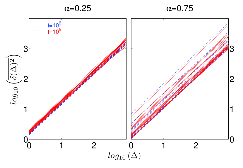
Figure 3: The time averaged MSD $\overline{\delta^{2}}\left(\Delta,t\right)$ versus $\Delta$ for $\alpha=0.25,0.75$ (left and right panels, respectively). All other parameters are the same as for the previous figures. We used 20 trajectories of duration $t=10^{5}$ (solid red lines) and 20 trajectories of duration $t=10^{6}$ (dashed blue lines). The straight lines with slope $1$ in the log-log scale reflect a linear dependence of the TAMSD on the time lag $\Delta$. For $\alpha=0.25$, the TAMSD of different trajectories converges as the measurement time increases (the blue lines collapse, and the red do not), namely a time average of a single particle behaves like the ensemble average. However, for $\alpha=0.75$, there is no such convergence, just like for CTRW (the coefficient of proportionality between $\overline{\delta^{2}}$ and $\Delta$ varies from trajectory to trajectory). In both cases, the ensemble average of the TAMSD decreases as the measurement time increases, indicating aging.

4 Discussion

In this article, we introduced a model of coupled diffusive processes, where the diffusion of the observed variable $x$ is coupled to the value of a hidden variable $y$. We showed that the dynamics of $x$ exhibits anomalous diffusion for every considered form of the coupling between the variables. Depending on the nature of the coupling, the motion of $x$ can be sub- or super-diffusive (and even super-ballistic, as is the case of a frictionless particle subject to a white noise). Further, even for an arbitrary “strong” (such that the dynamics of $x$ is limited to a small range of $y$ values) repressive $xy$ coupling, the $x$ diffusion exponent $\nu$ is limited from below by $\frac{1}{2}$ (anomalous scaling), so that localization of $x$ is impossible. Even though the long-time ensemble-averaged behaviour of our model is similar to that of many others describing anomalous diffusion, the model does not reduce to any of them, exhibiting an effective time-dependent diffusion coefficient, aging, and ergodicity breaking for different values of its parameters.

The anomalous scaling and the ergodicity breaking appear for “strong” $xy$ coupling (i.e., large $\alpha$). This is because, for $\alpha<1/2$, motion of particles away from $y=0$ contributes substantially to the ensemble averaged MSD of $x$. On the contrary, for $\alpha>1/2$, only motion near $y=0$ is important, namely the first passage time in an infinite one dimensional system (the diffusion process in $y$) plays a major role in the dynamics of the observed quantity, $x$. It was also verified numerically that, for $\alpha>1/2$, where the dynamics of $x$ is dominated by motion in a narrow range near $y=0$, the propagator is non-Gaussian as expected from a CTRW-like renewal process. A similar result holds for the super-diffusive regime, $\beta>0$. On the other hand when the motion at any $y$ is important ($0\leq\alpha<1/2$), the process in $x$ has long-time correlations and the propagator takes a Gaussian form (similar to that of a diffusion process with a time dependent diffusion coefficient).

While important in its own right, the coupled diffusion model raises its most important questions in the biological domain. Unobserved dynamical quantities lead to anomalous diffusion in E. coli chemotaxis [12], or in mRNA diffusion in cells [3]. Further, some of the best established models of cellular regulation involve coarse-graining of dynamics. For example, in some models of the E. coli lac operon, the lac repressor itself is an unobserved variable [31], which is coupled to the speed of production of the lactose permease and the lactose-utilizing enzyme and, through them, to the import and the degradation of lactose in the cell. Since any coupling may lead to anomalous diffusion and in some cases even to ergodicity breaking, it begs the question whether relying on the common Langevin or master equation analysis of stochasticity of the lac repressor or other regulatory circuits, such as the $\lambda$-phage [4, 8], mar [1], and others, is rigorously justifiable.

References

References

- [1] C. C. Guet et al. Minimally invasive determination of mrna concentration in single living bacteria. Nucleic Acids Research, 36(12):e73, 2008.
- [2] B. P. English et al. Ever-fluctuating single enzyme molecules: Michaelis-menten equation revisited. Nature Chemical Biology, 2(2):87, 2006.
- [3] I. Golding and E. C. Cox. Physical nature of bacterial cytoplasm. Phys. Rev. Lett., 96:098102, 2006.
- [4] Harley H. McAdams and Adam Arkin. Simulation of prokaryotic genetic circuits. Annu. Rev. Biophys. Biomol. Struct., 27:199–224, 1998.
- [5] J Paulsson. Summing up the noise in gene networks. Nature, 427:415–418, 2004.
- [6] NA Sinitsyn, N Hengartner, and I Nemenman. Coarse-graining stochastic biochemical networks: quasi-stationary approximation and fast simulations using a stochastic path integral technique. submitted to Proc. Nat. Ac. Sci., 2008.
- [7] Masaki Sasai and Peter G. Wolynes. Stochastic gene expression as a many-body problem. Proc. Natl. Ac. Sci. USA, 100(5):2374–2379, 2003.
- [8] E. Aurell and K. Sneppen. Epigenetics as a first exit problem. Physical Review Letters, 88(4):048101, 2002.
- [9] I. V. Gopich and A. Szabo. Theory of the statistics of kinetic transitions with application to single-molecule enzyme catalysis. The Journal of Chemical Physics, 124(15):154712, 2006.
- [10] N. A. Sinitsyn and I. Nemenman. The berry phase and the pump flux in stochastic chemical kinetics. EPL (Europhysics Letters), 77(5):58001, 2007.
- [11] G. H. Weiss and S. Havlin. Some properties of a random walk on a comb structure. Physica A, 134(2):474–482, 1986.
- [12] E. Korobkova et al. From molecular noise to behavioural variability in single bacterium. Nature, 428:574, 2004.
- [13] I. Lubashevsky, R. Friedrich, and A. Heuer. Realization of levy walks as markovian stochastic process. Physical Review E, 79:011110, 2009.
- [14] Christian Beck. Dynamical foundations of nonextensive statistical mechanics. Phys. Rev. Lett., 87(18):180601, Oct 2001.
- [15] M. Ausloos and R. Lambiotte. Brownian particle having a fluctuating mass. Phys. Rev. E, 73:011105, 2006.
- [16] Bruce Alberts, Alexander Johnson, Peter Walter, Julian Lewis, Martin Raff, and Keith Roberts. Molecular Biology of the Cell. Garland Science, 5th edition, 2007.
- [17] S. Wolfram. The mathematica Book. Cambridge University press, Cambridge, 4 edition, 1999.
- [18] J. Luczka, P. Talkner, and P. Hanggi. Diffusion of brownian particles goverened by fluctuating friction. Physica A, 278:18–31, 2000.
- [19] H. Sher and E. W. Montroll. Anomalous transit-time dispersion in amorphous solids. Physical Review B, 12:2455, 1975.
- [20] Benoit B. Mandelbrot and John W. Van Ness. Fractional brownian motions, fractional noises and applications. SIAM Review, 10(4):422–437, 1968.
- [21] Wei Min, Guobin Luo, Binny J. Cherayil, S. C. Kou, and X. Sunney Xie. Observation of a power-law memory kernel for fluctuations within a single protein molecule. Phys. Rev. Lett., 94(19):198302, 2005.
- [22] I. Goychuk and P. Hänggi. Anomalous escape governed by thermal 1/f noise. Physical Review Letters, 99(20):200601, 2007.
- [23] S. Burov and E. Barkai. Critical exponent of the fractional langevin equation. Physical Review Letters, 100(7):070601, 2008.
- [24] R. Muralidhar, D. Ramkrishna, H. Nakanishi, and D. Jacobs. Anomalous diffusion: A dynamic perspective. Physica A, 167:539–559, 1990.
- [25] J. P. Bouchaud and A. Georges. Anomalous diffusion in disordered media: Statistical mechanisms, models and physical applications. Physics Reports, 195:127, 1990.
- [26] G. Bel and E. Barkai. Ergodicity breaking in continuous time random walk. Phys. Rev. Lett., 94:240602, 2005.
- [27] I. M. Tolic-Norrelykke et al. Anomalous diffusion in living yeast cells. Phys. Rev. Lett., 93(7):078102, 2004.
- [28] Y. He, S. Burov, R. Metzler, and E. Barkai. Random time-scale invariant diffusion and transport coefficients. Phys. Rev. Lett., 101(5):058101, 2008.
- [29] I. M. Sokolov A. Lubelski and Y. Klafter. Nonergodicity mimics inhomogeneity in single particle tracking. Phys. Rev. Lett., 100:250602, 2008.
- [30] W. Deng and E. Barkai. Ergodic properties of fractional brownian-langevin motion. Physical Review E, 79:011112, 2009.
- [31] D.W. Dreisigmeyer, J. Stajic, I. Nemenman, W.S. Hlavacek, and M.E. Wall. Determinants of bistability in induction of the escherichia coli lac operon. IET Systems Biology, 2(5):293–303, 2008.