Buoyancy Instabilities in Galaxy Clusters: Convection Due to Adiabatic Cosmic Rays and Anisotropic Thermal Conduction

Abstract

Using a linear stability analysis and two and three-dimensional nonlinear simulations, we study the physics of buoyancy instabilities in a combined thermal and relativistic (cosmic ray) plasma, motivated by the application to clusters of galaxies. We argue that cosmic ray diffusion is likely to be slow compared to the buoyancy time on large length scales, so that cosmic rays are effectively adiabatic. If the cosmic ray pressure $p_{cr}$ is $\gtrsim 25\%$ of the thermal pressure, and the cosmic ray entropy ($p_{\rm cr}/\rho^{4/3}$; $\rho$ is the thermal plasma density) decreases outwards, cosmic rays drive an adiabatic convective instability analogous to Schwarzschild convection in stars. Global simulations of galaxy cluster cores show that this instability saturates by reducing the cosmic ray entropy gradient and driving efficient convection and turbulent mixing. At larger radii in cluster cores, the thermal plasma is unstable to the heat flux-driven buoyancy instability (HBI), a convective instability generated by anisotropic thermal conduction and a background conductive heat flux. The HBI saturates by rearranging the magnetic field lines to become largely perpendicular to the local gravitational field; the resulting turbulence also primarily mixes plasma in the perpendicular plane. Cosmic-ray driven convection and the HBI may contribute to redistributing metals produced by Type 1a supernovae in clusters. Our calculations demonstrate that adiabatic simulations of galaxy clusters can artificially suppress the mixing of thermal and relativistic plasma; anisotropic thermal conduction allows more efficient mixing, which may contribute to cosmic rays being distributed throughout the cluster volume.

1. Introduction

Microscopic transport of heat and momentum in dilute plasmas, like those in clusters of galaxies, is primarily along magnetic field lines (Braginskii, 1965). This anisotropic transport dramatically affects the convective stability of the plasma; convective stability is no longer determined by the entropy gradient (Schwarzschild, 1958). Instead, a plasma is unstable to buoyant motions irrespective of the background entropy and temperature gradients (Balbus, 2000; Quataert, 2008). Cosmic rays diffusing along magnetic field lines also affect the convective stability of the plasma (Chandran & Dennis, 2006; Dennis & Chandran, 2008). Nonlinear simulations show that these instabilities driven by anisotropic thermal and cosmic ray transport can change the magnetic field configuration, and the background temperature and density profiles in the plasma, but they do not drive efficient convection (e.g., Parrish & Stone, 2007; Parrish & Quataert, 2008; Parrish, Stone, & Lemaster, 2008; Sharma, Quataert, & Stone, 2008). The instabilities saturate largely by rearranging the magnetic field configuration, thereby slowing down the instability and reaching a state of marginal stability to linear perturbations. By contrast, hydrodynamic convection in stellar interiors redistributes energy efficiently to make the plasma nearly adiabatic and thus marginally stable to convection.

One of the key astrophysical motivations for studying the transport properties of dilute plasmas in the presence of cosmic rays is to understand the dynamical and thermal structure of clusters of galaxies. The radiative cooling time ($\lesssim 1$ Gyr) is much less than the Hubble time ($t_{H}\approx 13.7$ Gyr) in cluster cores. Thus, it was expected that the intracluster medium (ICM) would cool rapidly, resulting in large rates ($\gtrsim 100M_{\odot}$ yr^-1) of mass cooling to form cold gas and stars (e.g., Fabian, 1994). However, X-ray observations have failed to detect copious emission from the expected cold plasma component in cluster cores (e.g., Peterson et al., 2003). The lack of cooling flows implies that cooling is balanced by some source of heating, e.g., heating by thermal conduction from large radii (Bertschinger & Meiksin, 1986; Zakamska & Narayan, 2003), heating by jets and bubbles blown by a central AGN (Binney & Tabor, 1995; Ciotti & Ostriker, 2001), or heating by cosmic rays (e.g., Rosner & Tucker, 1989; Loewenstein, Zweibel, & Begelman, 1991; Chandran & Rasera, 2007). Although thermal conduction may operate at large radii, it appears that the plasma at small radii must be heated by a feedback process which efficiently self-regulates. This is required to avoid the fine tuning of thermal conductivity required in models that include only conduction (e.g., Guo & Oh, 2008; Conroy & Ostriker, 2008).

Cosmic rays from a central AGN have been invoked to prevent catastrophic cooling of the plasma in cluster cores, either directly via Alfvén waves driven by cosmic rays heating the plasma (e.g., Loewenstein, Zweibel, & Begelman, 1991; Guo & Oh, 2008), or indirectly via convection driven by cosmic rays, the dissipation of which heats the plasma (Chandran & Rasera, 2007; Rebusco et al., 2006). Although there is ample evidence for the presence of cosmic rays in radio emitting bubbles in clusters (e.g., Bîrzan et al., 2004), it is unclear how/whether cosmic rays can be spread throughout the cluster volume at a sufficient level for these heating mechanisms to work. Simple hydrodynamic jets do not couple their energy to most of the ICM and instead simply drill through it, without heating and without transporting cosmic rays (and metals) throughout the ICM (Vernaleo & Reynolds, 2006).

In this paper we show that cosmic rays, which are likely to be centrally concentrated in clusters, can drive efficient convection and mixing if the cosmic ray pressure is not negligible compared to the plasma pressure ($p_{\rm cr}/p\gtrsim 0.25$); this is likely the case in and around radio bubbles. We argue that on the large scales that likely dominate the turbulent dynamics in the ICM, cosmic rays are effectively adiabatic rather than diffusive (i.e., the cosmic ray diffusion time is longer than the buoyancy time). As a result, the cosmic rays can drive a Schwarzschild-like adiabatic convective instability. We present a linear analysis demonstrating that, while magnetic reorientation can shut off diffusive (“isobaric”) cosmic ray instabilities, it cannot shut off the adiabatic buoyancy instability driven by a negative cosmic ray entropy gradient. We then present two-fluid (plasma and cosmic rays) numerical simulations with thermal conduction and cosmic ray diffusion along magnetic field lines.

We do not include plasma cooling in this paper, nor do we include the heating of the thermal plasma that arises from the excitation of short wavelength Alfvén waves by streaming cosmic rays. These are both significant omissions and preclude our results from being an accurate representation of the plasma in cluster cores. However, the main focus of this paper is not to solve the cooling flow problem per se, but rather to isolate and understand the transport and turbulence properties of cluster plasmas with realistic physics (e.g., anisotropic conduction, convection, and cosmic rays). By neglecting cooling, our calculations implicitly assume that some unspecified source of heating is preventing the rapid cooling of the ICM. A study of cluster cores with cooling and anisotropic conduction will be presented in a separate paper.

The remainder of this paper is organized as follows. In §2 we present the basic equations used in our analysis and derive the dispersion relation for linear buoyancy waves in the presence of thermal plasma and cosmic rays. In §3 we describe our numerical simulations and show that a steep cosmic-ray entropy gradient drives convective motions at small radii in cluster cores, and that anisotropic thermal conduction drives convection at intermediate radii that rearranges the magnetic field structure in clusters. Readers interested in just the numerical results can skip the linear stability calculation in §2. In §4 we summarize and discuss the implications of our work.

2. Basic Equations

To describe cosmic rays and thermal plasma in the ICM, we use the two-fluid model of Drury & Völk (1981), modified to include anisotropic transport, gravitational acceleration $\mbox{\boldmath$g$}=-g\mbox{\boldmath$\hat{r}$}$ ($g=d\Phi/dr$, where $\Phi$ is the gravitational potential), and a cosmic ray source term to build up cosmic ray pressure. The equations of this model are

$$\frac{d\rho}{dt}=-\rho\nabla\cdot\mbox{\boldmath$v$},$$ (1)

$$\rho\frac{d\mbox{\boldmath$v$}}{dt}=\frac{(\nabla\times\mbox{\boldmath$B$})\times\mbox{\boldmath$B$}}{4\pi}-\nabla(p+p_{\rm cr})-\rho g\mbox{\boldmath$\hat{r}$},$$ (2)

$$\frac{\partial\mbox{\boldmath$B$}}{\partial t}=\nabla\times(\mbox{\boldmath$v$}\times\mbox{\boldmath$B$}),$$ (3)

$$\frac{dp}{dt}-\frac{\gamma p}{\rho}\,\frac{d\rho}{dt}=-(\gamma-1)\nabla\cdot\mbox{\boldmath$Q$},$$ (4)

and

$$\frac{dp_{\rm cr}}{dt}-\frac{\gamma_{\rm cr}p_{\rm cr}}{\rho}\,\frac{d\rho}{dt}=-\nabla\cdot\mbox{\boldmath$\Gamma$}+(\gamma_{\rm cr}-1)Q_{c}$$ (5)

where $d/dt=\partial/\partial t+\mbox{\boldmath$v$}\cdot\nabla$ is the Lagrangian time derivative,

$$\mbox{\boldmath$Q$}=-\kappa_{\parallel}\mbox{\boldmath$\hat{b}(\hat{b}\cdot\nabla$}T)$$ (6)

is the heat flux, $T$ is the plasma temperature,

$$\mbox{\boldmath$\Gamma$}=-D_{\parallel}\mbox{\boldmath$\hat{b}(\hat{b}$}\cdot\nabla p_{\rm cr})$$ (7)

is the diffusive flux of cosmic-ray energy (multiplied by $[\gamma_{\rm cr}-1]$), $Q_{c}$ is the cosmic ray energy source term, $\rho$ is the mass density, $v$ is the common bulk-flow velocity of the thermal plasma and cosmic rays, $B$ is the magnetic field, $\mbox{\boldmath$\hat{b}$}=\mbox{\boldmath$B$}/B$, $p$ and $p_{\rm cr}$ are the thermal-plasma and cosmic-ray pressures, $\kappa_{\parallel}$ is the parallel thermal conductivity, $D_{\parallel}$ is the diffusion coefficient for cosmic-ray transport along the magnetic field, and $\gamma$=5/3 and $\gamma_{\rm cr}$=4/3 are the adiabatic indices of the thermal plasma and cosmic rays, respectively.

As mentioned in §1, we do not include radiative cooling in the energy equation (eq. [4]). In addition, we do not include the effects of cosmic ray streaming relative to the thermal plasma: in particular we neglect Alfvén wave heating of the thermal plasma and Alfvén wave streaming in the cosmic ray energy equation (e.g., Loewenstein, Zweibel, & Begelman, 1991). This physics will be included in the future together with plasma cooling. For the present paper we focus on the physics of convective instabilities in clusters using a simplified but physically reasonable model.

2.1. Linear Stability Analysis

We take all quantities to be the sum of an equilibrium value plus a small-amplitude fluctuation: $\mbox{\boldmath$B$}=\mbox{\boldmath$B$}_{0}+\mbox{\boldmath$B$}_{1}$, etc. We take the equilibrium velocity $\mbox{\boldmath$v$}_{0}$ to vanish, set $\mbox{\boldmath$B$}_{0}=B_{0x}\mbox{\boldmath$\hat{x}$}+B_{0z}\mbox{\boldmath$\hat{z}$}$ ($\mbox{\boldmath$\hat{z}$}=\mbox{\boldmath$\hat{r}$}$ for the cluster, and $\hat{x}$ is chosen such that local magnetic field lies in the $\mbox{\boldmath$\hat{x}$}-\mbox{\boldmath$\hat{z}$}$ plane), and take $T_{0}$, $p_{\rm cr0}$, and $\rho_{0}$ to be functions of $z$ alone. We employ a local analysis in which all fluctuating quantities vary as $e^{i\mbox{\boldmath$k$}\cdot\mbox{\boldmath$x$}-i\omega t}$ with $kH\gg 1$, where $H$ is the scale on which the equilibrium quantities vary. We consider the limit $\beta=8\pi p_{0}/B_{0}^{2}\gg 1$ and work in the Boussinesq approximation, $\omega\ll kc_{s}$ ($c_{s}$ is the sound speed). We also do not include the perturbed cosmic ray source term (eq. [5]) in our linear analysis since its form is uncertain.

In terms of the plasma displacement, $\mbox{\boldmath$\xi$}=\frac{i\mbox{\boldmath$v$}}{\omega}$, the perturbed magnetic field ($\mbox{\boldmath$B$}_{1}=i[\mbox{\boldmath$k$}\cdot\mbox{\boldmath$B$}_{0}]\mbox{\boldmath$\xi$}$) can be combined with equation (2), to give

$$\rho_{0}\omega^{2}\mbox{\boldmath$\xi$}=\frac{(\mbox{\boldmath$k$}\cdot\mbox{\boldmath$B$}_{0})^{2}\mbox{\boldmath$\xi$}}{4\pi}+i\mbox{\boldmath$k$}\Pi_{1}+\rho_{1}g\hat{\mbox{\boldmath$z$}},$$ (8)

where $\Pi_{1}=p_{1}+p_{\rm cr1}+\mbox{\boldmath$B$}_{0}\cdot\mbox{\boldmath$B$}_{1}/4\pi$ is the total-pressure perturbation. Dotting equation (8) with $k$ and using the near-incompressibility condition ($\mbox{\boldmath$k\cdot\xi$}\sim\xi/H$), we find to leading order in $(kH)^{-1}$ that

$$\Pi_{1}=i\rho_{1}gk_{z}/k^{2}$$ (9)

and

$$(\omega^{2}-k_{\parallel}^{2}v_{A}^{2})\mbox{\boldmath$\xi$}=\frac{\rho_{1}g}{\rho_{0}}\left(\hat{\mbox{\boldmath$z$}}-\frac{\mbox{\boldmath$k$}k_{z}}{k^{2}}\right),$$ (10)

where $k_{\parallel}=\mbox{\boldmath$k$}\cdot\hat{\mbox{\boldmath$b$}}_{0}$, and $v_{A}^{2}=B_{0}^{2}/4\pi\rho_{0}$ is the square of the Alfvén speed.

In terms of the perturbation to the magnetic-field unit vector, $\mbox{\boldmath$\hat{b}$}_{1}(\equiv{\mbox{\boldmath$B$}}_{1}/B_{0}-\hat{\mbox{\boldmath$b$}}_{0}\hat{\mbox{\boldmath$b$}}_{0}\cdot\mbox{\boldmath$B$}_{1}/B_{0})=ik_{\parallel}[\mbox{\boldmath$\xi$}-\hat{\mbox{\boldmath$b$}}_{0}(\hat{\mbox{\boldmath$b$}}_{0}\cdot\mbox{\boldmath$\xi$})]$, the perturbed heat flux can be written as $\mbox{\boldmath$Q$}_{1}=-\kappa_{\parallel,0}[\hat{\mbox{\boldmath$b$}}_{1}(\hat{\mbox{\boldmath$b$}}_{0}\cdot\nabla T_{0})+\hat{\mbox{\boldmath$b$}}_{0}(\hat{\mbox{\boldmath$b$}}_{1}\cdot\nabla T_{0})+\hat{\mbox{\boldmath$b$}}_{0}(\hat{\mbox{\boldmath$b$}}_{0}\cdot\nabla T_{1})]$, where we have dropped the term involving the perturbed thermal conductivity since it is smaller than the other terms by a factor of $\sim(kH)^{-1}$. Taking the dot product of the heat flux with $k$ we find that

$$-i\mbox{\boldmath$k$}\cdot\mbox{\boldmath$Q$}_{1}=\kappa_{\parallel,0}k_{\parallel}^{2}(2\xi_{\parallel}b_{z}-\xi_{z})\frac{dT_{0}}{dz}-k_{\parallel}^{2}\kappa_{\parallel,0}T_{1},$$ (11)

where $\xi_{\parallel}=\mbox{\boldmath$\xi$}\cdot\hat{\mbox{\boldmath$b$}}_{0}$ and $b_{z}$ is the $z$ component of $\hat{\mbox{\boldmath$b$}}_{0}$. Using equations (4) and (11), and using $p_{1}/p_{0}=\rho_{1}/\rho_{0}+T_{1}/T_{0}$, we find that

$$p_{1} = -\frac{\gamma\omega p_{0}N^{2}\xi_{z}}{(\omega+i\nu)g}+\left[\frac{i\nu p_{0}(2\xi_{\parallel}b_{z}-\xi_{z})}{\omega+i\nu}\right]\frac{d\ln T_{0}}{dz}$$ (12)

$$+ \frac{(\gamma\omega+i\nu)p_{0}\rho_{1}}{(\omega+i\nu)\rho_{0}},$$

where $\nu={(\gamma-1)k_{\parallel}^{2}\kappa_{\parallel,0}T_{0}}/{p_{0}}$ is the rate at which thermal conductivity smoothes out temperature fluctuations along the magnetic field, and

$$N^{2}=(g/\gamma)\frac{d}{dz}\ln(p_{0}/\rho_{0}^{\gamma})$$

is the square of the Brunt-Väisälä frequency.

In the same way that we obtained equations (11) and (12), for the cosmic rays we find that

$$p_{\rm cr1} = -\frac{\gamma_{\rm cr}\omega p_{\rm cr0}M^{2}\xi_{z}}{(\omega+i\eta)g}+\left[\frac{i\eta(2\xi_{\parallel}b_{z}-\xi_{z})}{\omega+i\eta}\right]\frac{dp_{\rm cr0}}{dz}$$ (13)

$$+ \frac{\gamma_{\rm cr}\omega p_{\rm cr0}\rho_{1}}{(\omega+i\eta)\rho_{0}},$$

where $\eta=k_{\parallel}^{2}D_{\parallel}$ is the rate at which diffusion smoothes out variations in $p_{\rm cr}$ along the magnetic field, and

$$M^{2}=(g/\gamma_{\rm cr})\frac{d}{dz}\ln(p_{\rm cr0}/\rho_{0}^{\gamma_{\rm cr}})$$

is the square of the Brunt-Väisälä frequency associated with the cosmic ray pressure.

Adding equations (12) and (13), making use of equation (9), and noting that the right-hand side of equation (9) is much smaller than the individual terms on the right-hand sides of equations (12) and (13), we find that

$$\frac{\rho_{1}}{\rho_{0}}=\delta^{-1}\left[-2i\beta^{-1}k_{\parallel}\xi_{\parallel}+\frac{\xi_{z}\overline{N}^{2}}{g}+\frac{\omega_{1}^{2}(\xi_{z}-2\xi_{\parallel}b_{z})}{g}\right],$$ (14)

where

$$\overline{N}^{2}=\gamma\omega N^{2}/(\omega+i\nu)+\gamma_{\rm cr}\alpha\omega M^{2}/(\omega+i\eta),$$

$\alpha=p_{\rm cr0}/{p_{0}}$,

$$\omega_{1}^{2}=g\left[\left(\frac{i\nu}{\omega+i\nu}\right)\frac{d\ln T_{0}}{dz}+\left(\frac{i\alpha\eta}{\omega+i\eta}\right)\frac{d\ln p_{\rm cr0}}{dz}\right],$$

and

$$\delta=(\gamma\omega+i\nu)/(\omega+i\nu)+\alpha\gamma_{\rm cr}\omega/(\omega+i\eta).$$

Upon substituting equation (14) into equation (10), we obtain an equation for the plasma displacement alone,

$$(\omega^{2} - k_{\parallel}^{2}v_{A}^{2})\mbox{\boldmath$\xi$}-\left(\hat{\mbox{\boldmath$z$}}-\frac{\mbox{\boldmath$k$}k_{z}}{k^{2}}\right)\delta^{-1}\left[-\frac{2ik_{\parallel}\xi_{\parallel}g}{\beta}\right.$$ (15)

$$+ \left.\xi_{z}\overline{N}^{2}+\omega_{1}^{2}(\xi_{z}-2\xi_{\parallel}b_{z})\right]=0.$$

We set $\mbox{\boldmath$\xi$}=\xi_{1}\mbox{\boldmath$\hat{e}$}_{1}+\xi_{2}\mbox{\boldmath$\hat{e}$}_{2}$, where $\mbox{\boldmath$\hat{e}$}_{1}=\mbox{\boldmath$\hat{k}$}\times\mbox{\boldmath$\hat{z}$}/{|\hat{\mbox{\boldmath$k$}}\times\hat{\mbox{\boldmath$z$}}|}$ and $\hat{\mbox{\boldmath$e$}}_{2}=\hat{\mbox{\boldmath$k$}}\times\hat{\mbox{\boldmath$e$}}_{1}$. After taking the dot product of equation (15) with $\hat{\mbox{\boldmath$e$}}_{1}$ and $\hat{\mbox{\boldmath$e$}}_{2}$, we obtain two equations which can be written in matrix form as

$$\left(\begin{array}[]{cc}\omega^{2}-k_{\parallel}^{2}v_{A}^{2}&0\\ A_{21}&A_{22}\end{array}\right)\left(\begin{array}[]{c}\xi_{1}\\ \xi_{2}\end{array}\right)=\left(\begin{array}[]{c}0\\ 0\end{array}\right).$$

Setting the determinant of the matrix on the left-hand side of equation (2.1) equal to zero, we obtain the dispersion relation $(\omega^{2}-k_{\parallel}^{2}v_{A}^{2})A_{22}=0$, where $A_{22}=\omega^{2}-k_{\parallel}^{2}v_{A}^{2}-\delta^{-1}\sin^{2}\theta\left(\overline{N}^{2}+J\omega_{1}^{2}\right)$, $\theta$ is the angle between $k$ and $\hat{\mbox{\boldmath$z$}}$,

$$J=1-2b_{z}^{2}+{2b_{x}b_{z}k_{x}k_{z}}/{k_{\perp}^{2}},$$

is a factor that depends on the magnetic field geometry and wavenumber, $k_{\perp}^{2}=k_{x}^{2}+k_{y}^{2}$, and $b_{x}$ is the $x$-component of $\hat{\mbox{\boldmath$b$}}_{0}$.

While one solution to equation (2.1), $\omega^{2}=k_{\parallel}^{2}v_{A}^{2}$, describes waves unaffected by buoyancy, $A_{22}=0$ corresponds to the modes modified by buoyancy,

$$\omega^{2}-k_{\parallel}^{2}v_{A}^{2}-\delta^{-1}\sin^{2}\theta\left(\overline{N}^{2}+J\omega_{1}^{2}\right)=0.$$ (16)

In the limit that $p_{\rm cr}/p\rightarrow 0$, equation (16) reduces to equation (13) of Quataert (2008). For nonzero $\alpha~{}(p_{\rm cr}/p)$, we consider two limiting cases of equation (16). The first is a highly diffusive limit for cosmic rays, in which $\{\eta,\nu\}\gg\{\omega,N,\omega_{1}\}\gg k_{\parallel}v_{A}$. In this case, equation (16) reduces to

$$\omega^{2}=gJ\left(\frac{d\ln T_{0}}{dz}+\frac{1}{p_{0}}\frac{dp_{\rm cr0}}{dz}\right).$$ (17)

This is a generalization of the HBI (heat-flux driven buoyancy instability; Quataert 2008) and MTI (magnetothermal instability; Balbus 2000) in the presence of diffusive cosmic rays (e.g., Chandran & Dennis, 2006; Dennis & Chandran, 2008).

The second limit we consider is that of adiabatic cosmic rays, with $\nu\gg\{\omega,\overline{N},\omega_{1}\}\gg\{\eta,k_{\parallel}v_{A}\}$. In this case, the cosmic rays diffuse slowly compared to the buoyancy time and behave nearly adiabatically; equation (16) then reduces to

$$\omega^{2}=\frac{g\sin^{2}\theta}{1+\alpha\gamma_{\rm cr}}\left[\frac{p_{\rm cr0}}{p_{0}}\frac{d}{dz}\ln\left(\frac{p_{\rm cr0}}{\rho_{0}^{\gamma_{\rm cr}}}\right)+J\frac{d}{dz}\ln T_{0}\right].$$ (18)

This implies that if the cosmic ray pressure is significant and if cosmic ray entropy ($p_{\rm cr0}/\rho_{0}^{\gamma_{\rm cr}}$) is sufficiently peaked and decreasing outward, the plasma will become unstable to a Schwarzschild type buoyancy instability. The entropy of cluster plasma is stably stratified according to the Schwarzschild criterion. The thermal plasma response at small scales is nonetheless governed by the temperature gradient and not the entropy gradient. For typical cluster parameters, although the global conduction timescale may be longer than the buoyancy timescale (see Fig. 1), anisotropic conduction determines the local buoyant response (i.e., $\nu\gtrsim\overline{N}$ for $kr\gg 1$) via HBI/MTI depending on the sign of temperature gradient. The adiabatic cosmic-ray instability (ACRI) described by equation (18) is different from the MTI and HBI in that it cannot saturate by magnetic field reorientation (the cosmic-ray driving in eq. [18] does not depend on the field configuration term $J$ that shows up in the thermal driving). It must lead to vigorous convection that changes the cosmic ray entropy profile to become nearly adiabatic.

Figure 1.— Different timescales for the initial cluster model: isothermal sound crossing time (solid line, $t_{\rm snd}=r/c_{s}$, where $c_{s}=[p/\rho]^{1/2}$), cooling time (dotted line; we do not include cooling in our calculation but the cooling time is shown for comparison), cosmic ray energy injection time ($t_{\rm inj}=p/(\gamma-1)Q_{c}$; short-dashed line), HBI growth time ($t_{\rm HBI}=[gd\ln T/dr]^{-1/2}$; long-dashed line), conduction time (short dot-dashed line; $t_{\rm cond}=r^{2}nk_{B}/\kappa_{\parallel}$), and cosmic ray diffusion time (long dot-dashed line; $t_{\rm diff}=r^{2}/D_{\parallel}$) for $D_{\parallel}=10^{29}$ cm²s^-1.

2.2. The Cosmic Ray Diffusion Coefficient

A cosmic ray particle streaming through a magnetized plasma is efficiently scattered in pitch angle by magnetic fluctuations with wavelengths comparable to its Larmor radius. An unavoidable source of magnetic fluctuations is the self-excited streaming instability (e.g., Kulsrud & Pearce, 1969). The effect of pitch-angle scattering due to Alfvén waves is that the bulk speed of cosmic rays relative to the thermal plasma is close to the Alfvén speed, i.e., $v_{d}-v_{A}=c^{2}/\nu L_{\rm cr}$, where $v_{d}$ is the cosmic ray drift velocity relative to the thermal plasma, $\nu$ is pitch-angle scattering rate, and $L_{\rm cr}$ is cosmic ray gradient scale (Kulsrud, 2005). The cosmic rays stream along the magnetic field direction, and down the cosmic ray pressure gradient. In addition to streaming with Alfvén wave packets, cosmic rays also undergo momentum-space diffusion, which leads to spatial diffusion along the field lines with $D_{\parallel}=c^{2}/\nu=(v_{d}-v_{A})L_{\rm cr}$. Thus, if cosmic ray scattering is efficient and $v_{d}\approx v_{A}$, the diffusion timescale over scales comparable to $L_{\rm cr}$ is much longer than the Alfvén crossing time.

With the above model for cosmic ray scattering one can self-consistently calculate the cosmic ray diffusion coefficient in terms of the plasma parameters (e.g., Loewenstein, Zweibel, & Begelman, 1991). In the present calculations we do not explicitly include the effects of cosmic rays streaming with respect to the plasma. Instead, the diffusion coefficient in equation (7) should be interpreted as an effective diffusion coefficient, taking into account both microscopic diffusion and streaming along turbulent magnetic field lines. The cosmic ray “diffusion” time due to cosmic rays streaming along random magnetic field lines can be crudely bounded by the Alfvén crossing time ($\lesssim r/v_{A}$). Together with the fact that the true microscopic diffusion time is much longer than the Alfvén crossing time (as argued above), this motivates our choice of $D_{\parallel}=\alpha rv_{A}$ for the cosmic-ray diffusion coefficient in most of our numerical simulations, where $\alpha$ is a factor of order unity. Somewhat arbitrarily, we take $\alpha=0.4$, but our results are insensitive to $\alpha$ so long as $\alpha\lesssim 1$.

This estimate of $D_{\parallel}$ ($\lesssim rv_{A}$) is consistent with the measured Galactic cosmic ray diffusion coefficient for $\sim$ GeV particles, $\sim 10^{28}$ cm²s^-1 (Berezinskii et al., 1990), using typical values for magnetic field strength and cosmic ray scale height in the Galaxy. However, at higher energies the diffusion coefficient increases as $\epsilon^{0.5}$, where $\epsilon$ is the cosmic ray energy (e.g., see Engelmann et al. 1990). For a cosmic ray energy distribution function steeper than $\epsilon^{-2}$ (in the Milky Way it scales as $\epsilon^{-2.7}$ from 1 to $10^{5}$ GeV), the cosmic ray pressure in equation (2) will be dominated by the lowest energy cosmic rays, and a diffusion coefficient $D_{\parallel}\lesssim rv_{A}$ seems appropriate for the fluid description of cosmic rays considered here. With this choice, the ratio of the buoyancy timescale ($t^{2}_{\rm buoy}\sim r/g$) to the cosmic ray diffusion timescale ($t_{\rm diff}\sim r^{2}/D_{\parallel}$) is $t_{\rm buoy}/t_{\rm diff}\lesssim\beta^{-1/2}$. In clusters $10\lesssim\beta\lesssim 1000$ (Govoni & Feretti, 2004) so that we expect cosmic rays to be adiabatic on relatively large length scales and thus to be susceptible to cosmic ray driven convection when their entropy gradient is sufficiently large. Our linear stability analysis differs from that of Chandran & Dennis (2006) and Dennis & Chandran (2008), in that we allow for a background heat flux. In addition, while they obtained the dispersion relation allowing the thermal plasma and cosmic rays to be either both in the diffusive limit or both in the adiabatic limit, we have argued that the more relevant case in clusters is likely that of diffusive thermal plasma and adiabatic cosmic rays. Because of uncertainties in $D_{\parallel}$, we have carried out numerical simulations for different values of $D_{\parallel}$. We find that for $D_{\parallel}$ = 10²⁸ cm² s^-1, the cosmic rays are effectively adiabatic at all scales, and even for $D_{\parallel}$ as high as $10^{29}$ cm² s^-1, the cosmic rays are adiabatic on large scales, $r\gtrsim 10$ kpc (see sec. 3.2.4).

3. Numerical Simulations

We have extended the ZEUS-MP MHD code (Hayes et al., 2006; Stone & Norman, 1992a, b) to include thermal conduction along magnetic field lines (Sharma & Hammett, 2007), and have added cosmic rays as an additional fluid diffusing along magnetic field lines. We numerically solve equations (1)-(7). As mentioned earlier, we do not include plasma cooling. The cosmic ray energy equation, thermal conduction in equation (4), and the cosmic ray pressure gradient in the equation of motion are implemented in an operator split fashion with appropriate source and transport terms. Both thermal conduction and cosmic ray diffusion are sub-cycled.

We have tested the code extensively. The anisotropic cosmic ray diffusion equation is analogous to anisotropic thermal conduction. We use the method of Sharma & Hammett (2007) which preserves positivity of $p_{\rm cr}$. Appendix shows a 1-D shock tube test, adapted from Pfrommer et al. (2006), which shows that adiabatic evolution of cosmic rays is accurate. The thermal conductivity is chosen to be the Spitzer value,

$$\kappa_{\parallel}=\frac{1.84\times 10^{-5}}{\ln\lambda}T^{5/2}{\rm ergs^{-1}K^{-7/2}cm^{-1}}.$$ (19)

Based on the discussion in §2.2 we choose $D_{\parallel}=0.4rv_{A}$ for most of our calculations, where $v_{A}$ is the local Alfvén speed; to test the dependence on $D_{\parallel}$, we also carry out simulations with a constant value of $D_{\parallel}=10^{28},~{}10^{29}$ cm² s^-1.

How cosmic rays are produced and distributed in the ICM is still poorly understood (e.g., Eilek, 2003). Thus, we use a simple phenomenological source term to drive the cosmic ray pressure in the inner parts of the cluster. The cosmic ray energy source term in equation (5) is based on Guo & Oh (2008),

$$Q_{c}=-\frac{\nu\epsilon\dot{M}c^{2}}{4\pi r_{0}^{3}}\left(\frac{r}{r_{0}}\right)^{-3-\nu}\left[1-e^{-(r/r_{0})^{2}}\right].$$ (20)

We take $r_{0}=20$ kpc and $\nu=1.5$, which leads to a centrally peaked cosmic ray entropy, and take the cosmic ray energy injection rate to be $\int Q_{c}4\pi r^{2}dr=5\times 10^{42}$ erg s^-1. Physically, the cosmic ray energy injection rate is presumably related to the accretion rate onto the central black hole, via $\int Q_{c}4\pi r^{2}dr=\epsilon\dot{M}c^{2}$, where $\epsilon$ is the efficiency of cosmic ray energy production. Indeed, Allen et al. (2006) show that the mechanical luminosity of jets can be $\sim$ few % of the inferred Bondi luminosity. For $\dot{M}=0.1\,M_{\odot}$ yr^-1, our cosmic ray energy injection rate corresponds to $\epsilon\sim 10^{-3}$ and thus the level of cosmic-ray power used here is observationally and theoretically quite reasonable.

The cosmic-ray pressure fraction and its dependence on radius are not that well-constrained observationally. For a few clusters (e.g., Virgo, Perseus, and Fornax) observational constraints indicate that $p_{\rm cr}/p\lesssim 0.2$ averaged over the cluster core (Pfrommer & Enßlin, 2004; Churazov et al., 2008). It is possible, however, that larger cosmic-ray pressure fractions arise in clusters in which AGN feedback is expected to play a particularly strong role, such as Hydra A or Sersic 159-03 (see, e.g., Zakamska & Narayan 2003; Chandran & Rasera 2007); cosmic-rays may also be particularly important at small radii, and quite likely contribute significantly to the pressure in and around radio bubbles (which are associated with a deficit of X-ray emission from the thermal plasma; e.g., Bîrzan et al. 2004). In our simulations, we choose parameters in equation (21) such that the cosmic ray pressure is smaller than the plasma pressure even at late times. For a larger $Q_{c}$, we find that the cosmic ray pressure builds up faster than the rate at which cosmic ray pressure can be transported outwards via convection (or diffusion, but the latter is slow), and the cosmic ray pressure can become larger than the plasma pressure. In calculations with cooling, it is likely that a larger cosmic ray injection rate could remain consistent with $p_{\rm cr}/p\lesssim 0.25$: if the gas is allowed to cool then a large part of the cosmic ray energy may be channeled into plasma heating (and thus cooling) without building up a larger cosmic ray pressure.

To assess how effectively turbulence generated by the HBI or ACRI mixes the plasma, we solve for the advection of a passive scalar density (e.g., a proxy for metallicity) $f$, using

$$\frac{df}{dt}\equiv\frac{\partial f}{\partial t}+{\mbox{\boldmath$v$}}\cdot\nabla f=0.$$ (21)

Appendix A shows the behavior of the passive scalar density in a shock tube test.

3.1. Simulation Parameters

The simulations are carried out in spherical ($r$,$\theta$,$\phi$) geometry with the inner boundary at $r_{\rm in}=1$ kpc and the outer boundary at $r_{\rm out}=200$ kpc. Strict outflow boundary conditions are applied to the radial velocity at the inner and outer radial boundaries. The plasma pressure and density are held fixed at the outer boundary to prevent spurious oscillations; the plasma cooling time at $r_{\rm out}$ is longer than the Hubble time. All other plasma and cosmic ray variables are copied on ghost zones at both the inner and outer radial boundaries. Reflective boundary conditions are applied at the $\theta$ boundaries ($\theta=0,~{}\pi$). Periodic boundary conditions are applied in the $\phi$ direction. A logarithmic grid is chosen in the radial direction, while the grid is uniform in $\theta$ and $\phi$. Our fiducial run uses a $128\times 64\times 32$ grid, with $0\leq\theta\leq\pi$ and $0\leq\phi\leq 2\pi$. With these choices, $\Delta r/r=0.042$, $\Delta\theta=0.05$, and $\Delta\phi=0.2$. We also carried out a number of $128\times 64$ 2-D (axisymmetric) simulations, and one higher resolution, $256\times 128$, 2-D simulation for convergence studies.

We typically initialize a weak ($\beta>10^{6}$ everywhere) split-monopole magnetic field with $B\propto r^{-2}$, although in one calculation (CRM), we use a monopole field to compare simulations with and without net magnetic flux. In runs with cosmic rays, the initial cosmic ray pressure is small (0.005 times the plasma pressure at $r_{\rm in}$) and varies as $r^{-3}$; the cosmic ray pressure builds up in time via the source term in eq. [5]). The initial pressure is chosen such that the plasma is in dynamical equilibrium ($d[p+p_{\rm cr}]/dr=-\rho g$). Initial thermal equilibrium is not imposed.

As in Guo & Oh (2008), we use cluster parameters relevant for Abell 2199. The gravitational potential ($\Phi$) is the sum of the dark matter potential ($\Phi_{DM}$),

$$\Phi_{DM}=-\frac{2GM_{0}}{r_{s}}\frac{\ln(1+r/r_{s})}{r/r_{s}},$$ (22)

where $M_{0}=3.8\times 10^{14}M_{\odot}$ is the characteristic dark matter mass, $r_{s}=390$ kpc is the scale radius (Navarro, Frenk, & White, 1997), and the potential due to the central cD galaxy ($\Phi_{cD}$),

$$\Phi_{cD}=-4\pi G\rho_{0}r_{g}^{2}\frac{\ln(r/r_{g}+\sqrt{1+(r/r_{g})^{2}})}{r/r_{g}},$$ (23)

where $r_{g}=2.83$ kpc, $\rho_{0}=5.63\times 10^{-23}$ g cm^-3 (see Kelson et al. 2002 for cD galaxy NGC 6166).

The ideal gas law $p=nk_{B}T$ is used with $n\mu=n_{e}\mu_{e}=\rho/m_{p}$, where $\mu$ ($\mu_{e}$) is the mean molecular weight per thermal particle (electron) and $n$ ($n_{e}$) is the total (electron) number density. We assume a fully ionized plasma with hydrogen mass fraction $X=0.7$, helium mass fraction $Y=0.28$, such that $\mu=0.62$ and $\mu_{e}=1.18$. Since we do not include cooling, the metallicity appears only in the conversion of pressure into plasma temperature used to calculate the thermal conductivity in equation (19).

Figure 2.— Angle averaged plasma temperature (left) and electron number density (right) as a function of radius at different times for CR (upper panel) and NCR (bottom panel). Solid lines are at 1/3, 1, 3, and 9 Gyr; dotted line is the initial profile. The temperature at $\sim 100$ kpc increases at late times while density at $\sim$ few kpc decreases with time.

To roughly match the observations (Johnstone et al., 2002), the initial temperature increases linearly from 1.5 keV at $r_{\rm in}$ to 4.6 keV at $r_{\rm out}$ (see Fig. 2); the electron number density is fixed to 0.0015 cm^-3 and the temperature is fixed to $4.6$ keV at $r_{\rm out}$ at all times. The initial density, obtained from imposing hydrostatic equilibrium, is quite a bit larger than the observed density at $r_{\rm in}$. This is because the density obtained from hydrostatic equilibrium is extremely sensitive to the form of the temperature profile, for which we use a simple linear fit. However, since we do not include cooling, the large inner density does not significantly affect our results.

3.2. Results

Table 1Parameters for different runs

Label	Dim.	initial B	$D_{\parallel}$	CR angle‡
CR⋆	3-D	split-M	$0.4rv_{A}$	900
NCR	3-D	split-M	0	0
CRM	3-D	monopole∗	$0.4rv_{A}$	900
CR2D	2-D	split-M	$0.4rv_{A}$	900
CR2D-dbl∧	2-D	split-M	$0.4rv_{A}$	900
CR28	2-D	split-M	$10^{28}$	900
CR29	2-D	split-M	$10^{29}$	900
CR30	3-D	split-M	$0.4rv_{A}$	300
CR30-ad†	3-D	split-M	$0.4rv_{A}$	300

Table 1 summarizes the properties of our simulations. Although we list a number of calculations in Table 1, we focus on two 3-D simulations: CR (the fiducial run) and NCR. Cosmic rays are not included in NCR; NCR thus serves as a control run that allows us to isolate the effects of cosmic rays. The aim of the rest of the simulations is to understand certain aspects of the physics in more detail. As described earlier, for all runs except CRM we initialize a split-monopole magnetic field. For convergence studies, we carried out a two dimensional (axisymmetric) version of CR, CR2D, and compared it with a run with double the resolution, CR2D-dbl. All runs, except CR28 and CR29, use $D_{\parallel}=0.4rv_{A}$; a fixed value for $D_{\parallel}$ is chosen for CR28 and CR29 to test the influence of $D_{\parallel}$ on our results. In runs CR30 and CR30-ad, the cosmic ray source term is only applied within 30⁰ of the pole to study angular diffusion of cosmic rays with (CR30) and without (CR30-ad) thermal conduction along field lines; in the rest of the calculations, cosmic ray injection is spherically symmetric.

Our initial profiles are in dynamical equilibrium, but not in thermal equilibrium. The plasma will remain static if thermal conduction and cosmic rays are not included, since the magnetic field is very weak and the plasma is stably stratified according to the Schwarzschild criterion. However, in the presence of thermal conduction, the background temperature and density change in time; in addition, the magnetic field lines are reoriented by the HBI. When the cosmic ray source term is applied, the cosmic ray entropy gradient can drive convection and mixing due to the ACRI. In this section we discuss the influence of these effects on the structure of the ICM.

Figure 1 shows different timescales in the initial state: the isothermal sound crossing time (solid line) is the shortest timescale; the plasma cooling time (dotted line) is included for comparison with the other timescales, although cooling is not included in the simulations; the growth-time of the HBI (long-dashed line) varies slowly as a function of radius; the cosmic ray injection timescale (short-dashed line), i.e., the timescale for the cosmic-ray source term to increase the cosmic ray pressure by an amount comparable to the plasma pressure, increases rapidly with radius since the cosmic ray source term is centrally concentrated; the thermal conduction timescale (short dot-dashed line) has a maximum at intermediate radii and is comparable to the HBI timescale at both $r_{\rm in}$ and $r_{\rm out}$; finally, the cosmic ray diffusion timescale (long dot-dashed line; shown for $D_{\parallel}=10^{29}$ cm²s^-1) is shorter than the buoyancy timescale only within $\sim 10$ kpc. Since the diffusion time is $\propto 1/D_{\parallel}$, this implies that cosmic rays are effectively adiabatic for smaller $D_{\parallel}$, i.e., in all runs except CR29 (Table 1).

3.2.1 The Fiducial Run (CR)

We discuss the fiducial simulation (CR) in detail and compare it with the simulation without cosmic rays (NCR). Both simulations CR and NCR show similar properties for radii $\gtrsim 30$ kpc, the radius outside of which the cosmic ray pressure is always small. Since there is no cooling to balance heating by thermal conduction in the initial state, the initial thermal properties will be modified on the conduction timescale.

Figure 3.— Time (from $t_{H}/2$ to $3t_{H}/4$) and angle averaged angle between magnetic field unit vector and the radial direction ($\cos^{-1}\langle|\hat{\mbox{\boldmath$b$}}\cdot\hat{\mbox{\boldmath$r$}}|\rangle$ in degrees) as a function of radius: for CR (solid line), for NCR (dot-dashed line), for CR2D (dotted line), and for CR2D-dbl (dashed line).

Figure 2 shows the angle averaged temperature and density profiles as a function of radius for different times for runs CR and NCR. Figure 2 shows that for run NCR, the temperature becomes isothermal near the inner and outer radii due to thermal conduction along initially radial magnetic field lines. Although Figure 1 shows that the HBI timescale is always shorter than the conduction time, the two are of the same order at both $r_{\rm in}$ and $r_{\rm out}$ where thermal conduction makes the plasma isothermal before the HBI can grow significantly. The HBI, which is active within 30 kpc $\lesssim r\lesssim$ 100 kpc, reorients the magnetic field lines to be primarily perpendicular to the radial direction (see Fig. 3). This creates a thermal barrier and a large temperature gradient at these radii. The formation of such a thermal barrier is not forced by the boundary condition since the temperature at $r_{\rm in}$ is floating; if the conduction timescale were shorter than the HBI timescale at all radii, the plasma would become isothermal (4.6 keV) at all radii. Run CR shows similar behavior at larger radii but differs substantially at small radii. Since the cosmic ray pressure provides a substantial fraction of the pressure support to balance gravity within 30 kpc, the plasma density and pressure at small radii in run CR is substantially smaller than in NCR. The plasma temperature is similar in magnitude for CR and NCR but shows a minimum at $\sim$ 20 kpc for CR at late times.

Figure 4.— Angle averaged cosmic ray entropy (arbitrary units; top), and the ratio of the cosmic ray pressure to the thermal plasma pressure (bottom) as a function of radius for 1/3, 1, 3, and 9 Gyr (solid lines); dotted line is the initial profile. The ACRI flattens the cosmic ray entropy profile and both $p_{\rm cr}/\rho^{\gamma_{\rm cr}}$ and $p_{\rm cr}/p$ increase and move outwards in time.

Figure 4 shows the cosmic ray entropy profile (top) and the ratio of cosmic ray pressure to plasma pressure ($p_{\rm cr}/p$, bottom) as a function of radius for different times; we define cosmic ray entropy as $p_{\rm cr}/\rho^{\gamma_{\rm cr}}$ since this is the quantity whose gradient determines the buoyant response of adiabatic cosmic rays (see, e.g., eq. [18]). Since the cosmic ray source term is chosen to be a strong function of radius ($Q_{c}\propto r^{-2.5}$ for $r\lesssim 20$ kpc), it drives convection due to the ACRI when the cosmic ray pressure builds up and becomes comparable to the plasma pressure. At later times, cosmic ray injection does not continuously increase the inner cosmic ray pressure with time; instead, a cosmic ray driven convection front spreads radially outwards. Convection drives the cosmic rays to be adiabatic ($p_{\rm cr}/\rho^{\gamma_{\rm cr}}\approx$ constant) in regions where the cosmic ray pressure is not negligible compared to the plasma pressure.

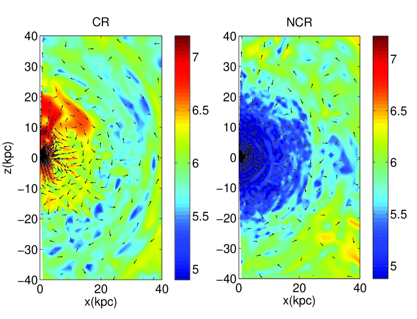
Figure 5.— Contour plot (in the $\phi=\pi$ plane) of $Log_{10}v$ (in cm s^-1) at 9 Gyr for CR (left) and NCR (right). Turbulent velocities $\gtrsim$ 100 km s^-1 are attained in inner 20 kpc for cosmic-ray driven convection (left). The turbulent velocities are significantly smaller in the absence of cosmic rays. Arrows show the $r-\theta$ projection of the velocity unit vector.

Figure 5 shows 2-D contour plots of turbulent velocity (absolute value of velocity) in the $\phi=\pi$ plane at 9 Gyr for CR and NCR. Velocities are similar for $r\gtrsim 30$ kpc where cosmic ray pressure is negligible and fluid motions are driven by the HBI. The maximum turbulent velocity in the HBI-dominated regions is $\sim 30$ km s^-1. Run CR shows much larger turbulent velocities ($\sim$ 100 km s^-1) for $r\lesssim 30$ kpc; note that the turbulent velocities induced by the ACRI are consistent with mixing length theory, with $L_{c}\sim 4\pi r^{2}\rho v_{c}^{3}$, where $L_{c}$ is the power carried by convection and $v_{c}$ is the resulting convective velocity. The large turbulent velocities in the presence of the ACRI are sufficient to prevent catastrophic cooling according to the models of Chandran & Rasera (2007). By contrast, the turbulent velocities are extremely small at $r\lesssim 30$ kpc for NCR because the plasma temperature gradient is wiped out by conduction before the HBI can drive any turbulence.

While the turbulent velocity vectors are roughly isotropic at $r\lesssim 30$ kpc for CR, they are aligned primarily perpendicular to the radial direction at large radii where the HBI dominates. This is consistent with the result that while the HBI saturates by reorienting magnetic field lines perpendicular to gravity (e.g., Parrish & Quataert, 2008), the ACRI drives roughly isotropic convection irrespective of the magnetic field geometry.

Figure 3 shows the time-averaged (from $t_{H}/2$ to $3t_{H}/4$) angle between the magnetic field vector and the radial direction as a function of radius for runs CR and NCR; the angle is defined with respect to the radial direction, such that it is $0^{0}$ for the initial split-monopole field. The average angle is similar for $r\gtrsim 30$ kpc, where the cosmic ray pressure is negligible, for both simulations. For run CR, radii $r\lesssim 30$ kpc are convectively stirred by the ACRI and the average angle between the magnetic field and the radial direction is $\approx 55^{0}$, close to the value expected for a uniform, random magnetic field unit vector ($\cos^{-1}1/2=60^{0}$). For both CR and NCR at 30 kpc $\lesssim r\lesssim 100$ kpc, the magnetic field is nearly perpendicular to the radial direction because of the HBI. The average angle between the magnetic field unit vector and the radial direction at these radii is $\approx 75^{0}$. For $r\gtrsim 100$ kpc and for $r\lesssim 20$ kpc in run NCR, the HBI is weak since thermal conduction wipes out the temperature gradient before the HBI can grow significantly; as a result, the field lines are not perpendicular to the radial direction.

Figure 6.— Time (from $t_{H}/2$ to $3t_{H}/4$) and angle averaged magnetic and kinetic energy densities (in erg cm^-3) as a function of radius for CR (solid line), CRM (long dashed line), and NCR (dotted line). The kinetic energy density is larger than the magnetic energy density in all cases. The initial magnetic energy density profile (short dashed line) is also shown for comparison. Run CRM, which includes a mean field, results in a much larger amplification of the magnetic energy as compared to CR.

Figure 6 shows angle and time averaged (from $t_{H}/2$ to $3t_{H}/4$) kinetic and magnetic energy profiles as a function of radius for runs CR, CRM, and NCR. Both the magnetic and kinetic energies are generally amplified, although to varying degrees. The kinetic energy is very effectively amplified at small radii by the action of the ACRI in run CR; the turbulent Mach number is $\sim 0.1$ (see also Fig. 5). The magnetic energy as a function of radius in CR is quite striking in that there is no magnetic energy enhancement at small radii: there is a slight bump in magnetic energy at 20 kpc but the final magnetic energy is smaller than the initial magnetic energy for $r\lesssim 3$ kpc. In turbulent dynamos one often finds the turbulent magnetic energy to be of the order of turbulent kinetic energy (e.g., Cho & Vishniac, 2000); this is clearly not the case for the run CR. Magnetic field amplification can, however, be subtle; e.g., in local shearing box simulations of the magnetorotational instability with no net magnetic flux, magnetic field amplification (and associated stress and turbulence) occurs only for Prandtl numbers exceeding unity (e.g., Fromang et al., 2007). We do not have explicit viscosity and resistivity and it is possible that the effective Prandtl number in our simulation is small, so that dissipation of the initially split monopolar field at the grid scale dominates over magnetic field enhancement by convective turbulence. To better understand this, we have done a simulation with cosmic rays with a net initial magnetic flux (run CRM), but with all other properties of the simulation the same. Figure 6 shows that in this case, the magnetic energy density is much larger in the inner regions as compared to CR, although the magnetic energy is still $\sim 100$ times smaller than the kinetic energy. In this case, the magnetic field strength in the center of the cluster is amplified to $\sim$ 0.1-1 $\mu$G by convective motions. The kinetic energy density profiles are almost identical for CR and CRM, indicating that the properties of the convection are not very different in the two cases, although the efficiency of magnetic field amplification differs dramatically.

At larger radii (30 kpc $\lesssim r\lesssim$ 100 kpc), the HBI causes amplification of the magnetic and kinetic energies in both CR and NCR. The magnetic energy is enhanced by a factor $\sim 100$ at $r\approx 60$ kpc. This level of field amplification – a factor of $\sim 10$, primarily of the $\theta$ and $\phi$ components – is what is required to reorient initially radial magnetic fields into fields that are perpendicular to the radial direction (as was seen in previous HBI and MTI simulations; Parrish & Quataert 2008; Parrish & Stone 2007; Sharma, Quataert, & Stone 2008). The kinetic energy is also enhanced at these radii because of turbulence driven by the HBI.

In order to study the numerical convergence of our fiducial run, we carried out an axisymmetric 2-D run analogous to CR – CR2D – and an axisymmetric run with double the resolution – CR2D-dbl (see Table 1); studying convergence directly with the 3D run CR would have been computationally prohibitive, requiring $\simeq 32$ times more cpu time. The results from runs CR2D and CR2D-dbl are nearly identical to each other; in particular, angle averaged plots such as those shown in Figures 2, 4, 3, and 6 are quite similar in the two cases. We have not included these 2-D results in every figure, but to illustrate the basic convergence result, Figure 3 shows that the average angle between the magnetic field unit vector and the radial direction is quite similar for CR2D and CR2D-dbl (which are both similar to the 3-D run CR). It is interesting to note that the 2-D runs differ from the 3-D run CR in one important respect: the amplification of the magnetic field at small radii is significantly larger in 2-D than in 3-D; the magnetic field energy density at small radii in the 2-D runs is comparable to the 3-D run with a net magnetic flux (CRM) in Figure 6. As mentioned earlier, the reason for the lack of significant magnetic field amplification in the run CR is not entirely clear.

3.2.2 Diffusion of a Passive Scalar

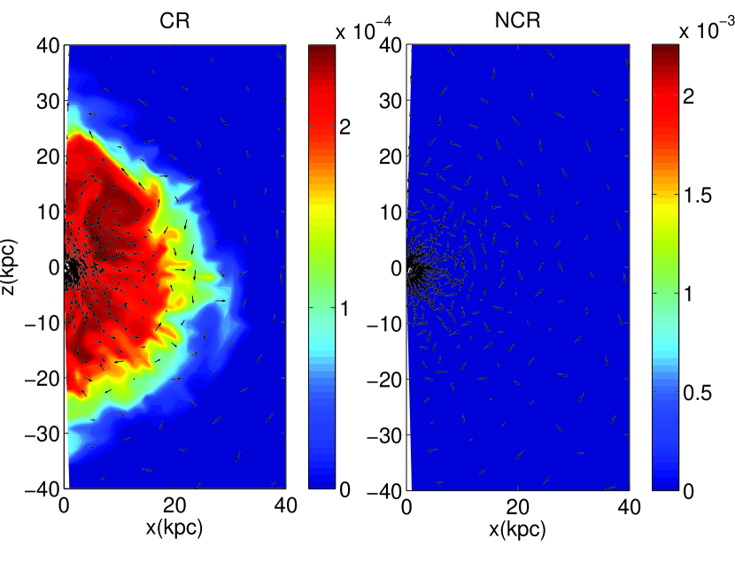
Figure 7.— Contour plot (at $\phi=\pi$) of the passive scalar density, $f$ (normalized to the initial maximum), at 9 Gyr for CR (left) and NCR (right). The passive scalar is initialized near the origin. Projection of magnetic field unit vector is over-plotted by arrows. While the passive scalar diffusion is negligible for NCR, turbulent mixing is efficient within 30 kpc for the cosmic-ray driven convection (left).

Figure 7 shows $f$, the passive scalar density, in the inner 40 kpc for CR and NCR at 9 Gyr, as well as the projection of the magnetic field unit vectors. The passive scalar density is initialized to be a large number ($f=10^{15}$) for $r<1.25$ kpc (corresponding to four radial zones) and is negligible ($f=10^{-15}$) for $r>1.25$ kpc. The goal of initializing a passive scalar is to study mixing due to turbulence. Observations of clusters reveal a metallicity distribution that is more spatially extended than the light distribution of the central galaxy. This may indicate turbulent transport of metals in clusters (e.g., Rebusco et al., 2006; Rasera & Chandran, 2008). As expected, run CR with large turbulent velocities at $r\lesssim 30$ kpc also results in efficient mixing. Mixing is negligible for NCR because the inner radii ($r\lesssim 30$ kpc) are isothermal and are thus not stirred by the HBI. For a direct comparison with observations, one must include a time dependent, spatially distributed source term in the passive scalar equation which represents metal enrichment due to Type Ia supernovae (e.g., Rebusco et al., 2005); this is beyond the scope of the present paper. Nonetheless, our results indicate that cosmic-ray driven convection is an efficient mechanism for mixing plasma in clusters of galaxies.

Figure 8.— Angle averaged passive scalar density ($Log_{10}f$; normalized to the initial maximum) as a function of radius for CR at 1/3, 1, 3, 9 Gyr (solid lines); the initial profile, shown by the dotted line, very close to the $y$ axis. Passive scalar density decreases as it spreads out with time. For comparison, the dashed line shows a Gaussian fit with a diffusion coefficient $D=10^{28}$ cm²s^-1 at 9 Gyr ($\sim\exp[-r^{2}/6Dt]$).

Figure 8 shows the angle averaged passive scalar density as a function of radius for run CR at 1/3, 1, 3, 9 Gyr. Also shown is a Gaussian fit (at 9 Gyr) with a diffusion coefficient of $10^{28}$ cm²s^-1. The passive scalar density at 9 Gyr is flatter than the Gaussian fit at $\lesssim$ 20 kpc, implying that diffusion due to convection driven by cosmic rays corresponds to an effective diffusion coefficient somewhat larger than $10^{28}$ cm²s^-1. Beyond $\sim 30$ kpc, the cosmic ray pressure is unimportant, and turbulence is driven by the HBI. This change in the source of the turbulence accounts for the rapid decline in the passive scalar density at large radii in Figure 8.

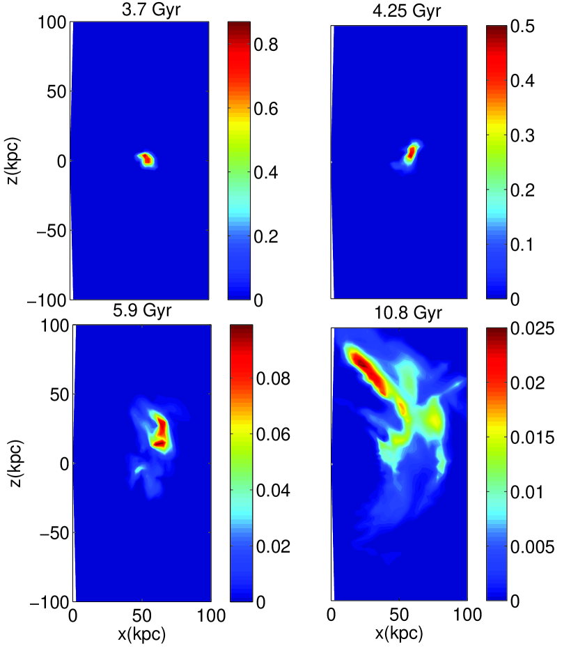
Figure 9.— Contour plot (at $\phi=\pi$) of the passive scalar density ($f$, normalized to the initial maximum) at 3.7, 4.25, 5.9, 10.8 Gyr for the run NCR. The passive scalar density is initialized in a small region (two grid points along $r,~{}\theta,~{}\phi$) centered at 53 kpc at 3.425 Gyr, and is negligible everywhere else. Turbulent mixing due to the HBI is faster in the $\theta$ direction compared to the radial direction.

To isolate just the mixing induced by turbulence driven by the HBI, we have taken run NCR at $t_{H}/4(=3.425$ Gyr) and initialized a passive scalar density peaked at $r\approx 53$ kpc, the radius where the temperature gradient is large and the HBI is active (see Fig. 2). The passive scalar is initialized to be $10^{15}$ at two grid points at $r=53$ kpc, $\theta=\pi/2$ and $\phi=\pi$, and negligible ($10^{-15}$) elsewhere. Figure 9 shows $\phi=\pi$ snapshots of the passive scalar density at later times. The passive scalar diffuses more rapidly in the $\theta$ direction. This is because the turbulent velocities due to the HBI are larger in the direction perpendicular to gravity than they are in the radial direction (just as the magnetic field components perpendicular to gravity are preferentially amplified). To estimate the diffusion coefficient in the $r$ and $\theta$ directions, we compare how much the passive scalar has spread in the two directions; the full width at half maximum (FWHM) for $f$ along $r$ and $\theta$ at 9 Gyr is $\approx 10$, 40 kpc, respectively. For comparison, the FWHM at 9 Gyr for $f$ for run CR shown in Fig. 8 is $\approx 60$ kpc. Thus the diffusion coefficient due to the HBI alone is $\sim 2$ (perpendicular to gravity) and $\sim 50$ (parallel to gravity) times smaller than the diffusion coefficient due to the ACRI in run CR. Although these precise numerical values likely depend on the detailed parameters of our simulations, the fact that the HBI primarily induces turbulence and mixing in the plane perpendicular to gravity is a generic result.

3.2.3 Heat Flux modified by the HBI and ACRI

Many 1-D models of clusters parameterize thermal conduction by its ratio to the Spitzer value (Zakamska & Narayan, 2003; Chandran & Rasera, 2007; Guo & Oh, 2008). However, our simulations show that, because of plasma instabilities that operate in clusters (e.g., HBI and ACRI), a reduction of the conductivity by a fixed factor is not applicable (see also Parrish & Stone 2007; Parrish & Quataert 2008; Sharma, Quataert, & Stone 2008). At large radii in cluster cores, where the cosmic ray pressure is negligible, the HBI can orient field lines perpendicular to the radial direction, but at small radii where cosmic rays can be significant, the magnetic field may be significantly more radial. For example, for run CR the average angle of the magnetic field relative to the radial direction for $r\lesssim 30$ kpc is $\sim 55^{0}$ (see Fig. 3), corresponding (roughly) to a reduction factor of $(\mbox{\boldmath$\hat{b}\cdot\hat{r}$})^{2}\approx 1/3$. For 30 kpc $\lesssim r\lesssim 100$ kpc, however, the turbulence is dominated by the HBI, and the average angle between the magnetic field and the radial direction is $\approx 75^{0}$, corresponding to a reduction factor of $\approx 0.07$.

An even more subtle result is that the HBI can change the background temperature gradient by forming thermal barriers (see Fig. 2), which will be absent with isotropic conduction. For example, the temperature gradient at 30 kpc $\lesssim r\lesssim$ 100 kpc for CR and NCR at late times is $\approx 3$ times larger than the initial temperature gradient. Thus, the HBI not only reduces the conductive heating by a factor of $(\mbox{\boldmath$\hat{b}\cdot\hat{r}$})^{2}\approx 0.07$, it also increases it by making the temperature gradient larger by a factor $\approx 3$. Approximating the conductivity of a magnetized plasma by a constant factor with respect to the Spitzer value misses all of this interesting dynamics. Whether this is important in real clusters with radiative cooling and various sources of heating remains to be seen.

3.2.4 Runs with larger $D_{\parallel}$ (CR28 & CR29)

We have also carried out 2-D simulations with larger cosmic ray diffusion coefficients ($D_{\parallel}$), since the value of the cosmic ray diffusion coefficient is poorly constrained (see §2.2). Run CR28 uses $D_{\parallel}=10^{28}$ cm² s^-1, the cosmic ray diffusion coefficient estimated for GeV cosmic rays in the Galaxy. Run CR29 uses $D_{\parallel}=10^{29}$ cm² s^-1. All other parameters and initial conditions are same as the fiducial run. Since we are comparing these 2-D simulations with CR, which is a 3-D simulation, we have verified that the run CR2D gives results similar to the 3-D results presented here; in particular, the profiles for $p_{\rm cr}/\rho^{\gamma_{\rm cr}}$ and $p_{\rm cr}/p$ are identical to the profiles for CR shown in Figure 4.

Figure 10.— Angle averaged cosmic ray entropy (upper panel; arbitrary normalization) and the ratio of cosmic ray to plasma pressure (lower panel) as a function of radius for the runs CR28 (left) and CR29 (right), which use a fixed cosmic ray diffusion coefficients of $D_{\parallel}=10^{28}$ and $10^{29}$ cm²s^-1, respectively. The solid lines show profiles at 1/3, 1, 3, 9 Gyr, with the entropy and pressure ratio increasing in time; the initial profiles are shown with dotted lines. Profiles for CR28 look similar to profiles for CR in Figure 4. The profiles for CR29 are different in that $p_{\rm cr}/\rho^{\gamma_{\rm cr}}$ and $p_{\rm cr}/p$ increase towards a maximum at the intermediate radii; this is because the cosmic-rays are no longer adiabatic for large $D_{\parallel}$.

Figure 10 shows the angle averaged cosmic ray entropy ($p_{\rm cr}/\rho^{\gamma_{\rm cr}}$) and the ratio of the cosmic ray pressure to the plasma pressure ($p_{\rm cr}/p$) as a function of radius for CR28 and CR29. The profiles for CR28 and CR (see Fig. 4) look similar; cosmic ray entropy and pressure are slightly more radially spread out for CR28. The profiles for CR29 are quite different. The entropy and pressure ratio profiles have a peak at $\sim 20$ kpc; this is the radius beyond which the cosmic ray diffusion time is longer than the buoyancy timescale (see Fig. 1). The ratio $p_{\rm cr}/p$ is smaller in CR29 as cosmic rays are spread out over a larger volume by diffusion. The cosmic ray entropy increases outwards for $r\lesssim 20$ kpc since cosmic ray diffusion, and not convection driven by cosmic rays, dominates the outward cosmic ray transport. This is different from CR and CR28 where cosmic ray diffusion is sub-dominant. Even in CR29, cosmic rays are effectively adiabatic for $r\gtrsim 20$ kpc; cosmic-ray driven convection is absent at these radii, however, because the cosmic ray pressure is not large enough to drive the ACRI (see Fig. 10). At smaller radii, the cosmic rays are nearly isobaric because of rapid diffusion, and the system is formally unstable to the CR mediated version of the MTI (eq. [17]). However, because the field lines are nearly radial at these radii, the growth-rate of the CRMTI is quite slow and we do not see any indications that it develops in our simulations.

To explicitly study the possibility of the ACRI setting in at larger radii in the cluster core, we carried out a simulation with the cosmic ray source term (eq. [20]) three times larger than in run CR29. This larger source term increases the CR pressure at large radii, and at late times $p_{\rm cr}/p$ is large enough to drive the ACRI. The turbulent velocities are $\sim 100$ km s^-1 at $r\sim 20-30$ kpc, where the cosmic rays are effectively adiabatic in spite of the large $D_{\parallel}$. Thus, even in the presence of rapid cosmic ray diffusion, the ACRI can set in at large radii where the cosmic rays are adiabatic, provided the cosmic ray pressure is sufficiently large; this may naturally occur in the vicinity of cosmic-ray filled buoyant bubbles. More generally, our results demonstrate that so long as $D_{\parallel}\lesssim 1-3\times 10^{28}$, cm² s^-1, cosmic rays will behave effectively adiabatically throughout the cluster core and bulk transport by convection and other mechanisms will dominate the diffusive transport.

3.2.5 Runs with Cosmic ray Sources at the Poles (CR30 & CR30-ad)

It is very unlikely that cosmic rays in clusters are injected spherically symmetrically. Instead, the injection likely occurs preferentially in the polar direction. To study the resulting physics in this case, we carried out 3-D simulations in which the cosmic ray source term is applied only within $30^{0}$ of the pole: CR30 and CR30-ad. Except for this difference all parameters for run CR30 are the same as run CR. Run CR30-ad differs from CR30 in that the plasma is adiabatic, i.e., thermal conduction is not included. One of the aims of these simulations is to show the dramatic differences that result from including anisotropic thermal conduction (relative to a more typical adiabatic simulation). Cluster plasmas are observed to be stable to adiabatic convection because the entropy increases outwards (e.g., Piffaretti et al., 2005). However, convection in an anisotropically conducting plasma depends on the temperature gradient, and not the entropy gradient, and the system is unstable independent of the sign of the temperature gradient. This makes it much easier to mix a thermally conducting plasma than an adiabatic plasma. In clusters, this implies that turbulence produced by external means, e.g., the ACRI, wakes due to galaxy clusters, etc., may be an effective way of mixing the thermal plasma.

Figure 11.— Contour plots within 40 kpc, in the $\phi=\pi$ plane, of $Log_{10}(p_{\rm cr}/p)$ for runs CR30 (top) and CR30-ad (bottom) at $t=$ 1/3, 1, 3, and 6 Gyr (from left to right). The ratio $p_{\rm cr}/p$ is not shown if it is smaller than $10^{-4}$. The adiabatic plasma in CR30-ad (bottom) artificially suppresses the angular and radial mixing of the relativistic and thermal plasma that is present in the simulations with anisotropic thermal conduction (CR30; top). For movies corresponding to this figure, see: http://astro.berkeley.edu/$\sim$psharma/clustermovie.html.

Figure 11 shows contour plots ($\phi=\pi$ snapshot) of the ratio of cosmic ray pressure to plasma pressure ($p_{\rm cr}/p$) at 1/3, 1, 3, 6 Gyr, for CR30 and CR30-ad. For CR30, the cosmic rays become unstable to the ACRI in the polar region. The resulting turbulence is able to convectively mix the plasma, not only in the unstable radial direction, but also in the marginally stable $\theta$ direction. Instead of cosmic rays being confined only to the $\theta=30^{0}$ cone, convection effectively mixes plasma in both the radial and angular directions. In addition, at radii beyond 20 kpc where the temperature gradient is appreciable (see Fig. 2), the HBI mixes material primarily in the $\theta$ direction, as seen by the $\theta-$oriented fingers at late times in Figure 11. For CR30, $p_{\rm cr}/p\approx 0.02$ at 3 Gyr in the equatorial region for $r\lesssim 10-20$ kpc. Although cosmic rays are still dominant near the pole, convection brings a non-negligible amount cosmic rays into the equatorial region. In comparison, there is no sign of convective overshoot in CR30-ad because convective motions in the thermal plasma near the equator are strongly stabilized by a large positive plasma entropy gradient. The polar cosmic ray dominated plasma does expand somewhat in both $r$ and $\theta$ as it becomes over-pressured. However, the value of $p_{\rm cr}/p$ at 3 Gyr is $\lesssim 10^{-4}$ everywhere in the equatorial plane for CR30-ad.

4. Summary & Astrophysical Implications

The X-ray emitting plasma in clusters of galaxies is hot ($T\sim 1-10$ keV) and dilute ($n\sim 0.001-0.5$ cm^-3), so that the transport of heat and momentum along magnetic field lines can be energetically and dynamically important. In addition, jets launched by a central AGN produce relativistic plasma (cosmic rays), which are observed in part as bubbles of radio emission associated with deficits of thermal X-ray emission (X-ray cavities; e.g., Bîrzan et al. 2004). In this paper we have studied the transport properties of an ICM composed of cosmic rays and thermal plasma. We have argued that cosmic ray diffusion is likely to be slow because of scattering by self-generated Alfvén waves (§2.2); as a result, the cosmic rays are adiabatic on moderately large length scales $\gtrsim$ 1-10 kpc. More concretely, cosmic rays are adiabatic on the scale of cluster cores, so long as their parallel diffusion coefficient satisfies $D_{\parallel}\lesssim 10^{29}$ cm²s^-1.

It is now well established that anisotropic conduction and anisotropic cosmic ray diffusion can dramatically modify buoyancy instabilities in low collisionality systems, producing qualitatively new instabilities such as the MTI, HBI, and their cosmic ray counterparts (e.g., Balbus, 2000; Chandran & Dennis, 2006; Parrish & Stone, 2007; Quataert, 2008; Parrish & Quataert, 2008). Nonlinear studies of these instabilities (including those in this paper) have demonstrated that they saturate by approaching a state of marginal stability to linear perturbations, just as in hydrodynamic convection. However, in a magnetized plasma, there is an additional degree of freedom that is not present in hydrodynamic convection, namely the local direction of the magnetic field. The primary mechanism by which these diffusive buoyancy instabilities saturate is by rearranging the magnetic field lines, so that the linear growth rate becomes extremely small (see Fig. 3). This is different from entropy gradient driven convection in adiabatic fluids, which saturates by producing convection that wipes out strong entropy gradients. Even nonlinearly, most of the energy flux in systems unstable to the MTI and HBI is transported by thermal conduction, rather than convection. Moreover, the saturation of these instabilities is quasilinear in the sense that the saturated magnetic energy is proportional to the initial magnetic field energy (Sharma, Quataert, & Stone, 2008).

In this paper we have shown analytically and through numerical simulations that when cosmic rays have appreciable pressure, $p_{\rm cr}/p\gtrsim 0.25$, and an outwardly decreasing entropy ($p_{\rm cr}/\rho^{\gamma_{\rm cr}}$), they can drive strong convection and mixing in clusters of galaxies. This adiabatic cosmic ray instability (ACRI) in the central regions of clusters of galaxies is a cosmic ray analogue of hydrodynamic convection familiar in the context of stars and planets. In particular, the nonlinear saturation of adiabatic cosmic ray convection is similar to that of hydrodynamic convection, and thus quite different from the saturation of the MTI and HBI. Our simulations of cluster cores also provide insight into the global saturation of the HBI at radii in clusters where the cosmic ray pressure is negligible ($\sim 30-100$ kpc in our models), and thus where the only convective instability is that driven by the background conductive heat flux. More specifically, the primary results of this paper include:

• If the cosmic ray entropy decreases outwards and if $p_{\rm cr}/p\gtrsim 0.25$, convection driven by the ACRI sets in. In the saturated state, the cosmic ray entropy profile becomes nearly constant in the region with significant cosmic ray pressure (Fig. 4). The resulting turbulent velocities are consistent with mixing length theory, with $v_{c}\sim 100(L_{c}/10^{43}\,{\rm erg\,s^{-1}})^{1/3}\,(n/0.1\,{\rm cm^{-3}})^{-1/3}(r_{0}/20{\rm kpc})^{-2/3}$ km s^-1 where $L_{c}$ is the total power supplied to cosmic rays and $r_{0}$ is the pressure height scale of cosmic rays. The ACRI generates turbulent motions more effectively in cluster cores than the HBI alone.

• The ACRI drives roughly isotropic convection with the average angle between the field lines and the radial direction $\sim 55^{0}$; by contrast, the HBI generates magnetic field lines that are primarily in the $\theta$ and $\phi$ directions (Fig. 3), shutting off the radial conduction of heat. The effective radial conductivity of a cluster plasma thus depends sensitively on which of these instabilities operates at a given location, and may not be adequately approximated as a fixed fraction of the Spitzer value throughout the cluster.

• We have quantified the mixing of a passive scalar by the ACRI and HBI: the ACRI produces roughly isotropic mixing with a turbulent diffusion coefficient $D\gtrsim 10^{28}$ cm²s^-1 (Fig. 7); mixing length theory predicts that $D\propto v_{c}\propto L_{c}^{1/3}$. At larger radii, only the HBI operates and the mixing is primarily in the $\theta$ and $\phi$ directions, rather than in the radial direction (Fig. 9). Both the ACRI and the HBI may contribute to mixing metals in clusters by redistributing, in both radius and angle, metals produced by Type 1a supernovae. Some observations of metallicity gradients in clusters have inferred mixing at levels comparable to those found here (e.g., Rebusco et al., 2006).

• It is considerably easier to mix thermal plasma in the presence of anisotropic thermal conduction, since the plasma is formally always buoyantly unstable and thus already prone to mixing! By contrast, treating the plasma as adiabatic (i.e., ignoring thermal conduction) results in an artificially stabilizing entropy gradient in cluster plasmas. As a concrete example of these effects, we have demonstrated that cosmic rays initially injected into the polar regions can be partially mixed to the equator by convective overshooting in the ACRI and HBI unstable regions (Fig. 11); this effect is largely absent in simulations that treat the plasma as adiabatic. If wave heating due to cosmic ray streaming or heating due to Coulomb interactions is important in clusters (e.g., Guo & Oh 2008), a mechanism similar to that described here may be crucial in redistributing cosmic rays throughout the cluster volume. More generally, to study the mixing produced by external sources of turbulence such as galactic wakes or cosmic-ray filled bubbles, we suspect that anisotropic thermal conduction must be accounted for, so that the buoyant response of the thermal plasma is correctly represented.

Having summarized our primary results, we now describe several caveats and directions for future research. First, to generate the ACRI, we have injected cosmic rays using a subsonic source term at small radii. In reality a significant fraction of the cosmic rays produced by an AGN are expected to be produced in a supersonic jet shocking against the ICM. The spatial distribution of cosmic rays produced by jets is poorly understood. The intuition drawn from our simulations should apply as long the source of cosmic rays ultimately produces a centrally concentrated bubble of relativistic plasma that expands subsonically.

Our calculations intentionally do not include plasma cooling. Instead of trying to solve the cooling flow problem, our goal has been to study the basic physics of buoyancy instabilities in the combined relativistic + thermal plasma, implicitly assuming that some heating process is preventing catastrophic cooling of the plasma. Our calculations also do not include anisotropic ion viscosity which is $\approx 40$ times smaller than electron thermal conductivity. Finally, we do not treat the effects of cosmic ray streaming with respect to the thermal plasma from first principles, although our choice of the cosmic ray diffusion coefficient qualitatively accounts for limits on cosmic ray streaming produced by self-excited Alfvén waves (see §2.2). In future work, we intend to include all of the above effects, which will provide a more quantitative model of plasma in cluster cores.

Finally, we note that in a full cosmological context, galaxy clusters will contain a large number of galaxies and other dark matter substructure. The motion of such bound objects through the ICM will reorient the magnetic field and generate downstream turbulence. The interplay between this turbulence and that generated by the instabilities studied in this paper is worth investigating in detail in future work. This interaction may create a magnetic dynamo in the ICM that is more effective than that produced by the HBI alone: galaxies moving through the ICM will comb out the magnetic field lines in the radial direction, while the HBI will amplify the field and generate a strong perpendicular magnetic field component from the seed radial field created by galactic wakes.

Appendix A Numerical Tests

Figure 12.— Profiles for different fluid variables for the shock tube test: initial profiles (solid line) and profiles at $t=4.4\times 10^{-4}$ (points). While the shock is resolved by 4 points, contact discontinuity requires more grid points to be resolved (this is a feature of all methods that do not solve the full Riemann problem).

A.1. Cosmic ray shock tube

We have tested the adiabatic implementation of cosmic rays with a 1-D shock tube problem discussed in Pfrommer et al. (2006) and in Rasera & Chandran (2008). Like Rasera & Chandran (2008), we also use 1024 grid points. Thermal conduction and cosmic ray diffusion are absent for this test problem. The left ($1<x<1.5$) and right ($1.5\leq x<2$) states are given by ($\rho_{L}$, $v_{L}$, $p_{L}$, $p_{crL}$) = (1, 0, $6.7\times 10^{4}$, $1.3\times 10^{5}$) and ($\rho_{R}$, $v_{R}$, $p_{R}$, $p_{crR}$) = (0.2, 0, $2.4\times 10^{2}$, $2.4\times 10^{2}$), respectively. Figure 12 shows profiles at $t=0$ (solid line) and at $t=4.4\times 10^{-4}$ (shorter than the crossing time; points). The profiles match very well with the analytic result and with Fig. 3 of Rasera & Chandran (2008). In addition we also test advection of a passive scalar density governed by equation (21). The passive scalar density shows a discontinuity at the location of the contact discontinuity; volume integrated $f$ is not conserved but volume integrated $\rho f$ is.

References

- Allen et al. (2006) Allen, S. W., Dunn, R. J. H., Fabian, A. C., Taylor, G. B., & Reynolds, C. S. 2006, MNRAS, 372, 21
- Balbus (2000) Balbus, S. A. 2000, ApJ, 534, 420
- Berezinskii et al. (1990) Berezinskii, V. S., Bulanov, S. V., Dogiel, V. A., & Ptuskin, V. S., Astrophysics of Cosmic Rays, Amsterdam:North-Holland, 1990, Ed. Ginzburg, V. L.
- Bertschinger & Meiksin (1986) Bertschinger, E. & Meiksin, A. 1986, ApJ, 306, L1
- Binney & Tabor (1995) Binney, J. & Tabor, G. 1995, MNRAS, 276, 663
- Bîrzan et al. (2004) Bîrzan, L., Rafferty, D. A., McNamara, B. R., Wise, M. W., & Nulsen, P. E. J. 2004, ApJ, 607, 800
- Braginskii (1965) Braginskii, S. I., Reviews of Plasma Physics, Vol. 1, Consultants Bureau, 1965
- Chandran & Dennis (2006) Chandran, B. D. G. & Dennis, T. J. 2006, ApJ, 642, 140
- Chandran & Rasera (2007) Chandran, B. D. G. & Rasera, Y. 2007, ApJ, 671, 1413
- Cho & Vishniac (2000) Cho, J. & Vishniac, E. T. 2000, ApJ, 538, 217
- Churazov et al. (2008) Churazov, E., Forman, W., Vikhlinin, A., Tremaine, S., Gerhard, O., & Jones, C. 2008, MNRAS, 388, 1062
- Ciotti & Ostriker (2001) Ciotti, L. & Ostriker, J. P. 2001, ApJ, 2001, 551, 131
- Conroy & Ostriker (2008) Conroy, C. & Ostriker, J. P. 2008, ApJ, 681, 151
- Dennis & Chandran (2008) Dennis, T. & Chandran, B. D. G. 2009, ApJ, 690, 566
- Drury & Völk (1981) Drury, L. & Völk, H. 1981, ApJ, 248, 344
- Eilek (2003) Eilek, J. A. 2003, Proc. of The Riddle of Cooling Flows in Galaxies and Clusters of Galaxies, E13, Ed. T. H. Reipeich, J. C. Kempner, & N. Soker
- Engelmann et al. (1990) Engelmann, J. J. et al. 1990, A&A, 233, 96
- Fabian (1994) Fabian, A. C. 1994, ARA&A, 32, 277
- Fromang et al. (2007) Fromang, S., Papaloizou, J., Lesur, G., & Heinemann, T. 2007, A&A, 476, 1123
- Govoni & Feretti (2004) Govoni, F. & Luigina, F. 2004, Int. J. Mod. Phys. D, 13, 1549
- Guo & Oh (2008) Guo, F. & Oh, S. P. 2008, MNRAS, 384, 251
- Hayes et al. (2006) Hayes, J. C. et al. 2006, ApJS, 165
- Johnstone et al. (2002) Johnstone, R. M., Allen, S. W., Fabian, A. C., & Sanders, J. S. 2002, MNRAS, 336, 299
- Kelson et al. (2002) Kelson, D. D. et al. 2002, ApJ, 576, 720
- Kulsrud & Pearce (1969) Kulsrud, R. M. & Pearce, W. P. 1969, ApJ, 156, 445
- Kulsrud (2005) Kulsrud, R. M., Plasma Physics for Astrophysics 2005, Princeton Univ. Press
- Loewenstein, Zweibel, & Begelman (1991) Loewenstein, M., Zweibel, E. G., & Begelman, M. C. 1991, ApJ, 377, 392
- Navarro, Frenk, & White (1997) Navarro, J. F., Frenk, C. S., & White, S. D. M. 1997, ApJ, 490, 493
- Parrish & Stone (2007) Parrish, I. J. & Stone, J. M. 2007, ApJ, 664, 135
- Parrish & Quataert (2008) Parrish, I. J. & Quataert, E. 2008, ApJ, 677, L9
- Parrish, Stone, & Lemaster (2008) Parrish, I. J., Stone, J. M., & Lemaster, M. N. 2008, ApJ, 688, 905
- Peterson et al. (2003) Peterson, J. R. et al. 2003, ApJ, 590, 207
- Pfrommer & Enßlin (2004) Pfrommer, C. & Enßlin, T. A. 2004, A&A, 413, 17
- Pfrommer et al. (2006) Pfrommer, C. et al. 2006, MNRAS, 367, 113
- Piffaretti et al. (2005) Piffaretti, R. et al. 2005, A&A, 433, 101
- Quataert (2008) Quataert, E. 2008, ApJ, 673, 758
- Rasera & Chandran (2008) Rasera, Y. & Chandran, B. 2008, ApJ, 685, 105
- Rasera et al. (2008) Rasera, Y., Srivastava, K., & Chandran, B. 2008, ApJ, 689, 825
- Rebusco et al. (2005) Rebusco, P. Churazov, E., Böhringer, H., & Forman, W. 2005, MNRAS, 359, 1041
- Rebusco et al. (2006) Rebusco, P., Churazov, E., Böhringer, H., & Forman, W. 2006, MNRAS, 372, 1840
- Reynolds et al. (2005) Reynolds, C. S., McKernan, B., Fabian, A. C., Stone, J. M., & Vernaleo, J. C. 2005, MNRAS, 357, 242
- Rosner & Tucker (1989) Rosner, R. & Tucker, W. H. 1989, ApJ, 338, 761
- Schwarzschild (1958) Schwarzschild, M., Structure and Evolution of Stars, Princeton University Press, 1958
- Sharma & Hammett (2007) Sharma, P. & Hammett, G. W. 2007, J. Comp. Phys., 227, 123
- Sharma, Quataert, & Stone (2008) Sharma, P., Quataert, E., & Stone, J. M. 2008, MNRAS, 389, 1815
- Stone & Norman (1992a) Stone, J. M. & Norman, M. L. 1992, ApJS, 80, 753
- Stone & Norman (1992b) Stone, J. M. & Norman, M. L. 1992, ApJS, 80, 791
- Vernaleo & Reynolds (2006) Vernaleo, J. C. & Reynolds, C. S. 2006, ApJ, 645, 83
- Zakamska & Narayan (2003) Zakamska, N. & Narayan, R. 2003, ApJ, 582, 162