Average-case analysis of perfect sorting by reversals

Abstract

A sequence of reversals that takes a signed permutation to the identity is perfect if at no step a common interval is broken. Determining a parsimonious perfect sequence of reversals that sorts a signed permutation is NP-hard. Here we show that, despite this worst-case analysis, with probability one, sorting can be done in polynomial time. Further, we find asymptotic expressions for the average length and number of reversals in commuting permutations, an interesting sub-class of signed permutations.

1 Introduction

The sorting of signed permutations by reversals is a simple combinatorial problem with a direct application in genome arrangement studies. Different sorting scenarios provide estimates for evolutionary distance and can help explain the differences in gene orders between two species (see [9] for example). Initially, the shortest sequences (parsimonious) of reversals were sought, and polynomial time algorithms to find such sequences were described ([13, 8, 18]). Recently, biologically motivated refinements have been considered, specifically accounting for groups of genes that are co-localized with the different homologous genes (genes having a single common ancestor) in the genomes of different species. These groups are likely together in the common ancestral genome, and were not disrupted during evolution, hence, we expect them to appear together at every step of the evolution. In terms of our combinatorial model, a group of co-localized genes is modeled by a common interval, that is, a collection of sequential numbers that are not broken by any reversal move. This constraint leads us back to the basic algorithmic problem:

What is the smallest number of reversals required to sort a signed permutation into the identity permutation without breaking any (subset of) common interval?

These scenarios are called perfect [11]. Because of the additional constraint, it is possible that the smallest perfect sorting scenario is longer that the smallest scenario.

Already it is known that this refined problem is NP-hard [11]. However, several authors have given sub-instances which can be solved in polynomial time [3, 4, 10], and fixed parameter tractable algorithms exist [4, 5]. For example, commuting permutations are the sub-class with the striking property that the property of a scenario being perfect is preserved even when the sequence of reversals is reordered. Examples of commuting scenarios arise in the study of mammals. All of the known sub-problems can be expressed in terms of the “strong interval tree” associated to a permutation, and we focus our attention on the structure of this tree.

Recently, several works have investigated expected properties of combinatorial objects related to genomic distance computation, such as the breakpoint graph  [20, 21, 19, 17]. We explore this route here, but focusing on the strong interval tree, to conduct an average case analysis of perfect sorting by reversals. First, in Section 3, we prove that for large enough $n$, with probability $1$, computing a perfect reversal sorting scenario for signed permutations can be done in time polynomial in $n$, despite the fact that this is NP-hard. Secondly, in Section 4, we show that in parsimonious perfect scenarios for commuting permutations of length $n$, the average number of reversals is asymptotically $1.2n$, and the average length of a reversal is $1.02\sqrt{n}$.

2 Preliminaries

We first summarize the combinatorial and algorithmic frameworks for perfect sorting by reversals. For a more detailed treatment, we refer to [4].

Permutations, reversals, common intervals and perfect scenarios.

A signed permutation on $[n]$ is a permutation on the set of integers $[n]=\{1,2,\ldots,n\}$ in which each element has a sign, positive or negative. Negative integers are represented by placing a bar over them. We denote by $Id_{n}$ (resp. $\overline{Id_{n}}$) the identity (resp. reversed identity) permutation, $(1\ 2\ldots n)$ (resp. $(\overline{n}\ldots\overline{2}\ \overline{1})$). When the number $n$ of elements is clear from the context, we will simply write $Id$ or $\overline{Id}$.

An interval $I$ of a signed permutation $\sigma$ on $[n]$ is a segment of adjacent elements of $\sigma$. The content of $I$ is the subset of $I$ defined by the absolute values of the elements of $I$. Given $\sigma$, an interval is defined by its content and from now, when the context is unambiguous, we identify an interval with its content.

The reversal of an interval of a signed permutation reverses the order of the elements of the interval, while changing their signs. If $\sigma$ is a permutation, we denote by $\overline{\sigma}$ the permutation obtained by reversing the complete permutation $\sigma$. A scenario for $\sigma$ is a sequence of reversals that transforms $\sigma$ into $Id_{n}$ or $\overline{Id_{n}}$. The length of such a scenario is the number of reversals it contains. The length of a reversal is the number of elements in the interval that is reversed.

Two distinct intervals $I$ and $J$ commute if their contents trivially intersect, that is either $I\subset J$, or $J\subset I$, or $I\cap J=\emptyset$. If intervals $I$ and $J$ do not commute, they overlap. A common interval of a permutation $\sigma$ on $[n]$ is a subset of $[n]$ that is an interval in both $\sigma$ and the identity permutation $Id_{n}$. The singletons and the set $\{1,2,\ldots,n\}$ are always common intervals called trivial common intervals.

A scenario $S$ for $\sigma$ is called a perfect scenario if every reversal of $S$ commutes with every common interval of $\sigma$. A perfect scenario of minimal length is called a parsimonious perfect scenario.

A permutation $\sigma$ is said to be commuting if, there exists a perfect scenario for $\sigma$ such that for every pair of reversals of this scenario, the corresponding intervals commute. In such a case, this property holds for every perfect scenario for $\sigma$ [4].

The strong interval tree.

A common interval $I$ of a permutation $\sigma$ is a strong interval of $\sigma$ if it commutes with every other common interval of $\sigma$.

The inclusion order of the set of strong intervals defines an $n$-leaf tree, denoted by $T_{\mathcal{S}}(\sigma)$, whose leaves are the singletons, and whose root is the interval containing all elements of the permutation. The strong interval tree of $\sigma$ can be computed in linear time and space (see [7] for example). We call the tree $T_{\mathcal{S}}(\sigma)$ the strong interval tree of $\sigma$, and we identify a vertex of $T_{\mathcal{S}}(\sigma)$ with the strong interval it represents. In a more combinatorial context, this tree is also called substitution decomposition tree [1]. If $\sigma$ is a signed permutation, the sign of every element of $\sigma$ is given to the corresponding leaves in $T_{\mathcal{S}}(\sigma)$.

Let $I$ be a strong interval of $\sigma$ and ${\cal I}=(I_{1},\dots,I_{k})$ the unique partition of the elements of $I$ into maximal strong intervals, from left to right. The quotient permutation of $I$, denoted $\sigma_{I}$, is defined as follows: $\sigma_{I}(i)$ is smaller than $\sigma_{I}(j)$ in $\sigma_{I}$ if any element of $I_{i}$ is smaller (in absolute value if $\sigma$ is a signed permutation) than any element of $I_{j}$. The vertex $I$, or equivalently the strong interval $I$ of $\sigma$, is either: increasing linear, if $\sigma_{I}$ is the identity permutation, or decreasing linear, if $\sigma_{I}$ is the reversed identity permutation, or prime, otherwise. For exposition purposes we consider that an increasing vertex is positive and a decreasing vertex is negative. The strong interval tree as computed in the algorithm of [7] contains the nature -increasing/decreasing linear or prime- of each vertex. It can be adapted to compute also in linear time the quotient permutation associated to each strong interval. (See Fig. 1 for an example.)

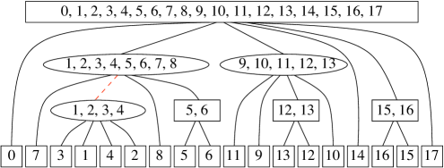
Figure 1: The strong interval tree $T_{\mathcal{S}}(\sigma)$ of the permutation $\sigma=(1~{}\bar{8}~{}4~{}2~{}\bar{5}~{}3~{}9~{}\bar{6}~{}7~{}12~{}10~{}\bar{14}~{}13~{}\bar{11}~{}15~{}\bar{17}~{}16~{}18)$. Prime and linear vertices are distinguished by their shape. There are three non-trivial linear vertices, the rectangular vertices, and three prime vertices, the round vertices. The root and the vertex $\{6,7\}$ are increasing linear vertices, while the linear vertices $\{16,17\}$ and $\{13,14\}$ are decreasing.

For a vertex $I$ of $T_{S}(\sigma)$, we denote by $L(I)$ the set of elements of $\sigma$ that label leaves of the subtree of $T_{S}(\sigma)$ rooted at $I$.

The strong interval tree as a guide for perfect sorting by reversals.

We describe now important properties, related to the strong interval tree, of the algorithm described in [4] for perfect sorting by reversals a signed permutation. Let $\sigma$ be a signed permutation of size $n$ and $T_{S}(\sigma)$ its strong interval tree, having $m$ internal vertices, called $I_{1},\ldots,I_{m}$, including $p$ prime vertices:

Theorem 1.

[4]

1. The algorithm described in [4] can compute a parsimonious perfect scenario for $\sigma$ in worst-case time $O(2^{p}n\sqrt{n\log(n)})$.

2. $\sigma$ is a commuting permutation if and only if $p=0$.

3. If $\sigma$ is a commuting permutation, then every perfect scenario has for reversals set the set $\{L(I_{j})|I_{j}\text{ has a sign different from its parent in $T_{\mathcal{S}}(\sigma)$}\}$

Remark 1.

The strong interval tree of an unsigned permutation is equivalent to the modular decomposition tree of the corresponding labeled permutation graph (see [4] for example). Also commuting permutations have been investigated, in connection with permutation patterns, under the name of separable permutations [14].

3 On the number of prime vertices

Motivated by the average-time complexity of the algorithm described in [4] for computing a parsimonious perfect scenario, we first investigate the average shape of a strong interval tree of a permutation of size $n$. Such a tree is characterized by the shape of the tree along with the quotient permutations labeling internal vertices. For prime vertices, those quotient permutations correspond to simple permutations as defined in [2]. We first concentrate on enumerative results on simple permutations. Next, we derive from them enumerative consequences on the number of permutations whose strong interval tree has a given shape. Exhibiting a family of shapes with only one prime vertex, we can prove that nearly all permutations have a strong interval tree of this special shape.

3.1 Combinatorial preliminaries: strong interval trees and simple permutations

Let $T_{\mathcal{S}}(\sigma)$ be the strong interval tree of a permutation $\sigma$ of length $n$. From a combinatorial point of view it is simply a plane tree (the children of a vertex are totally ordered) with $n$ leaves and its internal vertices labeled by their quotient permutation: an internal vertex having $k$ children can be labeled either by the permutation $(1\ 2\ \ldots\ k)$ (increasing linear vertex), the permutation $(k\ k-1\ \ldots\ 1)$ (decreasing linear vertex) or a permutation of length $k$ whose only common intervals are trivial (prime vertex). Due to the fact that $T_{\mathcal{S}}(\sigma)$ represents the common intervals between $\sigma$ and the identity permutation, it has two important properties.

Property 1.

1. No edge can be incident to two increasing or two decreasing linear vertices.

2. The labeling of the leaves by the integers $\{1,\ldots,n\}$ is implicitly defined by the labels of the internal vertices.

Permutations whose common intervals are trivial are called simple permutations. The shortest simple permutations are of length $4$ and are $(3\ 1\ 4\ 2)$ and $(2\ 4\ 1\ 3)$. The enumeration of simple permutations was investigated in [2]. The authors prove that this enumerative sequence is not P-recursive and there is no known closed formula for the number of simple permutations of a given size. However, it was shown in [2] that an asymptotic equivalent for the number $s_{n}$ of simple permutations of size $n$ is

$$s_{n}=\frac{n!}{e^{2}}(1-\frac{4}{n}+\frac{2}{n(n-1)}+\mathcal{O}(\frac{1}{n^{3}}))\text{ when }n\rightarrow\infty$$ (1)

3.2 Average shape of strong interval trees

A twin in a strong interval tree is a vertex of degree $2$ such that each of its two children is a leaf. A twin is then a linear vertex. The following result, that applies both to signed permutations and unsigned permutations, is the main result of this section.

Theorem 2.

Asymptotically, with probability $1$, a random permutation $\sigma$ of size $n$ has a strong interval tree such that the root is a prime vertex and every child of the root is either a leaf or a twin. Moreover the probability that $T_{\mathcal{S}}(\sigma)$ has such a shape with exactly $k$ twins is $\frac{2^{k}}{e^{2}k!}$.

The proof follows from Lemma 1 and Equation 1.

Lemma 1.

If $p^{\prime}_{n,k}$ denotes the number of permutations of length $n$ which contain a common interval $I$ of length $k$ then for any fixed positive integer $c$:

$$\sum_{k=c+2}^{n-c}\frac{p^{\prime}_{n,k}}{n!}=O(n^{-c})$$

Proof.

This Lemma generalizes to any common interval the following result.

Lemma 2.

[2, Lemma 7] A common interval in a permutation is said minimal if it is not a singleton and each common interval included in it is trivial. If $p_{n,k}$ denotes the number of permutations of length $n$ which contain a minimal common interval of length $k$ then for any fixed positive integer $c$:

$$\sum_{k=c+2}^{n-c}\frac{p_{n,k}}{n!}=O(n^{-c})$$

The proof of Lemma 1 is very similar to the article [2]. We have $p^{\prime}_{n,k}\leq(n-k+1)k!(n-k+1)!$. Indeed, the right hand side counts the number of quotient permutations corresponding to $I$ ($k!$), the possible values of the minimal element of $I$ ($n-k+1$) and the structure of the rest of the permutation with one more element which marks the insertion of $I$ ($(n-k+1)!$). Only the extremal terms of the sum can have magnitude ${\mathcal{O}}(n^{-c})$ and the remaining terms have magnitude ${\mathcal{O}}(n^{-c-1})$. Since there are fewer than $n$ terms the result of Lemma 1 follows.

∎

Proof of Theorem 2.

Lemma 1 with $c=1$ gives that the proportion of non-simple permutations with common intervals of size greater than or equal to $3$ is $O(n^{-1})$. But permutations whose common intervals are only of size $1,2$ or $n$ are exactly permutations whose strong interval tree has a prime root and every child is either a leaf or a twin.

Then the number of permutations whose strong interval tree has a prime root with $k$ twins is $s_{n-k}{{n-k}\choose k}2^{k}$. From Equation 1 the asymptotics for this number is $\frac{n!2^{k}}{e^{2}k!}$, proving Theorem 2.

∎

3.3 Average time complexity of perfect sorting by reversals

Corollary 1.

The algorithm described in [4] for computing a parsimonious perfect scenario for a random permutation runs in polynomial time with probability $1$ as $n\rightarrow\infty$.

Proof.

Direct consequence of point 1 in Theorem 1 and of Theorem 2, applied on signed permutations.

∎

This result however does not imply that the average complexity of this algorithm is polynomial, as the average time complexity is the sum of the complexity on all instances of size $n$ divided by the number of instances. Formally, to assess the average time complexity, we need to prove that as $n$ grows, the ratio

$$p_{n}=\frac{\sum_{p}2^{p}T_{n,p}}{T_{n}}$$

is bounded by a polynomial in $n$, where $T_{n}$ is the number of strong interval trees with $n$ leaves and $T_{n,p}$ the number of such trees with $p$ prime vertices.

Let $T(x,y)$ be the bivariate generating function $T(x,y)=\sum_{k,n}T_{n,p}x^{n}y^{p}$ Then $p_{n}=[x^{n}]T(x,2)$. Let moreover $P(x)$ be the generating function of simple permutations $P(x)=\sum_{n\geq 0}s_{n}x^{n}$ (whose first terms can be obtained from entry A111111 in [16]). Using the specification for strong interval trees given in Section 3.1 and techniques described in [12] for example, it is immediate that $T(x,y)$ satisfies the following system of functional equations:

$$\begin{cases}T(x,y)=x+yP(T(x,y))+2\frac{B(x,y)^{2}}{1-B(x,y)}\\ B(x,y)=x+yP(T(x,y))+\frac{B(x,y)^{2}}{1-B(x,y)}\end{cases}$$

By iterating these equations, we computed the $25$ first values of $p_{n}$ (Fig. 2) that suggest that $p_{n}$ is even bounded by a constant close to $2$ and lead us to Conjecture 1.

Figure 2: $p_{n}$, up to $n=25$.

Conjecture 1.

The average-time complexity of the algorithm described in [4] for computing a parsimonious perfect scenario is polynomial, bounded by ${\mathcal{O}}(n\sqrt{n})$.

4 Average-case properties of commuting permutations

We now study the family of commuting (signed) permutations and more precisely the average number of reversals in a parsimonious perfect scenario for a commuting permutation and the average length of a reversal of such a scenario.

Let $\sigma$ be a commuting permutation of size $n$, i.e. a signed permutation whose strong interval tree $T_{\mathcal{S}}(\sigma)$ has no prime vertex. It follows from the combinatorial specification of strong interval trees given in Section 3.1 that $T_{\mathcal{S}}(\sigma)$ is simply a plane tree with internal vertices having at least two children and a sign on the root (that defines implicitly the signs of the other internal vertices from point $1$ in Property $1$ and the labels $\{1\ldots n\}$ of the leaves). These trees are then Schröder trees (entry A001003 in the On-Line Encyclopedia of Integer Sequences [16]) with a sign on the root.

Theorem 3.

The average length of a parsimonious perfect scenario for a commuting permutation of length $n$ is asymptotically

$$\frac{1+\sqrt{2}}{2}n\simeq 1.2n.$$

Proof.

From the previous section and points 2 and 3 in Theorem 1, the problem of computing the expected number of reversals of a parsimonious perfect scenario reduces to computing the expected number of internal vertices of $T_{\mathcal{S}}(\sigma)$ other than the root (because two adjacent linear vertices cannot have the same sign) and the expected number of leaves whose sign in $\sigma$ differs from the sign of its parent in $T_{\mathcal{S}}(\sigma)$.

The expected number of leaves whose sign in $\sigma$ is different from its parent in $T_{\mathcal{S}}(\sigma)$ is obviously $n/2$, as the sign of the leaf and of its parent are independent.

To compute the average number of internal vertices in a Schröder tree, we use symbolic methods as defined in [12]. Let us define the bivariate generating function $S(x,y)=\sum_{k,n}S_{n,k}x^{n}y^{k}$ where $S_{n,k}$ denotes the number of Schröder trees with $n$ leaves and $k$ internal vertices. The average number of internal vertices in a Schröder tree with $n$ leaves is

$$\frac{\sum_{k}kS_{n,k}}{\sum_{k}S_{n,k}}=\frac{[x^{n}]\frac{\partial S(x,y)}{\partial y}|_{y=1}}{[x^{n}]S(x,1)}.$$

A Schröder tree can be recursively described as a single leaf, or a root having at least two children, which are again Schröder trees. Consequently, $S(x,y)$ satisfies the equation

$$S(x,y)=x+y\frac{S(x,y)^{2}}{1-S(x,y)},$$

and solving this equation gives

$$S(x,y)=\frac{(x+1)-\sqrt{(x+1)^{2}-4x(y+1)}}{2(y+1)}.$$ (2)

We compute an asymptotic equivalent of the number $[x^{n}]S(x,1)$, the number of Schröder trees ([16, entry A001003]).

Asymptotic study of $S(x,1)$.

By Equation 2 we obtain

$$S(x,1)=\frac{(x+1)-\sqrt{(x+1)^{2}-8x}}{4}=\frac{(x+1)-\sqrt{(1-\frac{x}{3+2\sqrt{2}})(1-\frac{x}{3-2\sqrt{2}})}}{4},$$

which yields the equivalent when $x\rightarrow 3-2\sqrt{2}$, $x<3-2\sqrt{2}$

$$S(x,1)\sim\frac{2-\sqrt{2}}{2}-\frac{\sqrt{3\sqrt{2}-4}}{2}(1-\frac{x}{3-2\sqrt{2}})^{1/2}.$$

Applying the techniques of [12, chapters $4$ and $6$] gives the following equivalent of the coefficients $[x^{n}]S(x,1)$ when $n\rightarrow\infty$:

$$[x^{n}]S(x,1)\sim\frac{\sqrt{3\sqrt{2}-4}}{4}(3+2\sqrt{2})^{n}\frac{1}{\sqrt{\pi n^{3}}}.$$

Asymptotic study of $\frac{\partial S(x,y)}{\partial y}|_{y=1}$.

By Equation 2 we obtain

$$\frac{\partial S(x,y)}{\partial y}|_{y=1}=\frac{(x-1)^{2}-(x+1)\sqrt{(x+1)^{2}-8x}}{8\sqrt{(1-\frac{x}{3+2\sqrt{2}})(1-\frac{x}{3-2\sqrt{2}})}}.$$

From the above expression, we can obtain an equivalent of $\frac{\partial S(x,y)}{\partial y}|_{y=1}$ when $x\rightarrow 3-2\sqrt{2}$, $x<3-2\sqrt{2}$. Namely,

$$\frac{\partial S(x,y)}{\partial y}|_{y=1}\sim\frac{3-2\sqrt{2}}{4\sqrt{3\sqrt{2}-4}}(1-\frac{x}{3-2\sqrt{2}})^{-1/2}.$$

As before, we deduce that an equivalent of the coefficients $[x^{n}]\frac{\partial S(x,y)}{\partial y}|_{y=1}$ when $n\rightarrow\infty$ is

$$[x^{n}]\frac{\partial S(x,y)}{\partial y}|_{y=1}\sim\frac{3-2\sqrt{2}}{4\sqrt{3\sqrt{2}-4}}(3+2\sqrt{2})^{n}\frac{1}{\sqrt{\pi n}}$$

An equivalent of the average number of internal vertices in a Schröder tree with $n$ leaves is now easily derived as

$$\frac{[x^{n}]\frac{\partial S(x,y)}{\partial y}|_{y=1}}{[x^{n}]S(x,1)}\sim\frac{3-2\sqrt{2}}{3\sqrt{2}-4}n\sim\frac{n}{\sqrt{2}}.$$

Combining all results together

The number above is the the average number of internal vertices in Schröder trees with $n$ leaves, including the root if it is not a leaf (i.e. $n>1$). A given Schröder tree with $n$ leaves can have its internal vertices and leaves signed in $2^{n+1}$ ways ($2$ choices for the sign of the root, that define the signs of all other internal vertices, and $2^{n}$ choices for the signs of the $n$ leaves). As these signs do not change the number of internal vertices of the tree, the average number of internal vertices in such signed Schröder trees does not change. We also have to discard the root as it does not define a reversal, but this does not change the asymptotic behaviour and adding $n/2$ to account for signed leaves that define reversals, we obtain

$$\frac{1+\sqrt{2}}{2}n$$

∎

Remark 2.

It is interesting to note the large representation of reversals of length $1$, that composes almost half of the expected reversals. A similar property was observed in [15] on datasets of bacterial genomes.

Theorem 4.

The average length of a reversal in a parsimonious perfect scenario for a commuting permutation of length $n$ is asymptotically

$$\frac{2^{7/4}\sqrt{3-2\sqrt{2}}}{1+\sqrt{2}}\sqrt{\pi n}\simeq 1.02\sqrt{n}$$

Proof.

We want to compute the ratio between the average sum of the lengths of the reversals of a parsimonious perfect scenario for a commuting permutation and the average length of such a scenario. The later was obtained above (Theorem 3), and we concentrate on the former.

A reversal defined by a vertex $x$ of the strong interval tree $T_{\mathcal{S}}(\sigma)$ is of length $L(x)$ (it reverses the segment of the signed permutation that contains the leaves of the subtree rooted at $x$, see [4]). We first focus on the average value of the sum of the sizes of all subtrees in a Schröder tree. For simplicity in the computation, we will also count the whole tree and the leaves as subtrees (obviously of size $1$), which will give the same quantity we want to compute, up to subtracting $3/2\cdot n$ to the final result. We first define the bivariate generating function (that we call again $S$, but which is slightly different) following the standard analytic method defined in [12]

$$S(x,y)=\sum_{k,n}S_{n,k}x^{n}y^{k}$$

where $S_{n,k}$ denotes the number of Schröder trees with $n$ leaves and sizes of subtrees (including leaves and the whole tree) that sum to $k$. The average value of the sum of the sizes of every subtree in a Schröder tree with $n$ leaves is

$$\frac{\sum_{k}kS_{n,k}}{\sum_{k}S_{n,k}}=\frac{[x^{n}]\frac{\partial S(x,y)}{\partial y}|_{y=1}}{[x^{n}]S(x,1)}.$$

A Schröder tree can be recursively described as a single leaf or a root having at least two children, which are again Schröder trees. In the second case, the subtrees are those involved in the children of the root, plus the tree itself (which is a subtree of size $n$), which gives the functional equation 3:

$$S(x,y)=xy+\frac{S(xy,y)^{2}}{1-S(xy,y)}.$$ (3)

Since this equation involves both $S(x,y)$ and $S(xy,y)$, we cannot extract from it an expression for $S(x,y)$ as in the proof of Theorem 3. But since the average value of the sum of the sizes of every subtree in a Schröder tree with $n$ leaves can be obtained by $\frac{\sum_{k}kS_{n,k}}{\sum_{k}S_{n,k}}=\frac{[x^{n}]\frac{\partial S(x,y)}{\partial y}|_{y=1}}{[x^{n}]S(x,1)},$ we do no need to compute $S(x,y)$ but only $S(x,1)$ and $\frac{\partial S(x,y)}{\partial y}|_{y=1}$.

Asymptotic study of $S(x,1)$.

By Equation 3 we obtain $S(x,1)=\frac{(x+1)-\sqrt{(x+1)^{2}-8x}}{4},$ which is the same function as in the proof of Theorem 3.

Hence,

$$[x^{n}]S(x,1)\sim\frac{\sqrt{3\sqrt{2}-4}}{4}(3+2\sqrt{2})^{n}\frac{1}{\sqrt{\pi n^{3}}}.$$

Asymptotic study of $\frac{\partial S(x,y)}{\partial y}|_{y=1}$.

Deriving Equation 3 and setting $y=1$ gives:

$$\begin{cases}\frac{\partial S}{\partial x}(x,1)=1+\frac{\partial S}{\partial x}(x,1)\cdot\frac{2S(x,1)-S(x,1)^{2}}{(1-S(x,1))^{2}}\\ \frac{\partial S}{\partial y}(x,1)=x+\Big{(}x\frac{\partial S}{\partial x}(x,1)+\frac{\partial S}{\partial y}(x,1)\Big{)}\cdot\frac{2S(x,1)-S(x,1)^{2}}{(1-S(x,1))^{2}}.\end{cases}$$

From this system, we can extract the following equation where $S(x,1)$ has been computed before:

$$\frac{\partial S(x,y)}{\partial y}|_{y=1}=\frac{\partial S}{\partial y}(x,1)=\frac{x}{(1-C)^{2}},\textrm{ where }C=\frac{2S(x,1)-S(x,1)^{2}}{(1-S(x,1))^{2}}.$$

The singularity closest to the origin is $3-2\sqrt{2}$, and the Taylor development of the above around this singularity gives:

$$\frac{\partial S(x,y)}{\partial y}|_{y=1}\sim\frac{3-2\sqrt{2}}{2(1-\frac{x}{3-2\sqrt{2}})}$$

Applying the techniques of [12], this yields the following equivalent of the coefficients $[x^{n}]\frac{\partial S(x,y)}{\partial y}|_{y=1}$ when $n\rightarrow\infty$:

$$[x^{n}]\frac{\partial S(x,y)}{\partial y}|_{y=1}\sim\frac{3-2\sqrt{2}}{2}(3+2\sqrt{2})^{n}$$

Then

$$\frac{[x^{n}]\frac{\partial S(x,y)}{\partial y}|_{y=1}}{[x^{n}]S(x,1)}\sim 2^{3/4}\sqrt{3-2\sqrt{2}}\ \sqrt{\pi n^{3}}.$$

gives the average sum of the sizes of all subtrees of a Schröder tree.

This is independent of the signs added to give the strong interval tree of a commuting permutation, so this number is also the expected sum of the sizes of all subtrees of a the strong interval tree associated to a random commuting permutation. To get the expected sum of the lengths of the reversals of a parsimonious perfect scenario for a random commuting permutation, we need to remove the size of the whole tree, that was counted as a subtree ($n$), the size of the $n$ subtrees defined by the leaves ($n$) and to add the contribution of the reversals of size $1$ ($n/2$ on the average), which does not change the above asymptotics.

Dividing by the average number of reversals of such a scenario (Theorem 3), we obtain Theorem 4.

∎

5 Conclusion

We showed that perfect sorting by reversals, although an intractable problem, is very likely to be solved in polynomial time for random signed permutations. This result relies on a study of the shape of a random strong interval tree that shows that asymptotically such trees are mostly composed of a large prime vertex at the root and small subtrees. As the strong interval tree of a permutation is equivalent to the modular decomposition tree of the corresponding labeled permutation graph [4], this result agrees with the general belief that the modular decomposition tree of a random graph has a large prime root. We were also able to give precise asymptotic results for the expected lengths of a parsimonious perfect scenario and of a reversal of such a scenario for random commuting permutations.

Our research leaves at least one open problem: proving that computing a parsimonious perfect scenario can be done in polynomial time on the average. It would also be interesting to see if our approach can be extended to the perfect rearrangement problem for the Double-Cut-and-Join model that has been introduced recently [6] and has the intriguing property that instances that were hard to solve for reversals are can be solved in polynomial time in the DCJ context and conversely.

References

- [1] M. Albert and M. Atkinson. Simple permutations and pattern restricted permutations. Discrete Math., 300(1-3):1–15, 2005.
- [2] M. Albert, M. Atkinson, and M. Klazar. The enumeration of simple permutations. J. Integer Seq., 6, 2003.
- [3] S. Bérard, A. Bergeron, and C. Chauve. Conservation of combinatorial structures in evolution scenarios. In Comparative Genomics 2004, volume 3388 of LNCS/LNBI, pages 1–14, 2004.
- [4] S. Bérard, A. Bergeron, C. Chauve, and C. Paul. Perfect sorting by reversals is not always difficult. IEEE/ACM Trans. Comput. Biol. Bioinform., 4:4–16, 2007.
- [5] S. Bérard, C. Chauve, and C. Paul. A more efficient algorithm for perfect sorting by reversals. Inform. Proc. Letters, 106:90–95, 2008.
- [6] S. Bérard, C. Chauve, C. Paul, and E. Tannier. Perfect DCJ rearrangement. In RECOMB-CG 2008, volume 5267 of LNCS/LNBI, pages 158–169, 2008.
- [7] A. Bergeron, C. Chauve, F. de Montgolfier, and M. Raffinot. Computing common intervals of k permutations, with applications to modular decomposition of graphs. SIAM J. Discrete Math., 22:1022–1039, 2008.
- [8] A. Bergeron, J. Mixtacki, and J. Stoye. Mathematics of Evolution and Phylogeny, chapter The inversion distance problem. Oxford University Press, 2005.
- [9] G. Bourque and P. Pevzner. Genome-scale evolution: reconstructing gene orders in the ancestral species. Genome Res., 12:26–36, 2002.
- [10] Y. Diekmann, M.-F. Sagot, and E. Tannier. Evolution under reversals: Parsimony and conservation of common intervals. IEEE/ACM Trans. Comput. Biol. Bioinform., 4:301–109, 2007.
- [11] M. Figeac and J.-S. Varré. Sorting by reversals with common intervals. In WABI 2004, volume 3240 of LNCS/LNBI, pages 26–37, 2004.
- [12] P. Flajolet and R. Sedgewick. Analytic Combinatorics. Cambridge University Press, 2008.
- [13] S. Hannenhalli and P. Pevzner. Transforming cabbage into turnip: Polynomial algorithm for sorting signed permutations by reversals. J. ACM, 46:1–27, 1999.
- [14] L. Ibarra. Finding pattern matchings for permutations. Inform. Proc. Letters, 61:293–295, 1997.
- [15] J.-F. Lefebvre, N. El-Mabrouk, E. R. M. Tillier, and D. Sankoff. Detection and validation of single gene inversions. In ISMB (Supplement of Bioinformatics), pages 190–196, 2003.
- [16] N. J. A. Sloane. The on-line encyclopedia of integer sequences, 2007. published electronically at www.research.att.com/~njas/sequences/.
- [17] K. Swenson, Y. Lin, V. Rajan, and B. Moret. Hurdles hardly have to be heeded. In RECOMB-CG 2008, volume 5267 of LNCS/LNBI, pages 241–251, 2008.
- [18] E. Tannier, A. Bergeron, and M.-F. Sagot. Advances on sorting by reversals. Discrete Appl. Math., 155:881–888, 2007.
- [19] A. B. W. Xu and D. Sankoff. Poisson adjacency distributions in genome comparison: multichromosomal, circular, signed and unsigned cases. Bioinformatics, 24(16):i146–i152, 2008.
- [20] C. Z. W. Xu and D. Sankoff. Paths and cycles in breakpoint graph of random multichromosomal genomes. J. Comput. Biol., 14(4):423–435, 2007.
- [21] W. Xu. The distribution of distances between randomly constructed genomes: Generating function, expectation, variance and limits. J. Bioinform. Comput. Biol., 6(1):23–36, 2008.