Barriers for the reduction of transport due to the $E\times B$ drift in magnetized plasmas

Abstract

We consider a $1\frac{1}{2}$ degrees of freedom Hamiltonian dynamical system, which models the chaotic dynamics of charged test-particles in a turbulent electric field, across the confining magnetic field in controlled thermonuclear fusion devices. The external electric field ${\bf E}=-\,\nabla V$ is modeled by a phenomenological potential $V$ and the magnetic field ${\bf B}$ is considered uniform. It is shown that, by introducing a small additive control term to the external electric field, it is possible to create a transport barrier for this dynamical system. The robustness of this control method is also investigated. This theoretical study indicates that alternative transport barriers can be triggered without requiring a control action on the device scale as in present Internal Transport Barriers (ITB).

1 Introduction

It has long been recognised that the confinement properties of high performance plasmas with magnetic confinement are governed by electromagnetic turbulence that develops in microscales [1]. In that framework various scenarios are explored to lower the turbulent transport and therefore improve the overall performance of a given device. The aim of such a research activity is two-fold.

First, an improvement with respect to the basic turbulent scenario, the so-called L-mode (L for low) allows one to reduce the reactor size to achieve a given fusion power and to improve the economical attractiveness of fusion energy production. This line of thought has been privileged for ITER that considers the H-mode (H for high) to achieve an energy amplification factor of $10$ in its reference scenario [2]. The H-mode scenario is based on a local reduction of the turbulent transport in a narrow regime in the vicinity of the outermoster confinement surface [3].

Second, in the so-called advanced tokamak scenarios, Internal Transport Barriers are considered [2]. These barriers are characterised by a local reduction of turbulent transport with two important consequences, first an improvement of the core fusion performance, second the generation of bootstrap current that provides a means to generate the required plasma current in regime with strong gradients [4]. The research on ITB then appears to be important in the quest of steady state operation of fusion reactors, an issue that also has important consequences for the operation of fusion reactors.

While the H-mode appears as a spontaneous bifurcation of turbulent transport properties in the edge plasma [3], the ITB scenarios are more difficult to generate in a controlled fashion [5]. Indeed, they appear to be based on macroscopic modifications of the confinement properties that are both difficult to drive and difficult to control in order to optimise the performance.

In this paper, we propose an alternative approach to transport barriers based on a macroscopic control of the $E\times B$ turbulence. Our theoretical study is based on a localized hamiltonian control method that is well suited for $E\times B$ transport. In a previous approach [6], a more global scheme was proposed with a reduction of turbulent transport at each point of the phase space. In the present work, we derive an exact expression to govern a local control at a chosen position in phase space. In principle, such an approach allows one to generate the required transport barriers in the regions of interest without enforcing large modification of the confinement properties to achieve an ITB formation [5]. Although the application of such a precise control scheme remains to be assessed, our approach shows that local control transport barriers can be generated without requiring macroscopic changes of the plasma properties to trigger such barriers. The scope of the present work is the theoretical demonstration of the control scheme and consequently the possibility of generating transport barriers based on more specific control schemes than envisaged in present advanced scenarios.

In Section 2, we give the general description of our model and the physical motivations for our investigation. In Section 3, we explain the general method of localized control for Hamiltonian systems and we estimate the size of the control term. Section 4 is devoted to the numerical investigations of the control term, and we discuss its robustness and its energy cost. The last section 5 is devoted to conclusions and discussion.

2 Physical motivations and the $E\times B$ model

2.1 Physical motivations

Fusion plasma are sophisticated systems that combine the intrinsic complexity of neutral fluid turbulence and the self-consistent response of charged species, both electrons and ions, to magnetic fields. Regarding magnetic confinement in a tokamak, a large external magnetic field and a first order induced magnetic field are organised to generate the so-called magnetic equilibrium of nested toroidal magnetic surfaces [7]. On the latter, the plasma can be sustained close to a local thermodynamical equilibrium. In order to analyse turbulent transport we consider plasma perturbations of this class of solutions with no evolution of the magnetic equilibrium, thus excluding MHD instabilities. Such perturbations self-consistently generate electromagnetic perturbations that feedback on the plasma evolution. Following present experimental evidence, we shall assume here that magnetic fluctuations have a negligible impact on turbulent transport [8]. We will thus concentrate on electrostatic perturbations that correspond to the vanishing $\beta$ limit, where $\beta=p/(B^{2}/2\mu_{0})$ is the ratio of the plasma pressure $p$ to the magnetic pressure. The appropriate framework for this turbulence is the Vlasov equation in the gyrokinetic approximation associated to the Maxwell-Gauss equation that relates the electric field to the charge density. When considering the Ion Temperature Gradient instability [9] that appears to dominate the ion heat transport, one can further assume the electron response to be adiabatic so that the plasma response is governed by the gyrokinetic Vlasov equation for the ion species.

Let us now consider the linear response of such a distribution function $\widehat{f}$, to a given electrostatic perturbation, typically of the form $T_{e}\ \widehat{\phi}\ e^{-i\omega t+i\vec{k}\vec{r}}$, (where $\widehat{f}$ and $\widehat{\phi}$ are Fourier amplitudes of distribution function and electric potential). To leading orders one then finds that the plasma response exhibits a resonance:

$$\widehat{f}=\left(\frac{\omega+\omega^{*}}{\omega-k_{||}\ v_{||}}-1\right)\widehat{\phi}f_{eq}$$ (1)

Here $f_{eq}$ is the reference distribution function, locally Maxwellian with respect to $v_{||}$ and $\omega^{*}$ is the diamagnetic frequency that contains the density and temperature gradient that drive the ITG instability [9]. $T_{e}$ is the electronic temperature. This simplified plasma response to the electrostatic perturbation allows one to illustrate the turbulent control that is considered to trigger off transport barriers in present tokamak experiments.

Let us examine the resonance $\omega-k_{||}\ v_{||}=0$ where $k_{||}=(n-m/q)/R$ with $R$ being the major radius, $q$ the safety factor that characterises the specific magnetic equilibrium and $m$ and $n$ the wave numbers of the perturbation that yield the wave vectors of the perturbation in the two periodic directions of the tokamak equilibrium. When the turbulent frequency $\omega$ is small with respect to $v_{th}/(qR)$, (where $v_{th}=\sqrt{k_{B}T/m}$ is the thermal velocity), the resonance occurs for vanishing values of $k_{||}$, and as a consequence at given radial location due to the radial dependence of the safety factor. The resonant effect is sketched on figure 1.

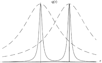
Figure 1: Resonances for $q=\frac{m}{n}$ and $q=\frac{m+1}{n}$ for two different widths, narrow resonances empedding large scale turbulent transport and broad resonances favouring strong turbulent transport.

In a quasilinear approach, the response to the perturbations will lead to large scale turbulent transport when the width of the resonance $\delta_{m}$ is comparable to the distance between the resonances $\Delta_{m,m+1}$ leading to an overlap criterion that is comparable to the well known Chirikov criterion for chaotic transport $\sigma_{m}=(\delta_{m}+\delta_{m+1})/\Delta_{m,m+1}$ with $\sigma>1$ leading to turbulent transport across the magnetic surfaces and $\sigma<1$ localising the turbulent transport to narrow radial regions in the vicinity of the resonant magnetic surfaces.

The present control schemes are two-fold. First, one can consider a large scale radial electric field that governs a Doppler shift of the mode frequency $\omega$. As such the Doppler shift $\omega-\omega_{E}$ has no effect. However a shear of the Doppler frequency $\omega_{E}$, $\omega_{E}=\bar{\omega}_{E}+\delta r\omega^{\prime}_{E}$ will induce a shearing effect of the turbulent eddies and thus control the radial extent of the mode $\delta_{m}$, so that one can locally achieve $\sigma<1$ in order to drive a transport barrier.

Second, one can modify the magnetic equilibrium so that the distance between the resonant surfaces is strongly increased in particular in a magnetic configuration with weak magnetic shear $(dq/dr\approx 0)$ so that $\Delta_{m,m+1}$ is strongly increased, $\Delta_{m,m+1}\gg\delta_{m}$, also leading to $\sigma<1$.

Both control schemes for the generation of ITBs can be interpreted using the situation sketched on figure 1. The initial situation with large scale radial transport across the magnetic surfaces (so called L-mode) is indicated by the dashed lines and is governed by significant overlap between the resonances. The ITB control scheme aims at either reducing the width of the islands or increasing the distance between the resonances yielding a situation sketeched by the plain line in figure 1 where the overlap is too small and a region with vanishing turbulent transport, the ITB, develops between the resonances.

Experimental strategies in advanced scenarios comprising Internal Transport Barriers are based on means to enforce these two control schemes. In both cases they aim at modifying macroscopically the discharge conditions to fulfill locally the $\sigma<1$ criterion. It thus appears interesting to devise a control scheme based on a less intrusive action that would allow one to modify the chaotic transport locally by the choice of an appropriate electrostatic perturbation hence leading to a local transport barrier.

2.2 The $E\times B$ model

For fusion plasmas, the magnetic field $B$ is slowly variable with respect to the inverse of the Larmor radius $\rho_{L}$ i.e: $\rho_{L}|\nabla\ln B|\ll 1$. This fact allows the separation of the motion of a charged test particle into a slow motion (parallel to the lines of the magnetic field) and a fast motion (Larmor rotation). This fast motion is named gyromotion, around some gyrocenter. In first approximation the averaging of the gyromotion over the gyroangle gives the approximate trajectory of the charged particle. This averaging is the guiding-center approximation.

In this approximation, the equations of motion of a charged test particle in the presence of a strong uniform magnetic field $\mathbf{B}=B\hat{{\sf z}}$, (where $\hat{{\sf z}}$ is the unit vector in the z direction) and of an external time-dependent electric field $\mathbf{E}=-\,\mathbf{\nabla}V_{1}$ are:

$$\frac{d}{dT}\left(\begin{array}[]{c}X\\ \\ Y\end{array}\right) = \frac{c\mathbf{E}\times\mathbf{B}}{B^{2}}=\frac{c}{B}\ \mathbf{E}(X,Y,T)\times\hat{{\sf z}}$$ (5)

$$= \frac{c}{B}\left(\begin{array}[]{c}-\partial_{Y}V_{1}(X,Y,T)\\ \\ \partial_{X}V_{1}(X,Y,T)\end{array}\right)$$ (9)

where $V_{1}$ is the electric potential. The spatial coordinates $X$ and $Y$ play the role of canonically-conjugate variables and the electric potential $V_{1}(X,Y,T)$ is the Hamiltonian for the problem. Now the problem is placed into a parallelepipedic box with dimensions $L\times\ell\times(2\pi/\omega)$, where $L$ and $\ell$ are some characteristic lengths and $\omega$ is a characteristic frequency of our problem, $X$ is locally a radial coordinate and $Y$ is a poloidal coordinate. A phenomenological model [10] is chosen for the potential:

$$V_{1}(X,Y,T)=\sum_{n,m=1}^{N}\frac{V_{0}\;\cos\chi_{n,m}}{(n^{2}+m^{2})^{3/2}}$$ (10)

where $V_{0}$ is some amplitude of the potential,

$$\chi_{n,m}\equiv\frac{2\pi}{L}nX+\frac{2\pi}{\ell}mY+\phi_{n,m}-\omega T$$

$\omega$ is constant, for simplifying the numerical simulations and $\phi_{n,m}$ are some random phases (uniformly distributed).

We introduce the dimensionless variables

$$(x,y,t)\equiv\left(2\pi X/L,\;2\pi Y/\ell,\;\omega T\right)$$ (11)

So the equations of motion (9) in these variables are:

$$\frac{d}{d{t}}\left(\begin{array}[]{c}x\\ y\end{array}\right)=\left(\begin{array}[]{c}-\partial_{y}V(x,y,t)\\ \partial_{x}V(x,y,t)\end{array}\right)$$ (12)

where $V=\varepsilon(V_{1}/V_{0})$ is a dimensionless electric potential given by

$$V(x,y,t)=\varepsilon\;\sum_{n,m=1}^{N}\frac{\cos\left(nx+my+\phi_{n,m}-t\right)}{(n^{2}+m^{2})^{3/2}}$$ (13)

Here

$$\varepsilon=4\pi^{2}(cV_{0}/B)/(L\ell\omega)$$ (14)

is the small dimensionless parameter of our problem. We perturb the model potential (13) in order to build a transport barrier. The system modeled by Eqs.(12) is a $1\frac{1}{2}$ degrees of freedom system with a chaotic dynamics [10, 6]. The poloidal section of our modeled tokamak is a Poincaré section for this problem and the stroboscopic period will be chosen to be $2\pi$, in term of the dimensionless variable $t$.

The particular choice (10) or (13) is not crucial and can be generalized. Generally, $\omega$ can be chosen depending on $n,m$. This would make the numerical computations more involved. In the following section, $V$ is chosen completely arbitrary.

3 Localized control theory of hamiltonian systems

3.1 The control term

In this section we show how to construct a transport barrier for any electric potential $V$. The electric potential $V(x,y,t)$ yields a non-autonomous Hamiltonian. We expand the two-dimensional phase space by including the canonically-conjugate variables ($E$,$\tau$),

$$H=H(E,x,y,\tau)=E+V(x,y,\tau)$$ (15)

The Hamiltonian of our system thus becomes autonomous. Here $\tau$ is a new variable whose dynamics is trivial: $\dot{\tau}=1\ {\mathrm{i.e.}}\ \tau=\tau_{0}+t$ and $E$ is the variable canonically conjugate to $\tau$. The Poisson bracket in the expanded phase space for any $W=W(E,x,y,\tau)$ is given by the expression:

$$\{W\}\equiv(\partial_{x}W)\partial_{y}-(\partial_{y}W)\partial_{x}+(\partial_{E}W)\partial_{\tau}-(\partial_{\tau}W)\partial_{E}.$$ (16)

Hence $\{W\}$ is a linear (differential) operator acting on functions of $(E,x,y,\tau)$. We call $H_{0}=E$ the unperturbed Hamiltonian and $V(x,y,\tau)$ its perturbation. We now implement a perturbation theory for $H_{0}$. The bracket (16) for the Hamiltonian $H$ is

$$\{H\}=(\partial_{x}V)\partial_{y}-(\partial_{y}V)\partial_{x}+\partial_{\tau}-(\partial_{\tau}V)\partial_{E}$$ (17)

So the equations of motion in the expanded phase space are:

$$\dot{y} = \{H\}y=\partial_{x}V(x,y,\tau)$$ (18)

$$\dot{x} = \{H\}x=-\,\partial_{y}V(x,y,\tau)$$ (19)

$$\dot{E} = \{H\}E=-\,\partial_{\tau}V(x,y,\tau)$$ (20)

$$\dot{\tau} = \{H\}\tau=1$$ (21)

We want to construct a small modification $F$ of the potential $V$ such that

$$\widetilde{H}\equiv E+V(x,y,\tau)+F(x,y,\tau)\equiv E+\widetilde{V}(x,y,\tau)$$ (22)

has a barrier at some chosen position $x=x_{0}$. So the control term

$$F=\widetilde{V}(x,y,\tau)-V(x,y,\tau)$$ (23)

must be much smaller than the perturbation (e.g., quadratic in $V$). One of the possibilities is:

$$\widetilde{V}\equiv V(x+\partial_{y}f(y,\tau),y,\tau)$$ (24)

where

$$f(y,\tau)\equiv\int_{0}^{\tau}V(x_{0},y,t)dt$$

Indeed we have the following theorem:

Theorem 1

The Hamiltonian $\widetilde{H}$ has a trajectory $x=x_{0}+\partial_{y}f(y,\tau)$ acting as a barrier in phase space.

Proof
Let the Hamiltonian $\widehat{H}\equiv\exp(\{f\})\tilde{H}$ be canonically related to $\widetilde{H}$. (Indeed the exponential of any Poisson bracket is a canonical transformation.) We show that $\widehat{H}$ has a simple barrier at $x=x_{0}$. We start with the computation of the bracket (16) for the function $f$. Since $f=f(y,\tau)$, the expression for this bracket contains only two terms,

$$\{f\}\ \equiv\ -f^{\prime}\partial_{x}\ -\ \dot{f}\partial_{E}$$ (25)

where

$$f^{\prime}\equiv\partial_{y}f\ {\mathrm{and}}\ \dot{f}\equiv\partial_{\tau}f$$ (26)

which commute:

$$[f^{\prime}\partial_{x},\dot{f}\partial_{E}]=0$$ (27)

Now let us compute the coordinate transformation generated by $\exp(\{f\})$:

$$\exp(\{f\})\;\equiv\;\exp(-f^{\prime}\partial_{x})\;\exp(-\dot{f}\partial_{E}),$$ (28)

where we used (27) to separate the two exponentials.

Using the fact that $\exp(b\partial_{x})$ is the translation operator of the variable $x$ by the quantity $b$: $[\exp(b\partial_{x})W](x)=W(x+b)$, we obtain

$$\widehat{H} = e^{\{f\}}{\tilde{H}}\;\equiv\;e^{\{f\}}E\;+\;e^{\{f\}}\tilde{V}(x,y,\tau)$$ (29)

$$= \left(E\;-\;\dot{f}\right)\;+\;\widetilde{V}\left(x-f^{\prime},y,\tau\right)$$

$$= E\;-\;V(x_{0},y,\tau)\;+\;V(x+f^{\prime}-f^{\prime},y,\tau)$$

$$= E-V(x_{0},y,\tau)+V(x,y,\tau)$$

This Hamiltonian has a simple trajectory $x=x_{0},E=E_{0}$, i.e. any initial data $x=x_{0},\ y=y_{0},E=E_{0},\tau=\tau_{0}$ evolves under the flow of $\widehat{H}$ into $x=x_{0},y=y_{t},E=E_{0},\tau=\tau_{0}+t$ for some evolution $y_{t}$ that may be complicated, but not useful for our problem. Hamilton’s equations for $x$ and $E$ are now

$$\dot{x} = \{\widehat{H}\}x=\partial_{y}\left[V(x_{0},y,\tau)-V(x,y,\tau)\right]$$ (30)

$$\dot{E} = \{\widehat{H}\}E=\partial_{\tau}\left[V(x_{0},y,\tau)-V(x,y,\tau)\right]$$ (31)

so that for $x=x_{0}$, we find $\dot{x}=0=\dot{E}$. Then the union of all points $(x,y,E,\tau)$ at $x=x_{0}\ \ E=E_{0}$:

$$\mathfrak{B}_{0}=\bigcup_{y,\tau,E_{0}}\left(\begin{array}[]{c}x_{0}\\ y\\ E_{0}\\ \tau\end{array}\right)$$ (32)

is a $3$-dimensional surface ${\mathbb{T}}^{2}\times{\mathbb{R}}$, (${\mathbb{T}}\equiv{\mathbb{R}}/2\pi{\mathbb{Z}}$) preserved by the flow of $\widehat{H}$ in the $4$-dimensional phase space. If an initial condition starts on ${\mathfrak{B}}_{0}$, its evolution under the flow $\exp(t\{\hat{H}\})$ will remain on ${\mathfrak{B}}_{0}$.

So we can say that $\mathfrak{B}_{0}$ act as a barrier for the Hamiltonian $\widehat{H}$: the initial conditions starting inside $\mathfrak{B}_{0}$ can’t evolve outside $\mathfrak{B}_{0}$ and vice-versa.

To obtain the expression for a barrier $\mathfrak{B}$ for $\widetilde{H}$ we deform the barrier for $\widehat{H}$ via the transformation $\exp(\{f\})$. As

$$\widetilde{H}=e^{-\{f\}}\widehat{H}$$ (33)

and $\exp(\{f\})$ is a canonical transformation, we have

$$\{\widetilde{H}\}=\{e^{-\{f\}}\widehat{H}\}=e^{-\{f\}}\{\widehat{H}\}e^{\{f\}}$$ (34)

Now let us calculate the flow of $\widetilde{H}$:

$$e^{t\{\widetilde{H}\}}=e^{t\left(e^{-\{f\}}\{\widehat{H}\}{e^{\{f\}}}\right)}=e^{-\{f\}}e^{t\{\widehat{H}\}}{e^{\{f\}}}$$ (35)

Indeed:

$$e^{t\left(e^{-\{f\}}\{\widehat{H}\}{e^{\{f\}}}\right)}=\sum_{n=0}^{\infty}\frac{t^{n}(e^{-\{f\}}\{\widehat{H}\}e^{\{f\}})^{n}}{n!}$$ (36)

For instance when $n=2$:

$$t^{2}(e^{-\{f\}}\{\widehat{H}\}e^{\{f\}})^{2} = t^{2}e^{-\{f\}}\{\widehat{H}\}e^{\{f\}}e^{-\{f\}}\{\widehat{H}\}e^{\{f\}}$$ (37)

$$= t^{2}e^{-\{f\}}{\{\widehat{H}\}}^{2}e^{\{f\}}$$

and so

$$e^{t\{\widetilde{H}\}}=\sum_{n=0}^{\infty}\frac{t^{n}e^{-\{f\}}\{\widehat{H}\}^{n}e^{\{f\}}}{n!}=e^{-\{f\}}e^{t\{\widehat{H}\}}{e^{\{f\}}}$$ (38)

As we have seen before:

$$e^{\{f\}}\left(\begin{array}[]{c}x\\ y\\ E\\ \tau\end{array}\right)=\left(\begin{array}[]{c}x-f^{\prime}\\ y\\ E-\dot{f}\\ \tau\end{array}\right)$$

and

$$e^{t\{\widehat{H}\}}\left(\begin{array}[]{c}x_{0}\\ y\\ E_{0}\\ \tau\end{array}\right)=\left(\begin{array}[]{c}x_{0}\\ y_{t}\\ E_{0}\\ \tau+t\end{array}\right)$$ (39)

Multiplying (35) on the right by $e^{-\{f\}}$ we obtain:

$$e^{t\{\widetilde{H}\}}e^{-\{f\}}\;=\;e^{-\{f\}}e^{t\{\widehat{H}\}}$$

$$e^{t\{\widetilde{H}\}}e^{-\{f\}}\left(\begin{array}[]{c}x_{0}\\ y\\ E_{0}\\ \tau\end{array}\right)=e^{t\{\widetilde{H}\}}\left(\begin{array}[]{c}x_{0}+f^{\prime}(y,\tau)\\ y\\ E_{0}+\dot{f}(y,\tau)\\ \tau\end{array}\right)$$ (40)

and

$$e^{-\{f\}}e^{t\{\widehat{H}\}}\left(\begin{array}[]{c}x_{0}\\ y\\ E_{0}\\ \tau\end{array}\right) = e^{-\{f\}}\left(\begin{array}[]{c}x_{0}\\ y_{t}\\ E_{0}\\ \tau+t\end{array}\right)$$ (49)

$$= \left(\begin{array}[]{c}x_{0}+f^{\prime}(y_{t},\tau+t)\\ y_{t}\\ E_{0}+\dot{f}(y_{t},\tau+t)\\ \tau+t\end{array}\right)$$ (54)

So the flow $\exp(t\{\widetilde{H}\})$ preserves the set

$$\mathfrak{B}=\bigcup_{y,\tau,E_{0}}\left(\begin{array}[]{c}x_{0}+f^{\prime}(y,\tau)\\ y\\ E_{0}+\dot{f}(y,\tau)\\ \tau\end{array}\right)$$ (55)

$\mathfrak{B}$ is a $3$ dimensional invariant surface, topologically equivalent to $\mathbb{T}^{2}\times\mathbb{R}$ into the $4$ dimensional phase space. $\mathfrak{B}$ separates the phase space into 2 parts, and is a barrier between its interior and its exterior. $\mathfrak{B}$ is given by the deformation $\exp(\{f\})$ of the simple barrier $\mathfrak{B}_{0}$.

The section of this barrier on the sub space $(x,y,t)$ is topologically equivalent to a torus $\mathbb{T}^{2}$.

This method of control has been successfully applied to a real machine: a traveling wave tube to reduce its chaos [11].

3.2 Properties of the control term

In this Section, we estimate the size and the regularity of the control term (23).

Theorem 2

For the phenomenological potential (13) the control term (23) verifies:

$$\|F\|_{\frac{1}{N},\frac{1}{N}}\leq\varepsilon^{2}N^{2}\frac{e^{3}}{4\pi}$$ (56)

if $\varepsilon$ is small enough, i.e. if $|\varepsilon|\leq\frac{\sqrt{\pi}}{2Ne^{3/2}}$ where $N$ is the number of modes in the sum (13).

Proof The proof of this estimation is given in [12] and is based on rewriting

$$F=V(x+f^{\prime})-V(x) = \int_{0}^{1}ds\ \partial_{x}V(x+sf^{\prime},y,\tau)f^{\prime}(y,\tau)$$ (57)

$$= {\mathcal{O}}(V^{2})$$

and then use Cauchy’s Theorem.

4 Numerical investigations for the control term

In this Section, we present the results of our numerical investigations for the control term $F$. The theoretical estimate presented in the previous section shows that its size is quadratic in the perturbation. Figure 2 shows the contour plot of $V(x,y,t)$ and $\widetilde{V}(x,y,t)$ ($\widetilde{V}=V+F$) at some fixed time $t$, for example $t=\frac{\pi}{4}$. One can see that the contours of both potentials are very similar. But the dynamics of the systems with $V$ and $\tilde{V}$ are very different.

For all numerical simulations we choose the number of modes $N=25$ in (13). In all plots the abscissa is $x$ and the ordinate is $y$.

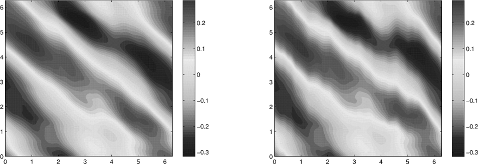
Figure 2: Uncontrolled and controlled potential for $\varepsilon=0.6$, $t=\frac{\pi}{4}$, $x_{0}=2$.

4.1 Phase portrait for the exact control term

To explore the effectiveness of the barrier, we plot (in Fig. 3) the phase portraits for the original system (without control term) and for the system with the exact control term $F$. We choose the same initial conditions. The time of integration is $T=2000$, the number of trajectories: $N_{traj}=200$ (number of initial conditions, all taken in the strip $-1-\pi\leq x\leq-\pi$; $0\leq y\leq 2\pi$) and the parameter $\varepsilon=0.9$. We choose the barrier at position $x_{0}=2$. And to get a Poincaré section, we plot the poloidal section when $t\in 2\pi{\mathbb{Z}}$. Then we compare the number of trajectories passing through the barrier during this time of integration for each system. We eliminate the points after the crossing. For the uncontrolled system $68\%$ of the initial conditions cross the barrier at $x_{0}=2$ and for the controlled system only $1\%$ of the trajectories escape from the zone of confinement. The theory announces the existence of an exact barrier for the controlled system: these escaped trajectories ($1\%$) are due to numerical errors in the integration.

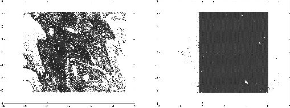
Figure 3: Phase portraits without control term and with the exact control term, for $\varepsilon=0.9$, $x_{0}=2$, $N_{traj}=200$.

One can observe that the barrier for the controlled system is a straight line. In fact this barrier moves, its expression depends on time:

$$x=x_{0}+f^{\prime}(y,t)$$ (58)

But when $t\in 2\pi{\mathbb{Z}}$ its oscillation around $x=x_{0}$ vanishes: $f^{\prime}(y,2k\pi)=\int_{0}^{2k\pi}\partial_{y}V(x_{0},y,t)dt=0$. This is what we see on this phase portrait. In fact we create $2$ barriers at position $x=x_{0}$, and $x=x_{0}-2\pi$ (and also at $x_{0}+2n\pi$) because of the periodicity of the problem. We note that the mixing increases inside the two barriers. The same phenomenon was also observed in the control of fluids [13], where the same method was applied.

4.2 Robustness of the barrier

In a real Tokamak, it is impossible to know an analytical expression for electric potential $V$. So we can’t implement the exact expression for $F$. Hence we need to test the robustness of the barrier by truncating the Fourier decomposition (for instance in time) of the controlled potential.

Fourier decomposition

Theorem 3

The potential (24) can be decomposed as $\widetilde{V}=\sum_{k\in{\mathbb{Z}}}\widetilde{V}_{k}$, where

$$\widetilde{V}_{k}=\varepsilon\sum_{n,m=1}^{N}\frac{{\mathcal{J}}_{k}(n\rho)}{(n^{2}+m^{2})^{3/2}}\cos\left(\eta+k\Theta+(k-1)t\right)\\$$ (59)

with

$$\eta_{n,m}(y) = nx+my+\phi_{n,m}+n\varepsilon F_{c}$$ (60)

$$F_{c}(y) = \sum_{n,m=1}^{N}\frac{m\;\cos(K_{n,m,y})}{(n^{2}+m^{2})^{3/2}}$$ (61)

$$F_{s}(y) = \sum_{n,m=1}^{N}\frac{m\;\sin(K_{n,m,y})}{(n^{2}+m^{2})^{3/2}}$$ (62)

$$K_{m,n,y} = nx_{0}+my+\phi_{n,m}$$ (63)

and ${\mathcal{J}}_{k}$ is the Bessel’s function

$${\mathcal{J}}_{k}(n\rho)=\frac{1}{\pi}\int_{0}^{\pi}\cos\left(ku-n\rho\sin u\right)du$$ (64)

Proof We rewrite explicitly the expression (24) for our phenomenological controlled potential $\widetilde{V}(x,y,t)$:

$$\widetilde{V}(x,y,t)=\!\varepsilon\!\!\!\sum_{n,m=1}^{N}\!\!\frac{\cos\Bigl{(}n(x+f^{\prime}(y,t))+my+\phi_{n,m}-t\Bigr{)}}{(n^{2}+m^{2})^{3/2}}$$ (65)

with

$$f^{\prime}(y,t)=\varepsilon\sum_{n,m=1}^{N}\frac{m\ \Bigl{(}\cos K_{n,m,y}-\cos(K_{n,m,y}-t)\Bigr{)}}{(n^{2}+m^{2})^{3/2}}$$ (66)

With the definition (61) and (62) we have:

$$f^{\prime}(y,t)=\varepsilon(F_{c}(y)\ (1-\cos t)-F_{s}(y)\ \sin t)$$ (67)

Let us introduce

$$\rho=\varepsilon(F_{c}^{2}+F_{s}^{2})^{1/2}$$ (68)

and $\Theta$ by

$$\rho\sin\Theta\equiv-\varepsilon F_{c}(y)\hskip 42.67912pt\rho\cos\Theta\equiv-\varepsilon F_{s}(y)$$ (69)

so that

$$\widetilde{V}=\varepsilon\sum_{n,m=1}^{N}\frac{\cos\left(\eta-t+n\rho\sin(\Theta+t)\right)}{(n^{2}+m^{2})^{3/2}}$$ (70)

Using Bessel’s functions properties [14]

$$\cos(\rho\sin\Theta)=\sum_{k\in{\mathbb{Z}}}{\mathcal{J}}_{k}(\rho)\cos k\Theta$$ (71)

$$\sin(\rho\sin\Theta)=\sum_{k\in{\mathbb{Z}}}{\mathcal{J}}_{k}(\rho)\sin k\Theta$$ (72)

we get

$$\cos\left(\eta-t+n\rho\sin(\Theta+t)\right)=\sum_{k\in{\mathbb{Z}}}{\mathcal{J}_{k}(n\rho)\cos\left(\xi\right)}$$ (73)

where $\xi=\eta+k\Theta+(k-1)t$, and we finally obtain (59). The theorem is proved. $\blacksquare$

During numerical simulations we truncate the controlled potential by keeping only its first $3$ temporal Fourier’s harmonics:

$$\widetilde{V}_{tr}\!\!=\!\varepsilon\!\!\!\!\sum_{n,m=1}^{N}\!\!\!\frac{A_{0}+A_{1}\cos t+B_{1}\sin t+A_{2}\cos 2t+B_{2}\sin 2t}{(n^{2}+m^{2})^{3/2}}$$ (74)

$$A_{0}={\mathcal{J}}_{0}(n\rho)\cos(\eta+\Theta)$$

$$A_{1}={\mathcal{J}}_{0}(n\rho)\cos\eta+{\mathcal{J}}_{2}(n\rho)\cos(\eta+2\Theta)$$

$$B_{1}={\mathcal{J}}_{0}(n\rho)\sin\eta-{\mathcal{J}}_{2}(n\rho)\sin(\eta+2\Theta)$$

$$A_{2}={\mathcal{J}}_{3}(n\rho)\cos(\eta+3\Theta)-{\mathcal{J}}_{1}(n\rho)\cos(\eta-\Theta)$$

$$B_{2}=-{\mathcal{J}}_{3}(n\rho)\sin(\eta+3\Theta)-{\mathcal{J}}_{1}(n\rho)\sin(\eta-\Theta)$$

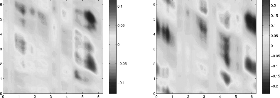
Figure 4: Exact Control Term and Truncated Control Term with $\varepsilon=0.6,t=\frac{\pi}{4}$.

Figure 4 compares the two contour plots for the exact control term and the truncated control term (74). Figure5 compares the two phase portraits for the system without control term and for the system with the above truncated control term (74). The computation of $\widetilde{V}_{tr}$ on some grid has been performed in Matlab and the numerical integration of the trajectories was done in C.

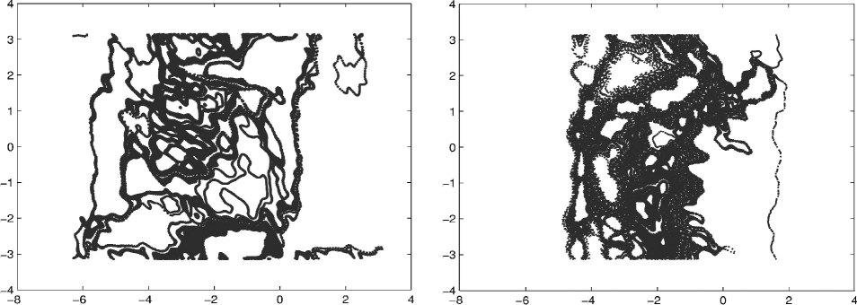
Figure 5: $\varepsilon=0.3$, $T=2000$, $N_{traj}=50$.

One can see a barrier for the system with the truncated control term. As for the system with the exact control term we create two barriers at positions $x=x_{0}$ and $x=x_{0}-2\pi$ and the phenomenon of increasing the mixing inside the barriers persist.

4.3 Energetical cost

As we have seen before, the introduction of the control term into the system can reduce and even stop the diffusion of the particles through the barrier. Now we estimate the energy cost of the control term $F$ and the truncated control term $F_{tr}\equiv\widetilde{V}_{tr}-V$.

Definition 1

The average of any function $W=W(x,y,\tau)$ is defined by the formula:

$$<|W|>=\int_{0}^{2\pi}\!\!dx\!\!\int_{0}^{2\pi}\!\!dy\!\!\int_{0}^{2\pi}\!\!dt\ |W(x,y,t)|$$ (75)

Now we calculate the ratio between the absolute value of the truncated control (electric potential) or the exact control and the uncontrolled electric potential:

$$\zeta_{ex}=<|F|^{2}>/<|V|^{2}>$$

and

$$\zeta_{tr}=<|F_{tr}|^{2}>/<|V|^{2}>$$

We also compute the ratio between the energy of the control electric field and the energy of the uncontrolled system in their exact and truncated version

$$\eta_{ex}=<|\nabla{F}|^{2}>/<|\nabla{V}|^{2}>$$

and

$$\eta_{tr}=<|\nabla{F}_{tr}|^{2}>/<|\nabla{V}|^{2}>$$

for different values of $\varepsilon$. Results are shown in Table 1.

Table 1: Squared ratios of the amplitudes of the control term and the uncontrolled electric potential $\zeta_{ex},\zeta_{tr}$; ratios of electric energy of the control term and the uncontrolled electic potential $\eta_{ex},\eta_{tr}$; for the system with exact and truncated control term.

$\varepsilon$	$\zeta_{ex}$	$\zeta_{tr}$	$\eta_{ex}$	$\eta_{tr}$
$0.3$	$0.1105$	$0.1193$	$0.6297$	$0.1431$
$0.4$	$0.1466$	$0.1583$	$0.7145$	$0.2393$
$0.5$	$0.1822$	$0.1967$	$0.8161$	$0.3550$
$0.6$	$0.2345$	$0.2137$	$0.9336$	$0.4883$
$0.7$	$0.2518$	$0.2716$	$1.0657$	$0.6375$
$0.8$	$0.2858$	$0.3038$	$1.2119$	$0.8014$
$0.9$	$0.3191$	$0.3439$	$1.3722$	$0.9796$
$1.5$	$0.5052$	$0.5427$	$2.6247$	$2.3037$

One can see that the truncated control term needs a smaller energy than the exact control term. In Table 2, we present the number of particles passing through the barrier in function of $\varepsilon$, after the same integration time.

Table 2: Number of escaping particles without control term ${\mathcal{N}}_{without}$, and for the system with the exact control term ${\mathcal{N}}_{exact}$ and the truncated control term ${\mathcal{N}}_{tr}$.

$\varepsilon$	${\mathcal{N}}_{without}$	${\mathcal{N}}_{exact}$	${\mathcal{N}}_{tr}$
$0.4$	$22\%$	$0\%$	$6\%$
$0.5$	$26\%$	$0\%$	$18\%$
$0.9$	$68\%$	$1\%$	$44\%$
$1.5$	$72\%$	$1\%$	$54\%$

Let $\Delta{\mathcal{N}}={\mathcal{N}}_{without}-{\mathcal{N}}_{tr}$ be the difference between the number of particles passing through the barrier for the system without control and with the truncated control and $\Delta\eta=\eta_{ex}-\eta_{tr}$ the difference between the relative electric energy for the system with the exact control term and the system with the truncated control term. In Table 3 we present $\Delta{\mathcal{N}}$ and $\Delta\eta$ for differents values of $\varepsilon$.

Table 3: Difference $\Delta\mathcal{N}$ of the number of particles passing trough the barrier and difference of relative electric energy $\Delta\eta$ for the controlled and uncontrolled system.

$\varepsilon$	$\Delta{\mathcal{N}}$	$\Delta\eta$
$0.3$	$8\%$	$0.49$
$0.4$	$16\%$	$0.47$
$0.5$	$8\%$	$0.46$
$0.9$	$24\%$	$0.39$
$1.5$	$18\%$	$0.32$

For $\varepsilon$ below $0.2$ the non controlled system is rather regular, there is no particles stream through the barrier, so we have no need to introduce the control electric field. For $\varepsilon$ between $0.3$ and $0.9$ the truncated control field is quite efficient, it allows to drop the chaotic transport through the barrier by a factor $8\%$ to $24\%$ with respect to the uncontrolled system and it requires less energy than the exact control field. For $\varepsilon$ greater than $1$ the truncated control field is less efficient than the exact one, because the dynamics of the system is very chaotic. For example when $\varepsilon=1.5$, there are $72\%$ of the particles crossing the barrier for the uncontrolled system and $54\%$ for the system with the truncated control field. At the same time the energetical cost of the truncated control field is above $70\%$ of the exact one, which allows to stop the transport through the barrier. So for $\varepsilon\geq 1$ we need to use the exact control field rather than the truncated one.

5 Discussion and Conclusion

In this article, we studied a possible improvement of the confinement properties of a magnetized fusion plasma. A transport barrier conception method is proposed as an alternative to presently achieved barriers such as the H-mode and the ITB scenarios. One can remark, that our method differs from an ITB construction. Indeed, in order to build-up a transport barrier, we do not require a hard modification of the system, such as a change in the q-profile. Rather, we propose a weak change of the system properties that allow a barrier to develop. However, our control scheme requires some knowledge and information relative to the turbulence at work, these having weak or no impact on the ITB scenarios.

5.1 Main results

First of all we have proved that the local control theory gives the possibility to construct a transport barrier at any chosen position $x=x_{0}$ for any electric potential $V(x,y,t)$. Indeed, the proof given in section 3 does not depend on the model for the electric potential $V$. In Subsection 3.1, we give a rigorous estimate for the norm of the control term $F$, for some phenomenological model of the electric potential. The introduction of the exact control term into the system inhibits the particle transport through the barrier for any $\varepsilon$ while the implementation of a truncated control term reduces the particle transport significantly for $\varepsilon\in(0.3,1.0)$.

5.2 Discussion, open questions

5.2.1 Comparison with the global control method

Let us now compare our approach with the global control method [6] which aims at globally reducing the transport in every point of the phase space. Our approach aims at implementing a transport barrier. However, one also observes a global modification of the dynamics since the mixing properties seem to increase away from the barriers.

Furthermore, in many cases, only the first few terms of the expansion of the global control term [6] can be computed explicitly. Here we have an explicit exact expression for the local control term.

5.2.2 Effectiveness and properties of the control procedure

In subsection 2.2, we have introduced the dimensionless variables (11) and defined a dimensionless control parameter $\varepsilon\equiv 4\pi^{2}(cV_{0}/B)/(L\ell\omega)$. In the simplifying case where $l=L=2\pi/k$ is the characteristic length of our problem, we have $\varepsilon=ck^{2}V_{0}/(\omega B)$. Let us consider a symmetric vortex, hence with characteristic scale $1/k$. Let us now consider the motion of a particle governed by such a vortex. The order of magnitude of the drift velocity is therefore $v_{E}=kcV_{0}/B$ and the associated characteristic time $\tau_{ETT}$, $\tau_{ETT}\equiv 1/(kv_{E})$, is the eddy turn over time. Let $\omega$ be the characteristic evolution frquency of the turbulent eddies, here of the electric field, then the Kubo number $K$ is $K=1/\omega\tau_{ETT}$. This parameter is the dimensionless control parameter of this class of problems, and we remark that in our case $K=\varepsilon$. It is also important to remark that the parameter $K$ also characterises the diffusion properties of our system. Indeed, let $\delta$ be a step size of our particle in a random walk process and let $\tau$ be the associated characteristic time, the diffusion coefficient is then $D=\delta^{2}/\tau$. Since one can relate the characteristic step and time by the velocity, $\delta=v_{E}\tau$, on also finds:

$$D=\frac{(v_{E}\tau)^{2}}{\tau}=\frac{k^{2}c^{2}V_{0}^{2}}{B^{2}}\tau=\frac{1}{k^{2}\tau_{ETT}^{2}}\tau=\frac{K^{2}}{k^{2}}\omega^{2}\tau$$ (76)

We also introduce the reference diffusion coefficient $\bar{D}=k^{-2}\omega$, so that:

$$D/\bar{D}\equiv K^{2}\omega\tau$$ (77)

They are two asymptotic regimes for our system. The first one, is the regime of weak turbulence, characterised by $\omega\tau_{ETT}\gg 1$ and therefore $K\ll 1$. In this regime, the electric potential evolution is fast, the particle trajectories only follow the eddy geometry on distances much smaller than the eddy size. The steps $\delta$ are small and the characteristic time $\tau$ of the random walk such that $\omega\tau\approx 1$. The particle diffusion (77) is then such that:

$$D/\bar{D}\approx K^{2}~{}~{}~{}~{}for~{}~{}~{}~{}~{}~{}\omega\tau_{ETT}\gg 1$$ (78)

The second asymptotic regime is the regime of strong turbulence, with $\omega\tau_{ETT}\ll 1$ and $K\gg 1$. Particles then explore the eddies before decorrelation and the characteristic time of the random step is typically $\tau\approx\tau_{ETT}$ and:

$$D/\bar{D}\approx K~{}~{}~{}~{}for~{}~{}~{}~{}~{}~{}\omega\tau_{ETT}\ll 1$$ (79)

The first regime corresponds to the weak turbulence limit with weak Kubo number and particle diffusion and the second to strong turbulence and large Kubo number and particle diffusion. The control method developed in this article does not depend on $K\equiv\varepsilon$. There is always a possibility to construct an exact transport barrier. However for the numerical simulations, we have remarked, that for small $\varepsilon$ one can observe a stable barrier without escaping particles, and for $\varepsilon$ close or more than $1$ there is some leaking of particles across the barrier. The barrier is more difficult to enforce. Also when considering the truncated control term, one finds that the control term is ineffective in the strong turbulence limit.

Let us now consider the implementation of our method to turbulent plasmas where the turbulent electric field is consistent with the particle transport. The theoretical proof of an hamiltonian control concept is developped provided the system properties at work are completely known. For example the analytic expression for the electric potential. This is impossible in a real system, since the measurements take place on a finite spatio-temporal grid. This has motivated our investigation of the truncated control term by reducing the actually used information on the system. As pointed out previously, one finds that this approach is ineffective for strong turbulence. Another issue is the evolution of the turbulent electric field following the appearance of a transport barrier. This issue would deserve a specific analysis and very likely updating the control term on a trasnport characteristic time scale. An alternative to such a process would be to use a retroactive Hamiltonian approach (a classical field theory) [15] and to develop the control theory in that framework.

Acknowledgements

We acknowledge very useful and encouraging discussions with A. Brizard, M. Vlad and M. Pettini. This work supported by the European Communities under the contract of Association between EURATOM and CEA was carried out within the framework of the European Fusion Development Agreement. The views and opinions expressed herein do not necessarily reflect those of the European Commission.

References

- [1] F. Wagner and U. Stroth, Plasma Phys. Contr. Fusion, 35, 1321 (1993).
- [2] M. Shimada et al., Nucl. Fus.,47 S1 (2007).
- [3] F. Wagner et al., Phys. Rev. Lett.,49,1408 (1982)
- [4] C. Gormezano et al., Nucl. Fus.,47 S285 (2007).
- [5] E.J. Doyle et al., Nucl. Fus.,47 S18 (2007).
- [6] G. Ciraolo, F. Briolle, C. Chandre, E. Floriani, R. Lima, M. Vittot, M. Pettini, Ch. Figarella, Ph. Ghendrih: “Control of Hamiltonian chaos as a possible tool to control anomalous transport in fusion plasmas”, Phys. Rev. E, 69, 056213 (2004).
- [7] J. Wesson, Tokamaks, Oxford University Press (2004).
- [8] G. Fiksel et al., Phys. Plasmas., 2, 4586 (1995).
- [9] X. Garbet et al., Nucl. Fus., 47, 1206 (2007).
- [10] M. Pettini, A. Vulpiani, J. H. Misguich, M. De Leener, J. Orban, R. Balescu: “Chaotic diffusion across a magnetic field in a model of electrostatic turbulent plasma”, Phys. Rev. A 38, (1988) p 344-363.
- [11] C. Chandre, G. Ciarolo, F. Doveil, R. Lima, A. Macor, M. Vittot: “Channelling chaos by building barriers”, Phys. Rev. Lett. 94, 074101 (2005).
- [12] N. Tronko, M. Vittot: “Localized control theory for hamiltonian systems and its application to the chaotic transport of test particules in plasmas”. To appear in the proceedings of the “Joint Varenna - Lausanne International Workshop: Theory of Fusion Plasmas”, Varenna (August 2008)
- [13] T. Benzekri, C. Chandre, X. Leoncini, R. Lima, M. Vittot: “Chaotic advection and targeted mixing”, Phys. Rev. Lett. 96, 124503 (2006).
- [14] M. Abramowitz, I. A. Stegun, eds. Handbook of Mathematical Functions, (Dover, New York, 1965), p 361.
- [15] I. Bialynicki-Birula, J. C. Hubbard, L. A. Turski: “Gauge-independent canonical formulation of relativistic plasma theory”, Physica A 128 (1984) p 509-519.