QUASISTATIC RHEOLOGY AND THE ORIGINS OF STRAIN.

Abstract

Features of rheological laws applied to solid-like granular materials are recalled and confronted to microscopic approaches via discrete numerical simulations. We give examples of model systems with very similar equilibrium stress transport properties – the much-studied force chains and force distribution – but qualitatively different strain responses to stress increments. Results on the stability of elastoplastic contact networks lead to the definition of two different rheological regimes, according to whether a macroscopic fragility property (propensity to rearrange under arbitrary small stress increments in the thermodynamic limit) applies. Possible consequences are discussed.

RÉSUMÉ : On confronte l’approche microscopique par simulation numérique discrète des matériaux granulaires de type solide à leurs propriétés rhéologiques macroscopiques. On cite des systèmes modèles dont les réponses, en déformation, un incrément de contrainte diffèrent qualitativement, bien que la répartition des efforts l’équilibre soit très similaire. Des résultats sur la sensibilité aux perturbations des réseaux de contact élastoplastiques permettent de distinguer deux régimes rhéologiques, selon que leurs intervalles de stabilité, en termes de contraintes, se réduisent ou non zéro dans la limite thermodynamique (‘fragilité’ macroscopique). On en évoque de possibles conséquences.

MOTS-CLÉS : Déformation, loi de comportement, simulations numériques

KEYWORDS: Strain, constitutive law, numerical simulations

1 Scope

This is a brief introduction to the rheology of solid-like granular materials in the quasistatic regime, with a special emphasis on the microscopic origins of strain, and on discrete numerical simulations of model systems. Rather sophisticated macroscopic phenomenological laws have been proposed [1, 2, 3], but, in spite of many microscopic studies [4, 5], with numerical tools [7] in particular, their relation to grain-level physical phenomena is not fully understood. Consequently, we mostly address basic, qualitative aspects on model systems. Moreover, we specialize on cohesionless, nearly rigid grains, and to small or moderate strain levels (excluding continuous, unbounded plastic flow). Despite the many insufficiencies of present-day modelling attempts, interesting directions for future research, elaborating on preliminary results, can be suggested. We recall a few basic concepts (section 2), some of the macroscopic phenomenology of solid-state granular mechanics (part 3), and the necessary elements of a microscopic model (section 4). Then, properties of simple model systems studied by numerical means, in the large system limit, are discussed both in frictionless (section 5) and in frictional (section 6) systems. Section 7 suggests broader perspectives and speculations.

2 The constitutive law approach: basic ideas.

On setting out to identify a constitutive law for a solid material, one has to rely on some postulates that are worth recalling in the context of granular materials. Such a law should locally relate stresses $\underline{\underline{\sigma}}$ to strains $\underline{\underline{\epsilon}}$ , or, more appropriately for granular systems, stress rates $\underline{\underline{\dot{\sigma}}}$ and strain rates $\underline{\underline{\dot{\epsilon}}}$ should determine each other for a given internal state of the system. This state is to be conceived of as specified once the values of some state variables (a finite number $p$ of quantities, including the stress tensor itself, that exhaust the macroscopic description of the system) are known. One may write, at each time $t$:

$$\underline{\underline{\dot{\sigma}}}({\bf x},t)={\mathcal{F}}\left(\underline{\underline{\dot{\epsilon}}}({\bf x},t),\underline{\underline{\sigma}}({\bf x},t),\left\{\alpha({\bf x},t)\right\}\right)\mbox{\ \ or \ \ }\underline{\underline{\dot{\epsilon}}}({\bf x},t)={\mathcal{G}}\left(\underline{\underline{\dot{\sigma}}}({\bf x},t),\underline{\underline{\sigma}}({\bf x},t),\left\{\alpha({\bf x},t)\right\}\right)$$ (1)

${\bf x}$ standing for any ‘point’, in the sense of continuum mechanics, in the sample, i.e. a representative volume element from the microscopic point of view. $\{\alpha\}$ is the set of unspecified state variables $(\alpha_{i})_{1\leq i\leq p}$. Their evolution should be ruled by similar equations:

$$\dot{\alpha}_{i}({\bf x},t)={\mathcal{H}}\left(\underline{\underline{\dot{\epsilon}}}({\bf x},t),\underline{\underline{\sigma}}({\bf x},t),\left\{\alpha({\bf x},t)\right\}\right).$$ (2)

Once eqns. 1 and 2 are given, and supplemented with the appropriate boundary conditions, one also needs the initial values of $\underline{\underline{\sigma}}$ and $\alpha$ to be able to predict the evolution of the system for, say, a prescribed history of stress. The prediction of the initial state of the system is in general beyond the scope of the rheological laws we are dealing with, as it is the result of a process that might involve rapid flow. (One exception is the construction of a sample under gravity by successive deposition of thin layers at the free surface. If the initial state of a freshly deposited layer is known, one may apply solid-like rheology to the rest of the sample, which deforms very little under the weight of the new layer, and thus, iteratively solving the appropriate boundary value problem, calculate the initial state of a whole system as a result of its construction history. This procedure can be applied to silos [8] and granular piles [9]).

The suggestions, put forward in the recent literature [10], to look for direct relationships between stress components that result from the construction history of a sample, are attempts to model the assembling procedure, rather than the response to stress increments. The proposed relations are not constitutive laws in the sense of eqns. 1 and 2: they ignore strains, and they are not local (they depend on sample shape and boundary conditions).

One thus needs some a-priori knowledge of the initial stresses: however small the components of the stress tensor, the orientation of its principal axes and its level of anisotropy are important. Cohesionless grains do not spontaneously assemble in any ‘natural state’, once submitted to some externally imposed stresses they form packings the structure of which depends on those stresses. Functions ${\mathcal{F}}$, ${\mathcal{G}}$ and ${\mathcal{H}}$ of relations 1 and 2 must be discontinuous at $\underline{\underline{\sigma}}=0$. In rheometric experiments one needs in principle to check for sample homogeneity.

3 Macroscopic aspects

Constitutive laws like eqns. 1 and 2 are studied in soil mechanics [3, 5, 6]. In order to extract some information on such laws from experiments, it is convenient to choose configurations in which stresses and strains are expected to be homogeneous. This leads to the design of rheometers, the most often employed one in soil mechanics being the triaxial apparatus, sketched on fig. 1.

\psfrag{v}[c]{$\dot{\epsilon}_{1}$, $\sigma_{1}$}\psfrag{a}[c]{$\sigma_{3}$}\includegraphics[width=142.26378pt]{fig1.eps}

Figure 1: Sketch of a triaxial experiment.

Samples are submitted to axisymmetric states of stress, the axial stress $\sigma_{1}$, or the axial strain $\epsilon_{1}$, are controlled via the relative motion of the end platens, while the lateral pressure $p=\sigma_{2}=\sigma_{3}$ is exerted through a flexible membrane by a fluid. With some care (e.g., measuring strains directly on the sample in the central part away from the rigid platens) it is possible, with the most sophisticated devices, to record strains with an accuracy of the order of $10^{-6}$ [11, 12]. Other rheometers [13] are the ‘true triaxial’ apparatus, which may impose three different principal stresses to a cubic sample, and the ‘hollow cylinder’ apparatus, which allows for rotation of the principal axes of stress and strain. In a typical triaxial experiment, one starts from a given state with, e.g., hydrostatic stress ($\underline{\underline{\sigma}}=p\underline{\underline{{\bf 1}}}$). Then, most often, $\epsilon_{1}$ is increased at a constant (slow) rate, while lateral pressure $p$ is maintained constant. Axial stress $\sigma_{1}$ – or, equivalently, deviator $q=\sigma_{1}-p$ – and the lateral strain $\epsilon_{2}=\epsilon_{3}$ (or, equivalently, the relative volume increase, $\epsilon_{v}=-tr(\underline{\underline{\epsilon}})$) are measured. Evolutions of $q$ and $\epsilon_{v}$ as $\epsilon_{1}$ monotonically increases are schematically represented on fig. 2.

\psfrag{x}[l]{$\epsilon_{1}$}\psfrag{y1}[l]{$q=\sigma_{1}-\sigma_{3}$}\psfrag{y2}[l]{$-\epsilon_{v}$}\psfrag{p}[l]{\footnotesize`peak'}\includegraphics[width=156.49014pt]{fig2.eps}

Figure 2: Schematic variations of deviator $q$ (continuous curves) and volumetric strain $\epsilon_{v}$ (dotted lines) for a dense and a loose sand. The curve marked with arrows is observed on decreasing $q$ or $\epsilon_{1}$.

While the density and the deviator steadily increase, in a loose sample, until asymptotic constant values are reached, dense samples are initially contractant, then dilatant and the deviator curve passes through a maximum. From the beginning, the increase of $q$ with $\epsilon_{1}$ is not reversible: if the direction of deformation is reversed, the same curve is not retraced back: the decrase of the deviator is steeper, with a slope comparable to that of the tangent at the origin of coordinates on fig 2.

As $\epsilon_{1}$ increase, the curves approach a plateau, corresponding to a final attractor that is called the ‘critical state’ [3] and deemed independent of the initial conditions (density and deviator should coincide for the loose and the dense sample on fig. 2 at large $\epsilon_{1}$). However, the approach to this critical state is often hidden, in dense samples at least, by instabilities leading to strain localization in ‘shear bands’ (whose thickness is of the order of a few grain diameters). The development of these localizations was observed by X-ray tomography [14]. It is sensitive to sample shape and boundary conditions, but usually occurs in the vicinity of the observed ‘stress peak’. Localization in loose samples, if it exists, is far less conspicuous. As sample homogeneity is lost, localization precludes the interpretation of rheometric tests in terms of constitutive laws, which should therefore be restricted to the ‘pre-peak’ part of the curve.

An important feature of rheological tests on solid-like granular samples is their independence on physical time (see however, the remarks of section 7). Replacing $t$ by $\varphi(t)$ with a monotonically increasing function $\varphi$ does not change stress-strain curves. Functions ${\mathcal{F}}$, ${\mathcal{G}}$ , ${\mathcal{H}}$ should therefore be homogeneous of degree one in $\underline{\underline{\dot{\epsilon}}}$ or in $\underline{\underline{\dot{\sigma}}}$. Such tests are supposed to be quasi-static, as a sequence of equilibrium states is explored. Dynamical characteristics, such as masses, are regarded as irrelevant. Dry sands and water-saturated ones, provided static properties are the same, should exhibit the same behaviour.

Eqns. 1 and 2, with due account for material symmetries, remain extremely general. The nature of internal variables $\alpha$ is not easy to guess if only stresses and strains are measured. The packing fraction is often chosen, because of its influence on the behaviour (fig. 2).

To account for irreversibilies and failure, the most commonly invoked laws are of the elastoplastic family. Those (although usually written differently) can be cast in the form of eqns. 1 and 2. We do not review elastoplasticity here. Its application to soil mechanics is presented in ref. [3]. Connections to limit analysis (calculation of a limit load beyond which unlimited plastic flow occurs) are discussed in [15]. Ref. [16] is a pedagogical introduction with examples of calculations with simplified laws. The complex behaviour sketched on fig. 2 requires quite sophisticated elastoplastic laws, with many parameters. Those laws should be non-associated [16], and involve work hardening. Very roughly speaking, this means that the direction of plastic irreversible strains is not simply related to the failure condition on stresses, and that failure is a gradual process. A simplified law with correct qualitative properties in terms of global failure under monotonically varying loads [16] involves 4 parameters. A more elaborate and quantitative one, Nova’s law [17], requires 8 parameters. Incremental [1] or hypoplastic [18] laws are less traditional. They directly state relations like eqns. 1 and 2. ${\mathcal{F}}$ and ${\mathcal{G}}$, although positively homogeneous of degree one, should be non-linear functions of $\underline{\underline{\dot{\epsilon}}}$ and $\underline{\underline{\dot{\sigma}}}$ respectively, to account for irreversibility. This is directly postulated in such approaches, while elastoplastic laws describe such a behaviour through work hardening. Ref. [18] defines a simplified hypoplastic law with 5 parameters.

Obviously, it is highly desirable to identify parameters with a physical meaning, connected with the microscopic mechanisms of deformation under stress. This would ease and guide the choice of a constitutive law, contribute to assess its range of validity (e.g., in terms of stress magnitudes), and reveal the influence of microscopic characteristics of a given material on its macroscopic behaviour.

4 Ingredients of a microscopic model, discrete simulations.

Numerical simulation methods are described in ref. [7]. They deal with simple models of granular materials, suitable to investigate the microscopic origins of constitutive laws. Here, we mainly discuss the simple cases of discs (2D) or spheres (3D). Three different kinds of ingredients are needed: geometric, static and dynamical ones. First, grain shape and polydispersity have to be specified. Then, static parameters are those defining equilibrium contact laws. In the most simple model, a normal stiffness constant $K_{N}$ expresses a proportionality between normal force $f_{N}$ and normal deflection $h$ of a contact (which is modelled as an interpenetration depth), a tangential stiffness $K_{T}$ incrementally relates tangential contact forces $f_{T}$ to tangential relative displacements, and Coulomb’s condition $|f_{T}|\leq\mu f_{N}$ should be satisfied, with a friction coefficient $\mu$, sliding being allowed (such that the work of $f_{T}$ is negative) if it holds as an equality. One may regard stiffness constants as a mere computational trick to forbid grain interpenetration. They may also be chosen with correct order of magnitudes, comparing them to typical estimated values of $df_{N}/dh$ in contacts, under some given stress level. It can even be attempted to implement accurate contact laws, such as the Hertz-Mindlin-Deresiewicz [19] ones for smooth elastic spheres with friction.

Finally dynamical parameters are related to inertia (masses, moments of inertia) and kinetic energy dissipation (e. g. viscous damping in contacts). In slow, quasi-static evolutions, those parameters should be irrelevant, the behaviour should be determined by the geometric data, along with $\mu$, ratio $K_{T}/K_{N}$ and parameter $K_{N}/P$ (in 2D) or $K_{N}/(Pd)$ (in 3D), which measures the deflections of contacts relative to grain diameter $d$ under typical forces [24].

The most widely used simulation methods [7], molecular dynamics (MD), or contact dynamics, rely on time integration of dynamical equations of motion. They have been used to simulate biaxial (in 2D) [20] or triaxial [21] tests. Such calculations are usually made at constant axial strain rate, assuming the system remains close enough to equilibrium at any time for the evolution to be regarded as quasi-static. They cope with a few hundreds or a few thousands of grains. They successfully produce stress-strain curves whose broad features, on the scale of $\epsilon\sim 10\%$, are those of fig. 2. For instance Thornton’s simulations [21] yield a maximum deviator criterion that coincides with some experimental observations. However, stress-strain curves, for given loading histories, are still rather noisy on a smaller scale ($\epsilon\sim 1\%$), especially as the peak is approached (strain values corresponding to the peak deviator are not accurate). It seems necessary to study the form of such curves and investigate the regression of fluctuations with greater care, for two reasons: first, one might wish to obtain accurate estimations of rheological laws in the macroscopic limit; then reliable numerical data on the effect of perturbations on equilibrium states would give insight on the microscopic mechanisms of deformation. Those should be accounted for in theoretical attempts to relate rheological laws to grain-level phenomena. The next sections are therefore devoted to biaxial compressions with 2D systems of disks, in which deviator $q=\sigma_{1}-\sigma_{2}$ (keeping the notations introduced for the triaxial test) is stepwise increased and one studies the effect of small stress increments imposed on equilibrium configurations.

5 Response to stress increments: frictionless grains

Assemblies of frictionless grains are particularly appealing because of two remarkable properties, that are established and discussed in ref. [22]. The first one, the absence of hyperstaticity in the limit of large contact stiffness, means that the contact network is barely sufficient to support stresses, and that the sole condition that only closed contacts can transmit a force, along with the force (and torque) balance equations, is sufficient to calculate all contact forces. The second (the standard mechanical energy minimization property) states, for rigid grains, that the potential energy of external forces has to be minimized under the constraints of no interpenetration. It allows to discuss the stability of equilibrium states.

Together, both properties entail [22] that force-carrying structures in assemblies of rigid frictionless and cohesionless disks (in 2D) or spheres (in 3D) are isostatic: there is a one to one correspondence between external forces and contact forces, and between relative normal velocities in the contacts and grain velocities. We exploited this [23] to study the response of disordered systems of disks to stress increments, by a purely geometric procedure we called the ‘geometric quasi-static method’ (GQSM). In such systems, the stress-strain curve is a staircase and the procedure tracks the elementary steps. In stability intervals, the rigid contact structure supports the stress without motion, until one contact force becomes negative. This contact has then to open, initiating a rearrangement, hence a strain increment. Motion stops when another contact closes and a new stable equilibrium is reached. In fact, this might require several contact replacements, which are operated one by one in this algorithm. On opening one contact, the ensuing velocity field is, up to a positive factor, geometrically determined. One example is displayed on fig. 3.

Figure 3: Velocity field at the beginning of a rearrangement in a system of 1024 disks in a square box undergoing biaxial compression. The contact between the disks marked in gray (bottom right) is opening.

Those fields form complex vortex patterns extending through the whole sample. Displacement fields corresponding to small strain increments have the same aspect.

Statistics of stress and strain steps for the beginning of a biaxial compression (close to the isotropic state of stress) were studied [23, 24]. It was found that intervals of stability $\delta q$ are exponentially distributed and scale with the number of disks $N$ as $N^{-\alpha}$ with $\alpha\simeq 1.1$, while ‘axial’ (conjugate to the largest principal stress that is being incremented) strain steps are power-law distributed, the density function decrasing as $(\delta\epsilon)^{-(1+\mu)}$, with $\mu\simeq 0.5$ for large values, and scale as $N^{-\beta}$ with $\beta\simeq 2.1$.

As stability regions in stress space dwindle to nothing in the thermodynamic limit (a macroscopic ‘fragility’ property [25, 22]), equilibrium states will be rather elusive: it is impossible, in a real experiment, to control stress levels with perfect accuracy. Although each equilibrium configuration is rigid, any level of noise in a macroscopic system should generate fluctuations, because rigid configurations become unstable, and the system should keep visiting several equilibrium states.

Since the power law distribution of strain increments does not admit a mean value, the accumulation of successive $\delta\epsilon$ steps generates a Lévy process [26], and the strain step corresponding to a given deviator increment remains impredictable. Although, as $N$ increases, the typical size of steps decreases, the staircase stress-strain curve does not become smooth because of the statistical importance of large strain increments. It was also observed [23] that the statistics of strain variations corresponding to given stress intervals do not depend on $N$. Moreover, this distribution is the same for the GQSM and for a more conventional MD calculation (with nearly rigid grains, $K_{N}/P=10^{5}$). As MD results, introducing additional static and dynamical parameters, are statistically indistinguishable from GQSM ones, one may conclude that the mechanical response is determined by geometry alone. These results are summarized on fig. 4

Figure 4: Distribution of axial strain increments corresponding to fixed $\Delta q=10^{-3}p$ measured for 4 sample sizes (up to $N=4900$) with GQSM and 2 sizes (1000 and 3000) with MD. Note the independence on the numerical method (for large values) and the absence of convergence, as $N$ increases, to a deterministic response.

This very singular behaviour – a constitutive law cannot be defined – calls for additional investigation of its origins and range of validity. It is worth pointing out that the observation of the large $\delta\epsilon$ values and the Lévy-stable distribution are due to the rearrangements in which several (sometimes many) contacts have to be replaced. If we now adopt the approximation of small displacements (ASD) in which displacements away from a reference configuration are dealt with as infinitesimal, and hence normal unit vectors between neighbouring disks are kept constant, then it can be shown [22] that only one contact replacement will be enough to reach the next equilibrium state. Then, the distribution of strain steps admits a first and a second moment, and the staircase, within the ASD, should approach a smooth curve.

In fact, the ASD with frictionless grains has deep consequences: it entails [22] the uniqueness of equilibrium states. There is no need to obtain a stress-strain curve in an incremental way, as stresses and strains are in one-to-one correspondence. Uniqueness also implies the absence of irreversibility, since there is no history dependence. Assemblies of slightly polydisperse disks placed on a regular triangular network were studied within the ASD (with the unperturbed lattice as reference). The approximation is well controlled in that case because of the small polydispersity parameter. This system might be called elastic (although disks are rigid). Its behaviour was shown [27, 22] to be analogous to that of a mobile point requested to stay within a convex part ${\mathcal{D}}$, limited by a smooth surface $\Sigma$, of a three-dimensional space (the analog of the set of values permitted by impenetrability conditions in strain space). Once submitted to an external force (its 3 coordinates are the analogs of the stress components) its equilibrium position is the point of $\Sigma$ where the tangent plane is orthogonal to the force. Hence a smooth correspondence between force and displacements. Upon incrementing the force, the displacement is inversely proportional to the curvature of $\Sigma$. As a consequence of these properties [22], the macroscopic response (displacements) to some small localized force superimposed on a pre-imposed stress field (Green’s function) is, for this model, the solution to an elliptic boundary value problem (akin to elastic problems for incompressible materials). Within the ASD, finding an equilibrium state amounts to solving a convex minimization problem. This is also the case, without the ASD, for networks of cables, for which the same kind of elasticity applies.

Let us summarize the main conclusions of these studies on rigid frictionless grains.

(i) The stress-strain curve is a staircase with phases of stability, with just enough contacts to carry the forces, alternating with rearrangements, with just enough contact openings to allow some deformation. Those rearrangements are non-local events, involving the whole system. (ii) Any macroscopic stress perturbation causes some rearrangement. (iii) No deterministic constitutive law applies to disordered assemblies of rigid, frictionless disks. (iv) The mechanical response is determined by the sole geometric data. (v) Different systems might exhibit equilibrium states with extremely similar properties (in terms of force distributions) and both satisfy properties i and ii. However their mechanical behaviour might be drastically different: conclusion iii applies to disks without the ASD, whereas disks within the ASD or cable networks abide by some form of elasticity, rearrangements being reversible.

6 Response to stress increments: grains with friction

Let us now report some results on disordered systems of nearly rigid ($K_{N}/P=10^{5}$) systems of disks with a friction coefficient $\mu>0$ in the contacts [28, 24]. Just like in the frictionless case, one may either try to track elementary stability intervals and rearrangements, or resort to molecular dynamics (introducing additional parameters). However, the specific properties of frictionless systems are lost: the contacts may transmit tangential forces and the network is hyperstatic; potential energy is no longer minimized at equilibrium. To discuss the stability of a given contact network, one needs to introduce elasticity in the contacts. One can then perform static elastoplastic calculations: the system is to be regarded as a network of springs, plastic sliders and no-tension joints, the displacements and rotations of the disks can be computed for each applied stress increment, via an iterative process [29]. Such studies of elastoplastic networks [29, 30] with static methods are surprisingly rare, especially in comparison to the vast literature on numerical simulations of elastic networks and brittle fracture (see e.g. [31]) The systems studied in [28] were prepared without friction, and are thus very dense. Several simple sizes were studied ($N$ ranging from $1000$ to $5000$), and it was found that the initial contact network, corresponding to isotropic stresses at the beginning of the biaxial compression, is able to support a considerable stress deviator ($q/p=0.81\pm 0.06$ for $\mu=0.25$) in the large system limit. Therefore, such dense systems with friction are not fragile in the sense of section 5. Stress-strain curves for $\mu=0.25$, $K_{T}/K_{N}=0.5$ for the beginning of the biaxial compression are shown on fig. 5. In this regime, that we call strictly quasi-static, the curve is smooth, the successive equilibrium configurations form a continuum. The scale of strains is set by the stiffness constants in the contacts. The behaviour is inelastic and irreversible from the beginning of the biaxial compression, as the proportion of sliding or opening contacts steadily increases. Eventually, some instability occurs, the initially present contacts can no longer support the stresses. Interestingly, this appears to happen for a deviator value that does not sensitively depend on stiffness constants [24]. To proceed further (as the current state of the static algorithm does not clearly determine one direction of instability and no analog of the GQSM is available), we resorted to molecular dynamics. Successive equilibria corresponding to stepwise increasing deviator values were obtained, and a staircase-like stress-strain curve was observed, signalling the frequent occurrence of instabilities and strain jumps (fig. 5).

Figure 5: Main plot: aspect of deviator/axial strain curves for $\epsilon_{1}\leq 0.02$ (MD calculations). The dotted lines are results obtained with the static method on going backwards on the same stress path ($q$ decreases). The inset – note the blown-up $\epsilon$ scales – shows $q$ and $\epsilon_{v}$ versus $\epsilon_{1}$ in the strictly quasi-static regime

To check whether a well-defined stress-strain relation is approached as $N\to\infty$, averages and mean standard deviations of $q(\epsilon_{1})$ for $0\leq\epsilon_{1}\leq 0.02$ were computed with several samples of different sizes, and the results (fig. 6) do indicate that a smooth curve is approached. Similar results are obtained for $\epsilon_{v}$ versus $\epsilon_{1}$.

Figure 6: $q(\epsilon_{1})$ for 3 sample sizes: the larger $N$, the darker is the shaded zone extending to one standard deviation above and below the average. The inset displays the average standard deviation throughout the $\epsilon_{1}$ range, for $q$ and for the volumetric strain, versus $N^{-1/2}.$

Any strictly quasi-static interval appears as a vertical segment on fig. 6. The existence of a limit for large $N$ requires in fact the fragility property to apply in the staircase regime. However, it is expected that although any positive increment $\delta q$ will entail a rearrangement in a macroscopic system, contact structures will withstand finite negative $\delta q$’s. Fig. 5 shows that relatively large $q$ intervals could be accessed by static calculations, from intermediate equilibrium configurations in the staircase regime, upon decreasing $q$. Moreover, it is observed that many contacts stop sliding on reversing the motion. It would be interesting to investigate the response to differently oriented stress increments, and to delineate the (history-dependent) strictly quasi-static, non-fragile domain around a given equilibrium state. Taking the mobilization of friction into account – i.e., replacing Coulomb’s inequality by an equality for all sliding contacts – it can be observed that the indeterminacy of forces is greatly reduced within the staircase regime in the monotonic biaxial compression [20, 28], which suggests an analogy with isostatic frictionless systems. Grain motions, rearrangements and spatial distribution of strains were studied by Williams and Rege [32], and by Kuhn [33]. Similar patterns as those of fig. 3 were observed. Thin non-persistent (unlike shear bands) ‘microbands’ concentrating the strain were also reported [33].

There is therefore some evidence that conclusions (i), (ii), and (iv) of section 5 are still valid in systems with friction within the fragile ‘staircase’ regime, the essential differences being the role of the friction coefficient itself (the behaviour appears to be essentially determined by the geometry and $\mu$), the existence of a well-defined macroscopic stress-strain curve and that of strictly quasi-static regimes within which a given network of contacts is able to support a finite stress range, all strains being due to the finite stiffness of the grains themselves.

7 Some perspectives and speculations.

The non-local aspect of rearranging events, reflecting the strong steric hindrance in dense packings of impenetrable bodies, could be expected to preclude the definition of a local law. However, one might think that a great number of such long-distance correlated motions of very small amplitudes could, once aggregated, build up a strain field devoid of long-range correlations. Specifically, strains could be localized on some ‘microband’ pattern (as reported by Kuhn [33]) during one elementary rearrangement, but the random superposition of lots of such non-persistent structures could destroy the long-distance correlations. Similar ideas were followed by Török et al. [34]: their schematic model assumes macroscopic deformation to result from an accumulation of slides on temporary slipping surfaces. It would be interesting to test such a scenario, which requires an accurate numerical computation of directions of instabilities of granular assemblies with a given contact network. That ‘deformation consists in a number of arrested slides’ is an idea already put forth by Rowe in 1962 (ref. [35],p. 514). His classical ‘stress-dilatancy relation’ [35] could thus be founded on a microscopic analysis.

In parallel to the analysis of stress-strains relationships we have been reporting here (we focussed on eqn. 1), microscopic studies have tried to define internal state variables of granular systems and to relate them to stresses and strains (i.e. suggesting a form of eqn. 2). For instance, the density of contacts and some parametrization of the distribution of their orientation (called fabric or texture) have been studied, their evolution can be related to strains [36, 37] (eqn. 2) and their values can be correlated to the possibly supported stress orientations [38] (role of $\alpha$ in eqn. 1). A brief presentation of the possible use of packing fraction and fabric as work-hardening variables in a plasticity theory is ref. [39].

Finally, let us briefly speculate about possible consequences of the existence of strictly quasi-static and fragile regimes. Sand specimens were observed to creep: under constant stresses [40, 41] (e.g., on stopping a triaxial test and maintaining constant stresses) strains vary very slowly, over hours. (Let us quote ref. [35] again: ‘The time to equilibrium increases to many days as the peak strength is approached’).

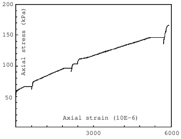
Figure 7: Axial stress vs. axial strain curve, from ref. [40]. The experiment was stopped at constant stress several times, hence the creep intervals. Note the stiff response when the constant rate compression is resumed.

A new equilibrium might be approached, which can be rather distant. When the slow controlled strain rate is resumed, the response to both positive and negative $q$ increments is quite stiff. With due account to possible aging phenomena in the contacts [42], it is tempting to suggest the following explanation: once left to wait at constant stress, the grain pack, which is highly sensitive to noise, slowly drifts in configuration space, until it reaches a state with a finite stability range (hence a stiff response of the ‘strictly quasi-static’ type). There appears thus to be interesting connections between slow dynamics and fragility.

References

- 1. Constitutive Relations for Soils, edited by G. Gudehus, F. Darve, and I. Vardoulakis (Balkema, Rotterdam, 1984).
- 2. Manuel de rhéologie des géomatériaux, edited by F. Darve (Presses des Ponts et Chaussées, Paris, 1987).
- 3. Wood D. M., Soil Behaviour and Critical State Soil Mechanics (Cambridge University Press, 1990).
- 4. Powders and Grains 2001, edited by Y. Kishino (Balkema, Lisse, 2001).
- 5. Physics of Dry Granular Media, edited by H. J. Herrmann, J. P. Hovi, and S. Luding (Balkema, Dordrecht, 1998).
- 6. Biarez, J. and Hicher, P.-Y., Elementary Mechanics of Soil Behaviour (Balkema, Rotterdam, 1994)
- 7. Cambou B. and Jean M., Micromécanique des matériaux granulaires (Hermès, Paris, 2001).
- 8. Ragneau E., Ph.D. thesis, Institut National des Sciences Appliquées, Rennes, 1993.
- 9. Boufellouh S., Ph.D. thesis, Ecole Centrale, Châtenay-Malabry, 2000.
- 10. Cates M. E., Wittmer J. P., Bouchaud J.-P., and Claudin P., Phil. Trans. Roy. Soc. London 356, 2535–2560 (1998).
- 11. Di Benedetto H., Geoffroy H., Sauzéat C., and Cazacliu B., in Pre-failure Deformation Characteristics of Geomaterials, edited by M. Jamiolkowski, R. Lancellotta, and D. Lo Presti (Balkema, Rotterdam, 1999), pp. 89–96.
- 12. Hicher P.-Y., ASCE J. Geotechn. Eng., 122, 641–648 (1996)
- 13. Lanier J., in ref. [2], pp. 15–31.
- 14. Desrues J., Chambon R., Mokni M., and Mazerolle F., Géotechnique 46, 529–546 (1996).
- 15. Salençon J., Applications of the Theory of Plasticity in Soil Mechanics (Wiley, Chichester, 1977).
- 16. Vermeer P. A., in ref. [5], pp. 163–196.
- 17. Nova R., in ref. [1], pp. 289–309.
- 18. Wu W., Bauer E., and Kolymbas D., Mech. of Materials 23, 45–69 (1996).
- 19. Thornton C. and Yin K. K., Powder Techn.65, 153–166 (1991).
- 20. Lanier J. and Jean M., Powder Techn. 109, 206–221 (2000).
- 21. Thornton C., Géotechnique 50, 43–53 (2000).
- 22. Roux J.-N., Phys. Rev. E 61, 6802–6836 (2000).
- 23. Combe G. and Roux J.-N., Phys. Rev. Lett. 85, 3628–3631 (2000).
- 24. Combe G., Ph.D. thesis, Ecole Nationale des Ponts et Chaussées, Champs-sur-Marne (France) 2001.
- 25. Cates M. E., Wittmer J. P., Bouchaud J.-P. , and Claudin P., Phys. Rev. Lett. 81, 1841–1844 (1998).
- 26. Bouchaud J.-P. and Georges A., Physics Reports 195, 127 (1990).
- 27. Roux J.-N., in Proceedings of the Saint-Venant Symposium on Multiple Scale Analysis and Coupled Physical Systems (Presses de l’Ecole Nationale des Ponts et Chaussées, Paris, 1997), pp. 577–584.
- 28. Combe G. and Roux J.-N., in ref. [4], pp. 293–296.
- 29. Bourada-Benyamina N., Ph.D. thesis, Ecole Nationale des Ponts et Chauss es, Champs-sur-Marne (France) 1999.
- 30. Kishino Y., Akaizawa H., and Kaneko K., in ref. [4] pp. 199–202.
- 31. Disorder and fracture, edited by J.-C. Charmet, S. Roux, and E. Guyon (Plenum, New York, 1990).
- 32. Williams J. R. and Rege N., Powder Techn. 90, 187–194 (1997).
- 33. Kuhn M. R., Mech. of Materials 31, 407–429 (1999).
- 34. Török J., Krishnamurthy S., Kertész J., and Roux S., Phys. Rev. Lett. 84, 3851–3854 (2000).
- 35. Rowe P. W., Proc. Roy. Soc. London A269, 500–526 (1962).
- 36. Calvetti F., Combe G., and Lanier J., Mech. Coh.-Frict. Mat. 2, 121–163 (1997).
- 37. Radjai F. and Roux S., in ref. [4] pp. 21–24.
- 38. Troadec H., Radjai F., Roux S., and Charmet J.-C., in ref. [4] pp. 25–28.
- 39. Roux S. and Radjai F., in ref. [5], pp. 229–235.
- 40. Di Benedetto H. and Tatsuoka F., Soils and Foundations 37, 127–138 (1997).
- 41. Di Prisco C. and Imposimato S., Mech. Coh.-Frict. Mat. 2, 93–120 (1997).
- 42. Charlaix E., in this issue.