Effect of current corrugations on the stability of the tearing mode.

Abstract

The generation of zonal magnetic fields in laboratory fusion plasmas is predicted by theoretical and numerical models and was recently observed experimentally. It is shown that the modification of the current density gradient associated with such corrugations can significantly affect the stability of the tearing mode. A simple scaling law is derived that predicts the impact of small stationary current corrugations on the stability parameter $\Delta^{\prime}$. The described destabilization mechanism can provide an explanation for the trigger of the Neoclassical Tearing Mode (NTM) in plasmas without significant MHD activity.

I Introduction

In nature as well as in experimental devices, plasma turbulence generates coherent structures, which can significantly affect the overall behavior of the system. An example in magnetic fusion plasmas is the occurrence of zonal electric fields or zonal flows (the velocity is generated through $\mathbf{E}\times\mathbf{B}$ drifts). The zonal flows are predicted by electrostatic turbulence theory Diamond2005 and are observed as mesoscale oscillations in the velocity field, which fluctuates in the radial direction while being homogeneous in the toroidal and poloidal direction (i.e. $m=0$, $n=0$, where $m$ and $n$ are the toroidal and poloidal wave numbers in a toroidal geometry). Such structures are peculiar to turbulent systems since they are linearly stable and can only exist as a result of nonlinear wave interaction.

The importance of the zonal flows as a self-regulating mechanism for the turbulence and plasma transport is widely accepted. Only recently, however, experimental observations Fujisawa2007 ; Fujisawa2008 and nonlinear electromagnetic simulations Ref.Thyagaraja2005 ; Waltz2006 ; Bruce have highlighted that turbulence in fusion plasmas can also generate, together with the well documented zonal flows, zonal fields. These, similar to the zonal flows, are axisymmetric sheared band-like structures in the magnetic field. The zonal fields were predicted by several theoretical works, a detailed review of which can be found in Ref.Diamond2005 . In these works, zonal magnetic fields are shown to arise from finite $\beta$ (the ratio between the thermal and the magnetic pressure) drift-wave turbulence when electron inertia effects are included.

The radial oscillation of the zonal magnetic field is associated with zonal currents flowing in the direction of the confining magnetic field. These turbulence generated current corrugations perturb the $m=0$, $n=0$ component of the current density and its gradient, therefore affecting the stability of the modes driven by it, such as the tearing mode FKR . The reconnection of the magnetic flux caused by the tearing instability leads to the formation of so-called magnetic islands which, if macroscopic, can significantly affect the performance of fusion experimental device, as their particular topology enhances the radial transport and therefore reduces the confinement.

The stability of the tearing mode is conveniently measured by the stability parameter $\Delta^{\prime}$, a positive value of which corresponds, in the simplest theoretical models, to an unstable mode FKR ; Rutherford . When pressure effects are neglected and the boundary conditions of the problem are fixed, $\Delta^{\prime}$ is a function of the $m=0$, $n=0$ component of the current density and of the wave vector of the perturbation, $\mathbf{k}$, only.

In Refs.Zakharov1989 ; Westerhof1990 ; Connor1992 it was shown that, even if $\Delta^{\prime}$ depends on the global features of the current density profile, it is strongly affected by the local structure of the current density at the resonant surface where $\mathbf{k}\cdot\mathbf{B}=0$. This observation suggested the possibility of controlling the tearing mode by applying small localized current perturbations around the reconnecting surface. In a similar way, however, turbulence generated current corrugations can provide a source of free energy for the tearing mode and modify its stability Adler1980 . As a consequence, the zonal fields could be a possible triggering mechanism for Neoclassical Tearing Modes, as they could push the island above the seed limit. Implied in this reasoning is the assumption that the corrugations are sufficiently coherent for the tearing mode to have time to respond.

In this work we describe the effect of current corrugations of given shape and amplitude on the calculation of $\Delta^{\prime}$. By using a simple slab model for the zonal fields we obtain an analytical scaling for the variation of the stability parameter, $\delta\Delta^{\prime}$, with respect to the amplitude and the wave length of the ”zonal” flows that generate the current corrugations. We then show numerically that the scaling applies also to more relevant cylindrical cases. We find that even relatively small current corrugations can induce large modifications of $\Delta^{\prime}$ and therefore strongly affect the stability of the tearing mode.

A limitation of our work is the assumption, done for sake of simplicity, that the pressure is flat in the island region. Pressure gradients at the reconnecting surface, however, can play an important role in the definition of the stability parameter, as shown in Refs.FKR ; Coppi1966 . We will address this subject, together with a discussion of the generation of the ”zonal” pressure, in a future publication.

The paper is organized as follows. In Section II we describe the basic model behind the calculation of $\Delta^{\prime}$ for a given equilibrium current density. We then describe the effect of small modifications of the current density on the stability parameter by using a perturbative approach. These results are applied to a slab configuration in Section III, where a simple analytic scaling for $\delta\Delta^{\prime}$ is found. In Section IV we apply the scaling to a cylindrical problem and we verify its validity using a numerical code. Our results are used to investigate the onset of the NTMs in the presence of current corrugations in Section V. Finally, in Section VI we draw our conclusions.

II Model

The 2D fluid equations employed in our analysis are well suited to describe plasmas confined by a large toroidal magnetic field. We restrict our attention to configurations with small inverse aspect ratio, $\epsilon=a/R_{0}$, where $a$ and $R_{0}$ are the minor and major radius of the machine. This leads to a simplification of the geometry and, in particular, it allows the use of a cylindrical tokamak approximation. In the following, the cylindrical coordinates $(r,\theta,z)$ represent the radial, poloidal and ”toroidal” direction, respectively. Furthermore, we order $\beta$ as $\epsilon$, which implies that the electromagnetic effects are relatively small, although not negligible.

We represent the magnetic field as:

$$\textbf{B}=B_{z}\textbf{e}_{z}+\nabla\psi_{p}\times\textbf{e}_{z}.$$ (1)

where $B_{z}\cong const$ is the component of the magnetic field in the ”toroidal” direction (i.e. along the cylinder axis) and $\psi_{p}$ is the poloidal magnetic flux. In order to describe a single helicity tearing mode it is convenient to introduce an helical coordinate: $\xi=\theta-\frac{n}{mR_{0}}z$. In the same way, we express the magnetic flux in terms of its helicoidal component, which is given by: $\psi=\psi_{p}+\frac{r^{2}nB_{z}}{2mR_{0}}$. Finally, the helicoidal magnetic flux can be decomposed in its equilibrium and perturbed part (the tearing mode) and the latter can be expressed by a Fourier series: $\psi=\psi_{eq}(r)+\displaystyle\sum_{m}\widetilde{\psi}_{m}(r)e^{i(\gamma t-m\xi)}$. The magnetic flux and the ”toroidal” current density, $J$, are related through Ampere’s law, so that $(4\pi/c)J=-\nabla_{\perp}^{2}\psi_{p}=-\nabla_{\perp}^{2}\psi+\frac{2nB_{z}}{mR_{0}}$, where $\nabla_{\perp}^{2}\psi=r^{-1}\partial_{r}(r\partial_{r}\psi)+r^{-2}\partial^{2}_{\xi}\psi$ and $c$ is the speed of light. The mode resonant surface, where the flux reconnects, is such that the magnetic winding number (the safety factor), $q(r)=\frac{rB_{z}}{R_{0}B_{\theta}}$, is equal to $m/n$ ($B_{\theta}$ is the poloidal magnetic field). The safety factor then can be easily expressed as a function of the equilibrium ”toroidal” current, $(4\pi/c)J_{eq}=-r^{-1}\partial_{r}(r\partial_{r}\psi_{eq})+\frac{2nB_{z}}{mR_{0}}$:

$$q=\frac{c}{4\pi}\frac{r^{2}B_{z}}{R_{0}\int dr[rJ_{eq}(r)]}.$$ (2)

In a high temperature plasma with low resistivity, and within our approximations, the structure of the linear tearing mode far from the resonant surface can be obtained by solving the scalar equation $\mathbf{e}_{z}\cdot\nabla\times(\mathbf{J}\times\mathbf{B})=0$ (i.e. the projection of the curl of the plasma momentum balance without inertial or viscous effects). Using Eq.1 Strauss1976 and the definition of the helicoidal flux it is possible to cast this equation in the following form:

$$[J,\psi]=0,$$ (3)

where the operator $[A,B]=r^{-1}(\partial_{r}A\partial_{\theta}B-\partial_{\theta}A\partial_{r}B)$. The linear version of Eq.3 is:

$$\frac{1}{r}\frac{d}{dr}\left(r\frac{d\widetilde{\psi}}{dr}\right)-\left(\frac{m^{2}}{r^{2}}-\frac{J_{eq}^{\prime}}{\psi_{eq}^{\prime}}\right)\widetilde{\psi}=0,$$ (4)

where the helicoidal magnetic field is given by: $-\psi_{eq}^{\prime}=\frac{rB_{z}}{R_{0}}(\frac{1}{q}-\frac{n}{m})$, the prime represents derivation with respect to $r$, the subscript $m$ is dropped and the factor $4\pi/c$ is absorbed in the definition of the current. It is clear now that the ideal MHD approximation employed so far does not hold in the neighborhood of the resonant surface, as the term proportional to $1/\psi_{eq}^{\prime}$ in Eq.4 yields a singularity.

The singular behavior is regularized by allowing for a small but finite resistivity, which smooths out the current divergence within a narrow boundary layer centered around the resonant surface. As a consequence, we can identify two separated regions, where different simplifications of the model equations apply: an ”outer” linear ideal region, where Eq.4 holds, and an ”inner” linear or nonlinear resistive boundary layer, the narrowness of which allows geometrical simplifications, although non-ideal physics must be retained. The solutions of the equations in the two regions must match in a so called overlapping region. In other words, the ”outer” solution provides the boundary conditions for the ”inner” solution.

To simplify the matching procedure, it is convenient to introduce the stability parameter, $\Delta^{\prime}$:

$$\Delta^{\prime}=\frac{1}{\widetilde{\psi}_{r_{s}}}\lim_{\epsilon\rightarrow 0}\left(\left.\frac{d\widetilde{\psi}}{dr}\right|_{r=r_{s}+\epsilon}-\left.\frac{d\widetilde{\psi}}{dr}\right|_{r=r_{s}-\epsilon}\right),$$ (5)

where $\widetilde{\psi}_{r_{s}}$ is the value of the perturbed magnetic flux at the resonant surface. Clearly, $\Delta^{\prime}$ is fully determined once the outer magnetic flux is found by solving Eq.4, and is a function of $m$, of $J_{eq}^{\prime}/\psi_{eq}^{\prime}$ and of the boundary conditions imposed on $\widetilde{\psi}$. The stability parameter defines the stability of the linear tearing mode since, generally, a positive $\Delta^{\prime}$ corresponds to an unstable mode FKR . Similarly, also in non-linear theory, $\Delta^{\prime}$ can be considered a measure of the stability of the mode Rutherford ; MP .

We focus now on the modifications to the stability parameter due to local changes of the profile of $J_{eq}^{\prime}/\psi_{eq}^{\prime}$. We first assume a given equilibrium magnetic flux $\psi_{eq0}$, associated with current density $J_{eq0}$ (and therefore to a safety factor $q_{0}$). We then superimpose a ”zonal” field, $\delta\psi_{eq}$, which can be thought as the $m=0$, $n=0$ component of the magnetic flux perturbation (and is accompanied by a ”zonal” current $\delta J_{eq}$ and a $\delta q$). The physical origin of the corrugations, as discussed in the introduction, is suggested to arise due to a combination of short scale turbulence and zonal flows. We again emphasize that, in this calculation, we assume that they are sufficiently consistent in time and space such that a new ”equilibrium” is temporarily created (hence the subscript eq). Obviously, there needs to be a constant source of corrugations or otherwise they would dissipate on a time scale proportional to $a^{2}/\eta$, where $a$ (of the order of the collisionless skin depth) is the characteristic length scale of the zonal field. In other words, $\delta\psi_{eq}$ directly modifies $\psi_{eq0}$, thus generating the new ”equilibrium”: $\psi_{eq}=\psi_{eq0}+\delta\psi_{eq}$ (together with $J_{eq}=J_{eq0}+\delta J_{eq}$ and $q=q_{0}+\delta q$). This new configuration affects the perturbed magnetic flux through Eq.4 and therefore the stability parameter through Eq.5. In order to explicitly separate the effect of the ”zonal” field, we write the solution of Eq.4 as $\widetilde{\psi}=\widetilde{\psi}_{0}+\delta\widetilde{\psi}$, where $\widetilde{\psi}_{0}$ is the eigenfunction associated with the old equilibrium, while $\delta\widetilde{\psi}$ is the net effect of the corrugations on the mode. Similarly, also the stability parameter becomes: $\Delta^{\prime}=\Delta^{\prime}_{0}+\delta\Delta^{\prime}$.

Following Refs.Zakharov1989 ; Westerhof1990 , we assume that the localized current density corrugation is such that $\delta\widetilde{\psi}\ll\widetilde{\psi}_{0}$, while $\delta\widetilde{\psi}^{\prime}\sim\widetilde{\psi}^{\prime}_{0}$. Furthermore, we assume that $\delta q\ll q_{0}$, which is valid when $\int dr(r\delta J_{eq})\ll\int dr(rJ_{eq0})$ (as in the case of a localized zero-average oscillating $\delta J_{eq}$). With these approximations [i.e. neglecting terms $O(\delta\widetilde{\psi}/\widetilde{\psi}_{0},\delta q/q_{0})$] we obtain from Eq.4:

$$\frac{d}{dr}\left(r\frac{d}{dr}\delta\widetilde{\psi}\right)=-r\frac{\delta J_{eq}^{\prime}}{\psi_{eq}^{\prime}}\widetilde{\psi}_{0},$$ (6)

and consequently, after integration:

$$\left.\frac{d}{dr}\delta\widetilde{\psi}\right|_{r_{s}-\epsilon} = -\int^{r_{s}-\epsilon}_{0}dr\frac{r}{r_{s}-\epsilon}\frac{\delta J_{eq}^{\prime}}{\psi_{eq}^{\prime}}\widetilde{\psi}_{0},$$ (7)

$$\left.\frac{d}{dr}\delta\widetilde{\psi}\right|_{r_{s}+\epsilon} = \int^{\infty}_{r_{s}+\epsilon}dr\frac{r}{r_{s}+\epsilon}\frac{\delta J_{eq}^{\prime}}{\psi_{eq}^{\prime}}\widetilde{\psi}_{0},$$ (8)

where we have employed the fact that any change in the perturbed flux function must vanish far from the region where the current corrugation is located (i.e. $d\delta\widetilde{\psi}/dr=0$ both for $r=0$ and for $r=\infty$). From Eqs.5, 7 and 8 we obtain:

$$\delta\Delta^{\prime}=\frac{1}{r_{s}}\lim_{\epsilon\rightarrow 0}\left[\int_{0}^{r_{s}-\epsilon}rdr\left(\frac{\delta J_{eq}^{\prime}}{\psi_{eq}^{\prime}}\frac{\widetilde{\psi}_{0}}{\widetilde{\psi}_{r_{s}}}\right)+\int_{r_{s}+\epsilon}^{\infty}rdr\left(\frac{\delta J_{eq}^{\prime}}{\psi_{eq}^{\prime}}\frac{\widetilde{\psi}_{0}}{\widetilde{\psi}_{r_{s}}}\right)\right]=\frac{1}{r_{s}}P\int_{0}^{\infty}rdr\left(\frac{\delta J_{eq}^{\prime}}{\psi_{eq}^{\prime}}\frac{\widetilde{\psi}_{0}}{\widetilde{\psi}_{r_{s}}}\right),$$ (9)

where $P$ stands for the principal value of the integral (necessary because the integrand is singular around the resonant surface).

In the next Section we explicitly calculate $\delta\Delta^{\prime}$ for a given current density corrugation in slab geometry. This allows us to obtain a semi-analytic scaling of $\delta\Delta^{\prime}$ with respect to the features of $\delta\psi_{eq}$.

III Slab case and $\delta\Delta^{\prime}$ scaling

In order to understand how a current corrugation affects the stability parameter, we first investigate its effect in a simple slab configuration. The problem is analyzed in a double periodic rectangular box, where the normalized ”radial” variable is $-\pi\leq x\leq\pi$, and the normalized ”helicoidal” variable is $-\pi/k_{y}\leq y\leq\pi/k_{y}$, where $k_{y}$ is the aspect ratio of the box (and also the wave number of the mode). We assume a given normalized equilibrium current density, $J_{eq0}=\cos(x)$ [consequently, $\psi_{eq0}=\cos(x)$]. With this choice, resonant surfaces form in the center of the box at $x=0$, and at the edge at $x=\pm\pi$, where $\psi_{eq0}^{\prime}=0$.

In this Section we study an elementary current corrugation, $\delta J_{eq}=AK^{2}\cos(Kx+\alpha)$, generated by a ”zonal” magnetic field Diamond2005 of given shape: $\delta\psi_{eq}=A\cos(Kx+\alpha)$. Here $A$ is the (normalized) amplitude of the ”zonal” field, $K$ its wavelength, and $\alpha$ its phase with respect to the resonant surface. In order to investigate its effect on the central resonance, we reduce Eq.9 to a form that is appropriate to slab geometry:

$$\delta\Delta^{\prime}=P\int_{-\infty}^{\infty}dx\left(\frac{\delta J_{eq}^{\prime}}{\psi_{eq0}^{\prime}}\frac{\widetilde{\psi}_{0}}{\widetilde{\psi}_{r_{s}}}\right).$$ (10)

Note that $x$ is normalized to a typical length scale and so is $\delta\Delta^{\prime}$. Furthermore, slab geometry requires symmetric boundaries far from the reconnecting surface, so that the lower extreme in Eq.9, $r=0$, is replaced by $x=-\infty$ in Eq.10.

For the equilibrium and the corrugation studied here, it is straightforward to obtain:

$$\delta\Delta^{\prime}=AK^{3}\left\{\cos(\alpha)\int^{\pi/2}_{-\pi/2}dx\left[\frac{\sin(Kx)}{\sin(x)}\frac{\widetilde{\psi}_{0}}{\widetilde{\psi}_{r_{s}}}\right]+\sin(\alpha)P\int^{\pi/2}_{-\pi/2}dx\left[\frac{\cos(Kx)}{\sin(x)}\frac{\widetilde{\psi}_{0}}{\widetilde{\psi}_{r_{s}}}\right]\right\}.$$ (11)

As a consequence of the parity of the integrand, the second term on the right hand side of the previous equation is equals to zero. At the same time, the first term on the right hand side does not contain any singularity at the resonance, which implies that the principal value notation can be dropped. Note also that the integration limits are reduced to $x=\pm\pi/2$, which is halfway between the edge and the central resonance but still asymptotically far from the resistive layer (supposed to be infinitesimally small). We restrict our attention to tearing modes close to marginal stability, for which the constant-$\psi$ approximation FKR is valid, i.e. $\widetilde{\psi}^{\prime}_{0}\ll\widetilde{\psi}_{0}$ in the vicinity of the resonant surface. As a consequence, for these modes we can assume that $\widetilde{\psi}_{0}(x)/\widetilde{\psi}_{r_{s}}\cong 1$. Therefore, the integral $\int^{\pi/2}_{-\pi/2}dx[\sin(Kx)/\sin(x)]$ can be calculated for different values of $K$. For $K\geq 5$ its value is roughly constant and can be approximated with $\pi$ (the maximum error in this range is around $10\%$, and it reduces for large $K$). We remark that the matching theory described here is valid if $1/L\ll K\leq 1/\lambda$, where $L$ is a macroscopic length scale and $\lambda$ is the resistive boundary layer width. Indeed, if $K\lambda$ is too large the scale of the corrugation is of the same order of the boundary layer, thus making impossible to employ a perturbative technique, while if it is too small the effect of the corrugations is evanescent.

To summarize, the modification of the stability parameter of a constant-$\psi$ tearing mode depends linearly on the amplitude of the ”zonal” magnetic field and has a strong cubic dependence on its wavelength :

$$\delta\Delta^{\prime}\approx C\cos(\alpha)AK^{3},$$ (12)

where $C$ is a constant depending on the equilibrium and the system configuration (in the simple case treated here $C=\pi$). When considering the features of the current corrugation, the scaling is linear both in its wavelength ($K$) and amplitude ($AK^{2}$). Although this scaling was obtained with a basic model, it applies also to more complicated geometries, as will be shown in Section IV.

As an application, which is also useful to verify the validity of Eq.12, we study numerically the dispersion relation of a tearing mode generated by a corrugated equilibrium. The calculation is performed in the same 2D slab double periodic box, equilibrium and corrugation described above. The equation that we solve are the plasma vorticity equation and Ohm’s law (resistive reduced MHD model):

$$\frac{dU}{dt} = \nabla_{\|}J,$$ (13)

$$\frac{d\psi}{dt} = S^{-1}(J_{eq}-J),$$ (14)

where all the quantities are normalized: the lengths with respect to typical macroscopic scale, the time to the relevant Alfven time, $S$ is the Lundquist number, and all the other variables accordingly. The operator $d\cdots/dt=\partial\cdots/\partial t+\mathbf{V}_{\mathbf{E}\times\mathbf{B}}\cdot\nabla\cdots$ contains the $\mathbf{E}\times\mathbf{B}$ drift velocity, $\nabla_{\|}=\mathbf{B}/|\mathbf{B}|\cdot\nabla$ is the parallel gradient, and the vorticity $U=\mathbf{e}_{z}\cdot\nabla\times\mathbf{V}_{\mathbf{E}\times\mathbf{B}}$. The current density is related to the magnetic flux through Ampere’s law, which in a slab gives: $J=-\nabla^{2}\psi$.

The theoretical dispersion relation appropriate for this model is Militello2003 :

$$\gamma^{5/4}-\gamma^{1/4}bS^{-1}=0.48(\Delta^{\prime}_{0}+\delta\Delta^{\prime})S^{-3/4}k_{y}^{1/2},$$ (15)

where $b=[J_{eq0}^{\prime\prime}(0)+\delta J_{eq}^{\prime\prime}(0)]/[J_{eq0}(0)+\delta J_{eq}(0)]$ (note that for $b=0$ we recover the classic solution of Ref.FKR , called FKR solution in the following). Inspection of Eq.15 shows that current corrugation affects the growth rate through both $\delta\Delta^{\prime}$ and $b$.

The linearized version of the system 13-14 is solved using a finite difference eigenvalue numerical code, benchmarked with analytical cases. In all the simulations, the Lundquist number is $S=10^{3}$. In absence of corrugations, the stability parameter is uniquely defined by $k_{y}$ according to the relation: $\Delta^{\prime}_{0}=2(1-k_{y}^{2})^{1/2}\tan[(1-k_{y}^{2})^{1/2}\pi/2]$ (see e.g. Ref.Grasso2001 ). We start by choosing $k_{y}=0.94$, so that the ”smooth” equilibrium is characterized by $\Delta^{\prime}_{0}=0.41$ and it is therefore tearing mode unstable. Solving Eq.15, we find that the perturbation has growth rate $\gamma=0.0033$ (note that the growth rate is normalized with respect to the Alfven frequency) and the resistive layer has a width $\lambda\cong 0.045$.

The presence of a corrugation with wavelength $K$ can significantly change the growth rate of the mode, as shown in Fig.1.

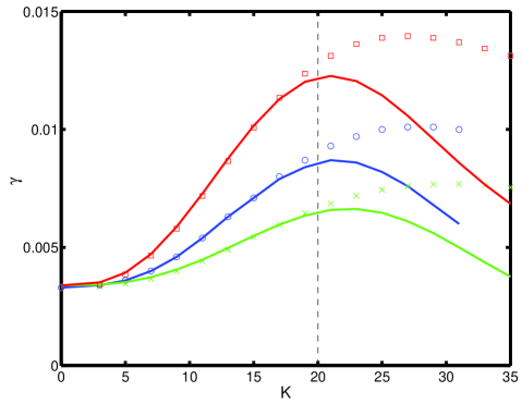
Figure 1: (Color online). Growth rate of the tearing mode as a function of the corrugation wavelength $K$. The solution is obtained for $S=10^{3}$, $\Delta^{\prime}_{0}=0.41$, $\lambda=0.045$ and $\alpha=0$. Crosses, circles and squares represents cases with $A$ equals to $5\times 10^{-5}$, $1\times 10^{-4}$, $2\times 10^{-4}$ respectively. The solid lines show the theoretical prediction for the different cases. The thin vertical line represents the limit of validity of the theoretical prediction ($K\lambda=1$).

In the figure the crosses, circles and squares represent the numerical solutions obtained with the linear code for corrugations of amplitude $5\times 10^{-5}$, $1\times 10^{-4}$, $2\times 10^{-4}$, respectively. When $K<40$ (i.e. $K\lambda<1.82$), these values lead to current corrugations of maximum amplitude smaller than 7%, 15% and 30% of the equilibrium current density. We remark that even small amplitude corrugations can strongly modify the growth rate of the mode. For example, in the case shown here a corrugation that amounts to 4% of the amplitude of the equilibrium current density (e.g. $A=1\times 10^{-4}$ and $K\lambda=0.91$) can lead to a growth rate three times as large than in the ”smooth” case. For values of $K\lambda$ smaller than 1 ($K<20$ in our example), the theoretical predictions obtained from the dispersion relation Eq.15 together with the scaling Eq.12, are in excellent agreement with the numerical data. The disagreement for larger values of the corrugation’s wavelength is due to the limitations of the validity of the scaling. Furthermore, also the dispersion relation Eq.15 is not correct when the constant-$\widetilde{\psi}$ approximation does not hold anymore.

To complement this analysis, we have independently calculated with a different numerical code the value of $\delta\Delta^{\prime}$ associated to the corrugations and the equilibrium described above. The code, that is also used to obtain the cylindrical results presented in the next Section, can solve Eq.4 or its slab version by using a ”shooting” algorithm. As Fig.2 shows, the numerical values of $\delta\Delta^{\prime}$ perfectly match the cubic behavior predicted by the scaling in Eq.12, thus confirming its validity.

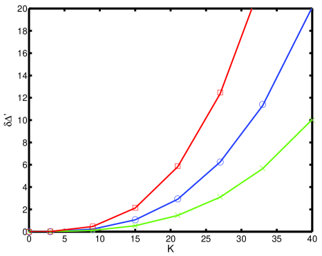
Figure 2: (Color online). $\delta\Delta^{\prime}$ as a function of the corrugation wavelength $K$, for $\Delta^{\prime}_{0}=0.41$ and $\alpha=0$. Crosses, circles and squares represents cases with $A$ equals to $5\times 10^{-5}$, $1\times 10^{-4}$, $2\times 10^{-4}$ respectively. The solid lines show the theoretical prediction (Eq.12) for the different cases.

We complete this study by showing that a current corrugation with the appropriate phase can drive a linear tearing mode even when the ”smooth” equilibrium would assure stability. In Fig.3 we describe three cases, with $\Delta^{\prime}_{0}=0$ (red squares), $\Delta^{\prime}_{0}=-0.29$ (blue circles) and $\Delta^{\prime}_{0}=-0.8$ (green crosses), for a corrugation of amplitude $A=1\times 10^{-4}$.

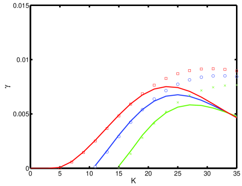
Figure 3: (Color online). Growth rate of the tearing mode as a function of the corrugation wavelength $K$. The solution is obtained for $S=10^{3}$, $A=1\times 10^{-4}$ and $\alpha=0$. Crosses, circles and squares represents cases with $\Delta^{\prime}_{0}$ equals to $-0.8$, $-0.29$ and $0$ respectively. The solid lines show the theoretical prediction for the different cases.

As expected, if the wavelength of the corrugation exceeds a critical threshold, depending on $\Delta_{0}^{\prime}$, the instability can be excited. We conclude remarking that, for $\alpha=0$, the choice of a positive $A$ leads to destabilization, while a negative value would produce the opposite effect.

IV Effect in cylindrical geometry

The analytic results in Section III suggest the possibility that the stability of the tearing mode can be significantly affected by the presence of small scale, small amplitude current corrugations. The scaling that we have obtained is verified by numerical codes in slab geometry, and its validity is confirmed in this Section for cylindrical geometry, which is more relevant for experimental applications. In order to proceed, we perform a numerical study with the ”shooting” code introduced in the previous Section.

We assume a ”rounded” equilibrium current density Furth1973 given by: $J_{eq0}=J_{0}/[1+(r/r_{0})^{4}]^{3/2}$, which implies an equilibrium magnetic flux: $\psi_{eq0}=-0.25J_{0}r_{0}^{2}\sinh^{-1}[(r/r_{0})^{2}]$. Here $J_{0}$ represents the current density at the cylinder axis and $r_{0}$ is a measure of the width of the current channel. In the following we take $J_{0}=2/0.7$ and $r_{0}=\sqrt{1/5}$, so that the mode $m=2$, $n=1$ resonates at $r_{s}\cong 0.73$ and $m=3$, $n=2$ at $r_{s}\cong 0.61$. In our model, the ”zonal” field that generates the current corrugation is sinusoidal and localized around a radius $R$ by a Gaussian envelope of width $\rho$ (taken as $0.2$ in all the simulations): $\delta\psi_{eq}=A\cos[K(r-R)]e^{-(r-R)^{2}/\rho^{2}}$.

We investigate the effect of the corrugation on $m=2$, $n=1$ and $m=3$, $n=2$ modes, which are stable in the ”smooth” configuration since $\Delta^{\prime}_{2,1}\cong-2.19$ and $\Delta^{\prime}_{3,2}\cong-3.28$. We observe that the effect produced by $\delta\psi_{eq}$ on the stability parameter changes as the localization radius of the corrugation is modified and it reaches its maximum when $R\cong r_{s}$ (see Figs.4 and 5).

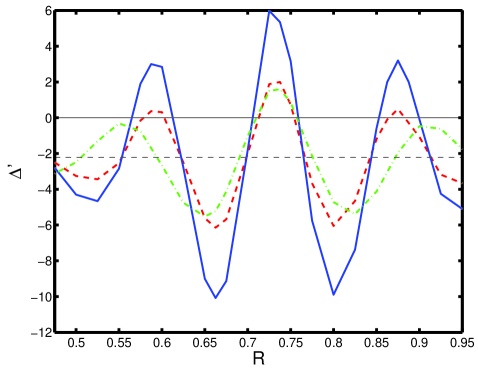
Figure 4: (Color online). $\Delta^{\prime}$ as a function of the localization radius $R$, for the mode $m=2$, $n=1$ and the equilibrium described in the text (for which $\Delta^{\prime}_{2,1}\cong-2.19$). The solid, dashed and dash-dot lines describe cases with $A=5\times 10^{-5}$ and $K=40$, $A=2.5\times 10^{-5}$ and $K=40$, and $A=5\times 10^{-5}$ and $K=30$, respectively.

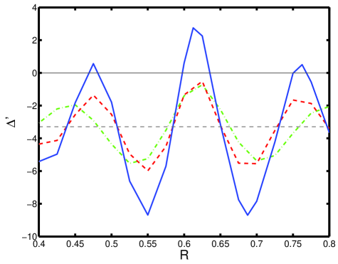
Figure 5: (Color online). $\Delta^{\prime}$ as a function of the localization radius $R$, for the mode $m=3$, $n=2$ and the equilibrium described in the text (for which $\Delta^{\prime}_{3,2}\cong-3.28$). The solid, dashed and dash-dot lines describe cases with $A=5\times 10^{-5}$ and $K=40$, $A=2.5\times 10^{-5}$ and $K=40$, and $A=5\times 10^{-5}$ and $K=30$, respectively.

This is expected, since the rigid shift around the resonance of the sinusoidal perturbation is equivalent to a change in the phase $\alpha$ in in the slab model. Furthermore, the comparison between the solid ($A=5\times 10^{-5}$) and dashed lines ($A=2.5\times 10^{-5}$) in Figs.4 and 5 confirm also in cylindrical geometry the linear dependence of $\delta\Delta^{\prime}$ on the perturbation amplitude, as given in Eq.12. Similarly, also the scaling in the cube of the corrugation wavelength is verified by measuring the maximum amplitude of the solid ($K=40$) and the dash-dot ($K=30$) lines.

Finally, it is interesting to evaluate the constant $C$ for the cylindrical equilibrium investigated. In order to do that, we divide the maximum value of $\delta\Delta^{\prime}$ (obtained at $R=r_{s}$) by the amplitude of the corrugation and the cube of its wavelength. With this procedure we find that $C\cong 2.5$ for $m=2$, $n=1$ and $C\cong 1.7$ for $m=3$, $n=2$. While both values are pretty close to the slab estimate, this result suggest a dependence of the effect of the corrugation on the wave-vector of the driven perturbation. This dependence is easily explained by the presence of the $n/m$ term in the definition of $\psi_{eq0}^{\prime}$ that, in cylindrical geometry, appears in the integral of Eq.10.

V NTM triggering mechanism

In this Section, we analyze how the zonal fields affect the onset of the Neoclassical Tearing Modes. In order to do that, we employ a reduced version of the generalized Rutherford equation Rutherford ; LeHaye2006 ; Itoh2004 :

$$\tau_{\eta}\frac{dw}{dt}\propto\Delta_{0}^{\prime}+\delta\Delta^{\prime}+C_{0}\left(\frac{w}{w^{2}+w_{boot}^{2}}-\frac{ww_{pol}^{2}}{w^{4}+w_{pol}^{4}}\right),$$ (16)

Consistently with Section III, the island width and the stability parameter are normalized to a macroscopic length scale (e.g. the resonant radius). For sake of simplicity, we retain in the model only the fundamental terms responsible for the stabilization/destabilization of the NTM. In particular, we neglect the current shape term, that strongly affects the island saturation but has little effect on the seed island problem Militello2004 ; Escande2004 and the stabilizing toroidal curvature effects Glasser1975 . Furthermore, we do not take into account the rotation of the magnetic island in a self-consistent manner CWW ; Militello2008 . Indeed, in Eq.16 neither the bootstrap term (third on the RHS), nor the polarization term (fourth on the RHS) are explicit functions of the island rotation. The coefficient $w_{boot}$, is a measure of the reduction of the drive associated with the perpendicular transport Fitzpatrick1995 , $w_{pol}$ is the cut-off due to the banana orbit effect Bergmann2002 and $C_{0}$ is a constant proportional to the poloidal $\beta$ LeHaye2006 .

We remark that our purpose is to sketch with an heuristic model the mechanism that could allow NTM formation. A detailed analysis would require a self consistent treatment of Rutherford equation coupled with an equation for the rotation frequency of the magnetic island. The theoretical uncertainties on the exact form of this coupling make an attempt to employ more complicated models to study the problem at hand a futile exercise.

In absence of zonal fields and if $\Delta_{0}^{\prime}<0$, Eq.16 predicts a minimum island width, $w_{seed}$, below which the perturbation is always stabilized and the NTM does not reach macroscopic size. Conversely, when the threshold is exceeded, the dynamical evolution takes the island to its stationary saturation amplitude, $w_{sat}$. To destabilize the NTM an island of sufficient size is therefore required. This ”seed” island could be produced by some other MHD activity in the plasma, such as sawteeth, fishbone instabilities or Edge Localized Modes. In the following we investigate NTM dynamics without a seed [i.e. $w(0)=0$] island but in presence of zonal fields.

From experimental observations Fujisawa2007 ; Fujisawa2008 , we expect that the zonal fields maintain their coherence for a limited amount of time, $\tau_{zf}$. This fact is modelled by assuming a temporal variation of the modified stability parameter, so that $\delta\Delta^{\prime}=\delta\Delta_{max}^{\prime}\cos[(2\pi/\tau_{zf})t]$, where $\delta\Delta_{max}^{\prime}$ is a constant. A critical parameter of the problem is therefore the ratio between this time scale and that typical of the evolution of the NTM. From Eq.16 we infer that this time is a fraction of the local resistive time (calculated with the neoclassical resistivity and the minor radius) $\tau_{NTM}\sim 0.1\tau_{\eta}$, since the saturated island width can be usually estimated around one tenth of $r_{s}$. We expect that rapidly varying zonal fields, such that $\zeta\equiv\tau_{zf}/\tau_{\eta}\ll 1$, will not be an efficient trigger for the NTM as their effect is averaged to zero. On the other hand, if $\tau_{zf}/\tau_{\eta}$ is of the order or greater than one (although the latter possibility is difficult to achieve in fusion plasmas) the zonal fields can drive $w$ above its seed island limit.

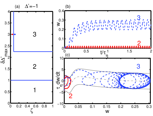
Figure 6: (Color online). NTM triggering mechanism. (a) Approximate boundaries of the relevant solutions of Eq.16, obtained from the numerical solution of Eq.16. Parameters $\delta\Delta^{\prime}$ and $\zeta$ in zone 1 do not produce any island, in zone 2 yield to small ($w<w_{seed}$) oscillating islands, while in zone 3 islands reach full NTM saturation. Physical parameters used described in the text. (b) Time evolution and (c) phase diagram of an island with parameters in zone 2 ($\zeta=0.05$, $\delta\Delta^{\prime}_{max}=2.94$, solid line) and in zone 3 ($\zeta=0.1$, $\delta\Delta^{\prime}_{max}=2.94$, dashed line). The thin solid lines in (c) show $\tau_{\eta}dw/dt$ for the maximum and minimum value of $\delta\Delta^{\prime}$, while the dash-dot line for $\delta\Delta^{\prime}=0$.

The solution of Eq.16 leads to three basic dynamic behaviors for a stable configuration ($\Delta_{0}^{\prime}<0$) in the presence of a corrugation. When $\delta\Delta^{\prime}_{max}<|\Delta^{\prime}|$ the corrugation is not strong enough to produce any island (region $1$ in Fig.6(a)). If the modified stability parameter is sufficiently large, but smaller than a critical value $\delta\Delta_{max}^{{}^{\prime}crit}$, or $\tau_{zf}/\tau_{\eta}<\zeta_{crit}$, an oscillating island appears (region $2$ in Fig.6(a)). Its maximum width remains below $w_{seed}$ and is roughly proportional to $\tau_{zf}$. Finally, when the critical values are exceeded, the full NTM is triggered and the system settles in a state with $w$ oscillating around $w_{sat}$ (region $3$ in Fig.6(a)). The approximate boundaries of these regimes [obtained solving Eq.16 numerically] are sketched in Fig.6(a), for a case with $\Delta^{\prime}=-1$, $C_{0}=0.25$, $w_{boot}=w_{pol}=0.025$, which correspond to reasonable experimental values LeHaye2006 ; Buttery2002 . For clarity, in Fig.6 (b) we show the time evolution of two cases with $\delta\Delta^{\prime}_{max}=2.94$, one just below $\zeta_{crit}$ ( $\zeta=0.05$ for the solid line) and one above ($\zeta=0.1$ for the dashed line). For the same two solutions, we plot in Fig.6 (c) the phase diagram, which describes how $dw/dt$ and $w$ are related during the evolution of the perturbation. Two dots in Fig.6(a) display the position of these cases in the $\delta\Delta^{\prime}_{max}-\zeta$ space.

Obviously, in a realistic situation the time evolution of $\delta\Delta^{\prime}$ would be erratic and Eq.16 would become a stochastic differential equation. We expect that this would make the triggering mechanism easier, with a lower threshold for both the critical $\zeta$ and $\delta\Delta^{\prime}$. An interesting discussion of the stochastic behavior of Rutherford equation was given by Itoh et al. in Ref.Itoh2004 . Furthermore, the calculation presented here is conservative and the critical values obtained are very stringent, since we have assumed an initial condition for Eq.16 with no magnetic island. In reality, the presence of a small, but finite seed island island [$w(0)<w_{seed}$] would move the stability boundaries in Fig.6, broadening the unstable region 3.

VI Conclusions

We have investigated the effect of current corrugations on the stability of the tearing mode. We have obtained a theoretical scaling which relates the change of $\Delta^{\prime}$ to the characteristics of the corrugation, such as its amplitude, typical scale length and phase with respect to the resonant surface. The scaling has been tested on a simple slab linear problem, giving excellent agreement between theoretical predictions and numerical data. Then, by using a shooting code, we have investigated the effect of the corrugations in cylindrical geometry, and found qualitative and quantitative agreement with the analytic scaling. Finally, we have addressed the problem of the seedless trigger of a NTM through a current corrugation.

From our results we conclude that even small modifications of the original equilibrium can lead to significantly different values of the stability parameter and can therefore strongly affect the onset and the dynamics of the mode. For example, a current corrugation of amplitude around $5\%$ of the equilibrium and with scale length comparable with the resistive layer can triple the growth rate of the tearing instability. The study presented in this paper has two clear implications for tokamak experiments.

First, it implies that the calculation of the stability parameters from experimental data is an extremely delicate procedure. Indeed, the current density profiles used to evaluate $\Delta^{\prime}$ cannot be directly measured. While the magnetic field can be deduced from Motional Stark Effect measurements, the best spatial resolution achievable is around 5cm, too coarse to rule out the possibility of current corrugations. Another option is to reconstruct the current profile from temperature and density data by using equilibrium codes. However, the error bars of the measurement and the approximations used in the current reconstruction make it virtually impossible to obtain a precise value of the stability parameter.

The second implication is related to the trigger of the NTMs in a relatively quiescent plasma. Experiments in several machines Gude1999 ; Buttery2002 ; Fredrickson2002 have reported Neoclassical Tearing Modes growing without strong MHD precursors (sawteeth, fishbones or ELMs) which could generate seed islands. The theory presented in this paper suggests the possibility of NTMs triggered by the microscopic turbulence via the generation of slowly evolving (on the NTM time scale) current corrugations. The corrugated configuration could be linearly unstable and generate a seed island, which would then be sustained by Neoclassical physics. At this point, the pressure flattening in the island region could remove the drive for the turbulence and therefore for the zonal field, which would decay, leaving the island at the NTM saturated level. The heuristic model that we have employed shows that a seedless NTM can indeed be excited if the zonal flow that produces the corrugation is sufficiently strong and slowly evolving. Furthermore, even when the zonal field is not able to directly drive the NTM, it can significantly reduce the seed island width (i.e. the plasma becomes more sensitive to the presence of small islands).

It is useful here to give some experimental values for the parameters of our NTM trigger theory. For a typical tokamak plasma, the resistive time is of the order of a few second, hence the islands saturate in roughly 50-100 ms, while the peak frequency for the plasma turbulence is around 100 KHz (as observed for example in Ref.Romanelli2006 ). According to experimental observation of zonal fields by Fujizawa et al. Fujisawa2008 , current corrugations evolve roughly 50 times slower than the drift-wave turbulence. This is in agreement with the theoretical prediction that zonal fields are mesoscale objects. The extrapolation of these results to typical tokamak plasmas leads to an expected coherence time for the corrugations around 1-2 ms. As a consequence, in standard conditions, the value of $\zeta$ is in general below the critical value predicted with our model, which is in agreement with the fact that, in tokamaks, seedless NTMs are the exception rather than the rule. However, current corrugation of sufficient amplitude occurring in particular plasmas (e.g. where the local resistivity is particularly high or the zonal fields are slow) could explain the results in Refs.Gude1999 ; Buttery2002 ; Fredrickson2002 . Furthermore, assuming that the zonal field time scale will be roughly unchanged in the next generation tokamaks, such as ITER, our results seem to suggest that these machines should be stable to spontaneous NTMs, as their resistive time is of the order of hundreds of seconds.

A limitation of this work is the assumption that the pressure profile (and therefore the pressure perturbations) does not play any role in the calculation of $\Delta^{\prime}$. A ”zonal” pressure is generated by drift-waves when Finite Larmor Radius effects are considered and should become significant when ITG instabilities are present. Pressure gradients might be relevant as they contribute to Eq.4 with a term that is inversely proportional to $(\psi_{eq}^{\prime})^{2}$, and are therefore very important in the neighborhood of the resonant surface. As pointed out in Refs.Bishop1991 this could make even harder to properly evaluate the stability parameter. The inclusion of this effect in our calculation will be discussed in a future publication.

The authors acknowledge fruitful discussions with Dr. J.W. Connor, Prof. S.C. Cowley and Dr. A. Thyagaraja. This work was funded by the United Kingdom Engineering and Physical Sciences Research Council and by the European Communities under the contract of Association between EURATOM and UKAEA. The views and opinions expressed herein do not necessarily reflect those of the European Commission.

References

- (1) P.H. Diamond, S-I Itoh, K. Itoh, and T.S. Hahm, Plasma Phys. Control. Fusion 47, R35 (2005).
- (2) A. Fujisawa, K. Itoh, A. Shimizu, H. Nakano, S. Ohshima, H. Iguchi, K. Matsuoka, S. Okamura, T. Minami, Y. Yoshimura, K. Nagaoka, K. Ida, K. Toi, C. Takahashi, M. Kojima, S. Nishimura, M. Isobe, C. Suzuki, T. Akiyama, Y. Nagashima, S.-I. Itoh, and P. H. Diamond, Phys. Rev. Lett. 98, 165001 (2007).
- (3) A. Fujisawa, K. Itoh, A. Shimizu, H. Nakano, S. Ohshima, H. Iguchi, K. Matsuoka, S. Okamura, T. Minami, Y. Yoshimura, K. Nagaoka, K. Ida, K. Toi, C. Takahashi, M. Kojima, S. Nishimura, M. Isobe, C. Suzuki, T. Akiyama, T. Ido, Y. Nagashima, S.-I. Itoh, and P. H. Diamond, Phys. Plasmas 15, 055906 (2008).
- (4) A. Thyagaraja, P.J. Knight, M.R. de Baar, G. M. D. Hogeweij, and E. Min, Phys. Plasmas 12, 090907 (2005).
- (5) R.E. Waltz, J. Candy, F.L. Hinton, C. Estrada-Mila and J.E. Kinsey, Nuclear Fusion 45, 741 (2005).
- (6) B.D. Scott, Private communication (2008).
- (7) H.P. Furth, J. Killeen and M.N. Rosenbluth, Phys. Fluids 6,459 (1963).
- (8) P.H. Rutherford, Phys. Fluids 16, 1903 (1973)
- (9) L.E. Zakharov and A.A. Subbotin, ”Tearing-Mode stabilisation by generation of an additional current layer in Tokamaks”, ITER-IL-Ph11-9-S-2 (available from ITER Secretariat, Max-Plank-Institut für Plasmaphysik, Garching bei München, Germany) (1989).
- (10) E. Westerhof, Nuclear Fusion 30, 1143 (1990)
- (11) J.W. Connor, S.C. Cowley, R.J. Hastie and T.J Martin, Proceedings of the 19th EPS Conference, Innsbruck, 1393 (1992)
- (12) E.A. Adler, R.M. Kulsrud and R.B. White, Phys. Fluids 23, 1375 (1980).
- (13) B. Coppi, J.M. Greene, J.L. Johnson, Nuclear Fusion 6, 101 (1966).
- (14) H.R. Strauss, Phys. Fluids 19, 134 (1976).
- (15) P.N. Guzdar, R.G Kleva and L. Chen, Phys. Plasmas 8, 459 (2001).
- (16) P.N. Guzdar, R.G Kleva, A. Das and P.K. Kaw, Phys. Rev. Lett. 87, 150001 (2001).
- (17) L. Chen, Z. Lin, R.B. White and F. Zonca, Nuclear Fusion 41, 747 (2001).
- (18) F. Militello and F. Porcelli, Phys. Plasmas 11, L13 (2004).
- (19) F. Militello, G. Huysmans, M. Ottaviani and F. Porcelli, Phys. Plasmas 11, 125 (2003).
- (20) D. Grasso, M. Ottaviani and F. Porcelli, Phys. Plasmas 8, 4303 (2001).
- (21) H.P Furth, P.H Rutherford, H. Selberg Phys. Fluids 16, 1054 (1973).
- (22) R.J. La Haye, Phys. Plasmas 13, 055501 (2006).
- (23) S.-I. Itoh, K. Itoh and M. Yagi Plasma Phys. Control. Fusion 46 123-143 (2004).
- (24) F. Militello and F. Porcelli, Phys. Plasmas 11, L13 (2004).
- (25) D.F. Escande and M. Ottaviani, Phys. Lett. A 323, 278 (2004).
- (26) A.H. Glasser, J.M. Greene and J.L. Johnson, Phys. Fluids 18, 875 (1975).
- (27) J.W. Connor, F.L. Waelbroeck and H.R. Wilson, Phys. Plasmas 8, 2835 (2001).
- (28) F. Militello M. Ottaviani and F. Porcelli, Phys. Plasmas 15, 042104 (2008).
- (29) R. Fitzpatrick, Phys. Plasmas 2, 825 (1995).
- (30) A. Bergmann, E. Poli and A.G. Peeters, 19th IAEA Conf. on Fusion Energy (IAEA, Lyon, 2002), paper TH/P1-01.
- (31) A. Gude, S. Günter, S. Sesnic, ASDEX Upgrade Team, Nuclear Fusion 39, 127 (1999).
- (32) R.J. Buttery, T.C. Hender, D.F Howell, R.J. La Haye, O. Sauter, D. Testa and contributors to the EFDA-JETWorkprogramme, Nucl. Fusion 43, 69 (2003).
- (33) E.D. Fredrickson, Phys. Plasmas 9, 548 (2002).
- (34) M. Romanelli, M. De Benedetti, B. Esposito, G. Regnoli, F. Bombarda, C. Bourdelle, D. Frigione, C. Gormezano, E. Giovannozzi, G.T. Hoang, M. Leigheb, M. Marinucci, D. Marocco, C. Mazzotta, C. Sozzi and F. Zonca, Nuclear Fusion 46, 412 (2006).
- (35) C.M. Bishop, J.W. Connor, R.J. Hastie, S.C. Cowley, Plasma Phys. Control. Fusion 33, 389 (1991).