Stochastic Modeling of Single Molecule Michaelis Menten Kinetics

Abstract

We develop an general formalism of single enzyme kinetics in two dimension where substrates diffuse stochastically on a square lattice in presence of disorder. The dynamics of the model could be decoupled effectively to two stochastic processes, (a) the substrate arrives at the enzyme site in intervals which fluctuates in time and (b) the enzymatic reaction takes place at that site stochastically. We argue that distribution of arrival time is a two parameter function specified by the substrate and the disorder densities, and that it correctly reproduce the distribution of turnover time obtained from Monte-Carlo simulations of single enzyme kinetics in two dimension, both in absence and presence of disorder. The decoupled dynamics model is simple to implement and generic enough to describe both normal and anomalous diffusion of substrates. It also suggests that the diffusion of substrates in the single enzyme systems could explain the different distributions of turnover time observed in recent experiments.

I Introduction

Biology of life solely depend on complex chemical reactions brought about by certain specific enzymes. Enzymes are known to facilitate reaction rates without taking part in reactions directlybook . As catalysts, enzymes are receiving increasing importance from other branches of science. The mechanism of enzymatic activity is one of the most fascinating field of physical chemistry. In general in a chemical reactions like ($A+B\rightarrow P$) the rate of reaction depends linearly on the initial concentration of the reactants. But in several enzymatic reactions, where enzyme (or catalyst) $E$ and substrate (or reactant) $S$ form a product $P$, the rate of reaction is known to saturate b with increase of substrate concentration $[S]$ (although the linearity remain valid for low concentration $[S]$), which was explained by Leonor Michaelis and Maud Menten Michaelis in $1913$. In their formulation, it was postulated that enzyme (or catalyst) $E$ and substrate (or reactant) $S$ form a product $P$ through a intermediate enzyme-substrate complex $ES$ as

$${\rm E+S}\mathop{\rightleftharpoons}^{k_{1}}_{k_{2}}{\rm ES}\mathop{\rightarrow}^{k_{3}}E+P$$ (1)

Using law of mass action it was shown that the reaction proceeds with velocity ${{V[S]}\over{([S]+K)}}$, where $V$ and $K$ are constants which depend on the rates of the reaction. Over years this formulation, popularly known as Michaelis-Menten (MM) kinetics, has found applications in different enzymatic reactionsb and in several other systems myxo ; drug . Although Michaelis-Menten kinetic model is based on law of mass action its extension for ordinary or fractal spacial dimesions Sava with or without disorder have been attempted . To incorporate effect of diffusion and noise these multi-enzyme systems have been studied in two dimension using Monte-Carlo simulationBerry .

Recent development of experimental techniques allow one to do single molecule experiments Lu ; Xie , where substrates react stochastically with a single enzyme held at a fixed position. Thus, formation of the products here form a discrete time series, with interspike intervals $\tau$ distributed as $f(\tau)$. It has been shown that the rate of reaction $\langle\tau\rangle^{-1}$ follows MM law independent of the functional form of $f(\tau)$. Thus the distribution of turnover time $f(\tau)$, rather than MM law, could be taken as the characteristic property of any particular single enzymatic reaction system. To understand the variations of $f(\tau)$ observed in experiments several theoretical models Kou ; models have been proposed. In Ref. Kou , density of $S$, $P$, $E$ and $ES$ are replaced by their corresponding probabilities to explain the form of $f(\tau)$. However effect of diffusion and noise, which are known to modify the theoretical description in other low dimensional systemslowD have not been incorporated in these studies.

In this article we study the single enzyme system in two dimension using Monte-Carlo simulation and calculate $f(\tau)$. The substrate molecules $S$, here, are allowed to diffuse on the lattice and react stochastically with the enzyme $E$ fixed at a particular site. We also propose an alternative simple method which illustrate that the dynamics of this two dimensional system which explicitly takes care of the diffusion of the substrates can be decoupled into two separate dynamics; (a) the substrates arrive at the enzyme site in intervals of $\zeta$ which varies stochastically and its distribution is $P(\zeta)$, and (b) the enzymatic reaction (1) takes place at the enzyme site. We further argue that $P(\zeta)$ is a universal two parameter function independent of whether the system has quenched or annealed disorder, or if the diffusion of substrates is normal or anomalous. Given a $P(\zeta)$, the decoupled dynamics can be implemented using a single-site stochastic simulation, which greatly simplify the study by overlooking the full dimensionality of the system.

The article is organized as follows. In section II we describe the Monte-Carlo simulation of single enzyme kinetics in two dimension and calculate the distribution of turnover time $f(\tau)$. Description of the decoupled dynamics, characterization of distribution of substrate arrival time $P(\zeta)$, and comparison of $f(\tau)$ obtained from the decoupled dynamics model with that obtained from Monte-Carlo simulation are discussed in section III. In section IV, we show that the decoupled dynamics model correctly reproduce $f(\tau)$ both in absence and presence of disorder. Finally, in sectionV we conclude the study with some discussions.

II Monte-Carlo simulation of single enzyme kinetics in two dimension

To model the single enzyme kinetics in spacial dimension $d=2$ (SEK2d) we take a $(L\times L)$ square lattice with periodic boundary condition where sites are labeled by two positive integers $(i,j)=1,2,\dots L$. The enzyme is placed at the site $i=L/2=j$, which is denoted as enzyme-site. At very other site, we have a site variable $s_{ij}=0,1,2$ which corresponds to the fact that a site is either vacant, occupied by a substrate $S$ or by a product $P$ respectively. The restriction that each site can be occupied by at most one particle captures the hardcore interactions present among the molecules. The density of the substrates $[S]$ is denoted by $\rho=\frac{N_{S}}{L^{2}}$ where $N_{S}$ is the number of substrates.

The dynamics of the system can be described as follows. Far from the enzyme-site the substrates and the products simply diffuse by making an unbiased move to one of the neighbouring vacant site. These moves are not allowed if all the neighbours are occupied. The enzyme, which is pinned to the enzyme-site, can either be in state $E$ or makes a enzyme substrate complex $ES$. The enzymatic reaction takes place as follows. If the enzyme is in state $E$ and one of the neighbour is occupied by $S$, then $E+S\to ES$ by making the neighbouring site vacant. This process occurs with probability $k_{1}$. Otherwise when $ES$ is present at the enzyme-site and one of the neighbour is vacant, then either reaction $ES\to E+S$ or $ES\to E+P$ occurs with rates $k_{2}$ and $k_{3}$ respectively. The substrate $S$ or the product $P$ which is yield in these reactions goes to the vacant site. Note that, the system is updated in discrete time, hence the probability $k$ that an reaction occurs is same as $rdt$, where $r$ is the rate of that chemical reaction and $dt=1/L^{2}$.

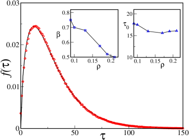
Figure 1: The distribution of turnover time $f(\tau)$ calculated for $\rho=0.1$ is a $\Gamma$-function 2 with $\beta=0.7,\tau_{0}=17.5$.Similar fit could be done for different $\rho$ by taking $\beta$ and $\tau_{0}$ as parameters. The inset shows variation of $\beta$ and $\tau_{0}$ with $\rho$. Other parameters are $k_{1}=1$, $k2=0.001$, $k3=0.03,$ and $L=100$.

To calculate the rate of reaction in a multi-enzyme system one counts the number of products $N_{P}$ in time and then $\frac{dN_{P}}{dt}=-\frac{dN_{S}}{dt}$ gives the rate of reaction. Dependence of the rate on initial substrate concentration $\rho$ is described by the MM law in a regime $\rho\ll 1$. In the single enzyme reaction, however, product forms in discrete intervals $\tau$ whose distribution is defined as $f(\tau)$. To calculate $f(\tau)$ we have done Monte-Carlo simulations of SEK2d and obtain the time interval $\tau$ between formation of any two consecutive products. $\tau$ is measured in units of Monte-Carlo sweep (MCS). As shown in Fig. 1 the distribution of $\tau$ is found to be a $\Gamma$-function,

$$f(\tau)=A\tau^{\beta}\exp(-\tau/\tau_{0}),$$ (2)

where both the exponent $\beta$ and the cut-off scale $\tau_{0}$ depend on density of the substrates $\rho$. The insets of Fig. 1 shows these variations. Note that the distribution $f(\tau)$, shown in Fig. 1, differs substantially from the experimental studies, mainly because, the hardcore interaction here allow only four substrates in the neighbourhood of the enzyme which decreases the turnover probability $f(\tau)$ for small $\tau$. Another possible reason is that the sensitivity of the detector is insufficient in experiments to resolve small turnover time and the observed $f(\tau)$ could be the result of an integrated effect.

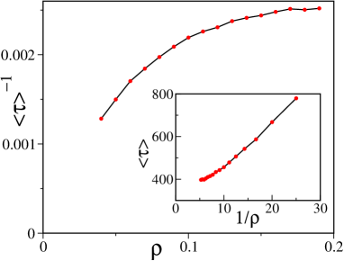
Figure 2: The rate $\langle\tau\rangle^{-1}$ obey Michaelis Menten law. Inset shows that the inverse rate depends linearly on $\rho^{-1}$ for low densities.

Since in single enzyme systems the average time interval between formation of two consecutive products is $\langle\tau\rangle$, the rate of reaction is $\langle\tau\rangle^{-1}$. We have calculated $\langle\tau\rangle^{-1}$ for different $\rho$ and plotted it in Fig. 2. According to MM law inverse rate of turn over depends linearly on the inverse rate of substrate density, which is described in inset of Fig. 2. The linear relation holds good for low densities as expected. Thus, it is evident that this single enzyme system follow MM law independent of the functional form of $f(\tau)$. This has been seen in the experiments of single enzyme systemsXie recently.

However, since the distribution of $\tau$ contains more information than the rate of the reaction $\langle\tau\rangle$ , in this article we give prime importance to $f(\tau)$ and try to achieve a unified formulation which provide a simple method of calculating $f(\tau)$, without doing a two dimensional simulation. This is done in the next section.

III The decoupled dynamics and its stochastic modeling

In the single enzyme systems two different dynamics act separately. First, that the substrates diffuse (with hard core restrictions) through the two dimensional lattice and arrive stochastically at the enzyme site. Second, that the enzymatic reaction (1) takes place there. Based on these decoupled dynamics we introduce a stochastic model of single enzyme kinetics as follows.

In this model, the substrate arrives stochastically at the enzyme site in intervals of $\zeta$ and then the enzymatic reaction takes place there according to (1). For a given distribution $P(\zeta)$, one can simulate this single site dynamics as follows. The enzyme site has two possible states, $E$ and $ES$. If it is in state $E$ it continues to be in the same sate until a substrate $S$ arrives there, and after that it is converted to $ES$ instantly. Otherwise if the site is in state $ES$ it is converted to $E$ stochastically either by forming a product $P$ with rate $k_{3}$ or by breaking the complex $ES\to E+S$ with rate $k_{2}$. However, in the mean time if the substrate arrives while the site is in state $ES$ it falls off. Figure 3 describes this schematically.

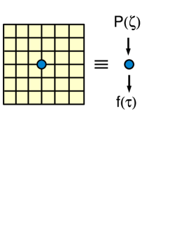
Figure 3: Schematic representation of decoupled dynamics model.

Thus, given $P(\zeta)$ one can calculate $f(\tau)$ numerically using the above stochastic model by noting down the time difference between formation of any two consecutive products. For the simplest model system, where substrates are always available at the enzyme site, $f(\tau)$ can be calculated analytically. In this case, $P(\zeta)=\delta(\zeta-\Delta)$, where $\Delta$ is the unit of time in discrete-time-update (here $\Delta=1~{}MCS$). Thus, the enzyme site is always in the state $ES$ and form products stochastically with with rate $k_{3}$. Of course, $ES$ breaks up with rate $k_{2}$ to from $E+S$, but then instantly $E\to ES$ as other substrates are available at the enzyme site. As expected, this results in an exponential distribution $f(\tau)=A(1-k_{3})^{\tau}$, with $A$ being the normalization constant. The exact form of $f(\tau)$ is compared with that obtained from numerical simulation of decoupled dynamics in Fig. 4.

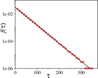
Figure 4: Exact result (solid-line) of the turnover distribution $f(\tau)=A(1-k_{3})^{\tau}$ for $P(\zeta)=\delta(\zeta-1)$ is compared with the corresponding simulation of decoupled dynamics(symbols). Here, $k_{1}=1,k_{2}=0.001,k_{3}=0.03$.

In the next section we calculate $P(\zeta)$ for the single enzyme system.

III.1 Distribution of arrival time $P(\zeta)$

First let us consider the system without hardcore interaction among the substrates, which in turn allows each site of the lattice to accommodate more than one substrate. Hence each substrate in the system does a simple random walk in two dimension. Starting from the enzyme site $E$, a simple random walk would end at a distance within $r$ and $r+dr$ in time $\zeta$ with probability

$$Q(\zeta)=\frac{1}{\sqrt{\pi\zeta}}e^{-r^{2}/\zeta}dr.$$ (3)

Thus, a substrate residing in the region $r$ and $r+dr$ would reach the enzyme $E$ with the same probability $Q(\zeta)$. Therefore the arrival probability of a substrate (from anywhere within the lattice) at $E$ is

$$P(\zeta)=\frac{1}{\sqrt{\pi\zeta}}\int e^{-r^{2}/\zeta}dr\sim C~{}{\rm erf}({A\over\sqrt{\zeta}}),$$ (4)

where $A$ depends on the upper limit of the integral and $C$ is a normalization constant. Note that, for a finite system $\zeta$ can not be larger than a typical time scale $\zeta_{0}$, which introduces a cut-off $\zeta_{0}$ to $P(\zeta)$ ,

$$P(\zeta)=C~{}{\rm erf}({A\over\sqrt{\zeta}})\exp(-{\zeta\over\zeta_{0}}),$$ (5)

Interaction among substrates, e.g. hardcore interaction in our study, further modify Eq. (5) in two ways. It decrease the cutoff $\zeta_{0}$ which now depends strongly on the density of particles $\rho$, and it also modifies the exponet of $\zeta$ which appears in the argument of erf function;

$$P(\zeta)=C~{}{\rm erf}({A\over\zeta^{\alpha}})\exp(-{\zeta\over\zeta_{0}}).$$ (6)

In fact $\alpha$ depends on the exponent $\gamma$ which appears in the mean square displacement of a tagged particle as

$$\langle r^{2}\rangle\sim t^{\gamma}.$$

For non-interacting systems $\gamma=1$, resulting in $\alpha=\gamma/2=1/2$, which is consistant with Eq. (4). In presence of hardcore interaction, however, $\langle r^{2}\rangle$ gets modified by a logarithmic term Henk in the asymptotic regime. Since in the enzymatic systems we are rather interested in the small time limit, the logarithmic term appears as an effective exponent $\gamma^{\prime}>1$ which results in $\alpha>1/2$.

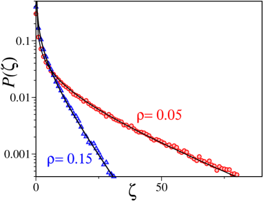
Figure 5: Arrival time distribution $P(\zeta)$ plotted for two different densities $\rho=0.05,0.15$ with $L=100$. The solid lines here corresponds to the best fit according to Eq. (6) with $\alpha=0.64,.7$ , $\zeta_{0}=27.5,7.8$ and $C=1.05,2$ for respective densities. For both the densities $A=0.1$

In the following we calculate $P(\zeta)$ numerically. Substrates, initially placed randomly, are allowed to diffuse on a two dimensional square lattice (with periodic boundary condition). Arrival time of any of the substrates at a pre-decided fixed site is recorded. The distribution $P(\zeta)$ is calculated from the difference between any two consecutive arrival times. The numerical data of $P(\zeta)$ obtained for two different density of substrates $\rho=0.05,0.15$ could be fitted to Eq. (6) by using $\alpha$ and $\zeta_{0}$ as fitting parameters (see Fig. 5). An excellent fit with the numerical data strongly supports the theoretical form of $P(\zeta)$ described by (6).

III.2 Distribution of turnover time $f(\tau)$ for single enzyme system

We have already seen that $f(\tau)$ can be obtained numerically for any given $P(\zeta)$ using the decoupled dynamics model discussed earlier in this section. For the single enzyme problem $P(\zeta)$ is generically described by (6), a function with two parameters $\alpha$ and $\zeta_{0}$ (unless otherwise specified we take $A=0.1$ all through the article). For the same system we know from the Monte-Carlo simulations of single enzyme systems that $f(\tau)$ is a $\Gamma$-function. First let us check that if $P(\zeta)$ given by (6) truly produce the same $\Gamma$-function in the decoupled dynamics model. Figure 6 demonstrates that numerical data for $f(\tau)$ obtained from the decoupled dynamics model fits well with a $\Gamma$-function.

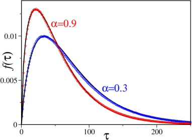
Figure 6: $f(\tau)$ obtained from the decoupled dynamics model is a $\Gamma$-function with $(\beta,\tau_{0})=(.85,40),(0.61,34.5)$ for $(\alpha,\zeta_{0})=(0.3,50),(0.9,50)$ respectively.

Hence from the decoupled dynamics we infer that the parameters of $f(\tau)$ depends on $P(\zeta)$. Thus, for the complete description of the model it is reasonable enough to characterize $(\beta,\tau_{0})$ in terms of $(\alpha,\zeta_{0})$ which is done in the following. Figure 7 shows the dependence of $\beta$ on $\alpha$ for different values of $\zeta_{0}=15,25,50,70,100$. Clearly from the numerical data it emerges that

$$\beta=1-\frac{\alpha}{2}.$$ (7)

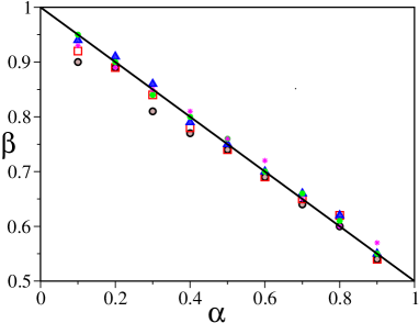
Figure 7: The figure shows $\beta$ versus $\alpha$, calculated form the decoupled dynamics model, for $\zeta_{0}=15,25,50,70$ and $100$ (different symbols). The relation $\beta=1-\alpha/2$ (solid-line) is satisfied for all values of $\zeta_{0}$.

Similarly Fig. 8 describes the dependence of $\tau_{0}$ on $\zeta_{0}$ for different values of $\alpha=0.3,0.5,0.7,0.9$. From the figure it it is clear that $\tau_{0}$ is independent of both $\alpha$ and $\zeta_{0}$ below a specific time scale $\zeta^{*}$. For $\zeta>\zeta^{*}$, however, functional dependence of $\tau_{0}$ on $\zeta_{0}$ varies with choice of $\alpha$. We notice that the time scale $\zeta^{*}$ originates from the product formation rate $k_{3}$ (and do not depend on other rates, like $k_{1}$ or $k_{2}$) as

$$\zeta^{*}\simeq\frac{1}{k}_{3}.$$

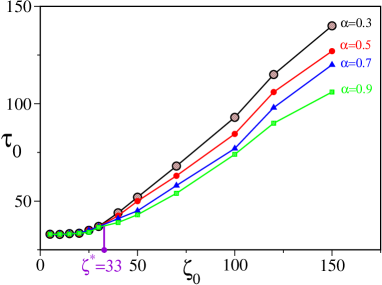
Figure 8: The figure shows $\tau_{0}$ versus $\zeta_{0}$, calculated form the decoupled dynamics model, for different $\alpha$. It is evident that $\tau_{0}$ is independent of $\alpha$ for $\zeta\leq\zeta^{*}$.

Thus, to compare $f(\tau)$ obtained from the two dimensional simulation of single enzyme kinetics with that of the decoupled dynamics model it is convenient to restrict $\zeta_{0}$ in the regime $\zeta_{0}\leq\zeta^{*}=1/k_{3}$. In fact, without loss of generality one may take

$$\zeta_{0}=\zeta^{*}=1/k_{3}.$$ (8)

Otherwise, when $\zeta_{0}>\zeta^{*}=1/k_{3}$, the choice of $\tau_{0}$ would depend explicitly on the value of $\alpha$ (see Fig. 8). A compatible choice, which we use here, is $\zeta_{0}=\tau_{0}$. Thus, to obtain the return time distribution $f(\tau)$ which is characterized by two parameters $\beta$ and $\tau_{0}$ we make a choice of $P(\zeta)$ with parameters

$$\alpha=2(1-\beta) \zeta_{0}=\tau_{0}$$ ; (9)

$${\rm and}~{}~{}k_{3} = 1/\tau_{0}$$ (10)

in the stochastic simulation of decoupled dynamics, where the last line of (10) corresponds to the fact that $k_{3}$ is constrained by (8), and we have used $\zeta_{0}=\tau_{0}$. In the next section we will check if choice (10) in decoupled dynamics model reproduce the $f(\tau)$ same as that of SEK2d.

III.3 Comparison of decoupled dynamics model with Monte-Carlo simulation

From the last section we have seen that the stochastic decoupled dynamics model generates a correct form of $f(\tau)$ for any $P(\zeta)$ given by Eq. (6). To make a correspondence with the SEK2d one needs a mapping between two parameters of $f(\tau)$, namely ($\beta,\tau_{0}$), with ($\alpha,\zeta_{0}$) of $P(\zeta)$. From the numerical characterization of $P(\zeta)$ described in Fig. 7 and 8, we have seen that the mapping is not unique. The same values of ($\beta,\tau_{0}$) can be obtained from different ($\alpha,\zeta_{0}$) by varying the reaction rates of stochastic model. We take an advantage of this situation to make a choice (10). Now let us verify if such choice works.

In Fig. 9 we have compared $f(\tau)$ obtained from single enzyme kinetics in two dimension and corresponding decoupled dynamics model for two different densities $\rho=0.1,0.21$. To calculate $f(\tau)$ for density $\rho=0.1$, which is a $\Gamma$-function with $\beta=0.70$ and $\tau_{0}=17.5$, we simulate the decoupled dynamics for this system with $\alpha=.6,\zeta_{0}=17.5$ and $k_{3}=0.057$ as prescribed by Eq. (10). Similar procedure is used for $\rho=0.21$ where $\beta=0.5$ and $\tau_{0}=16.1$.

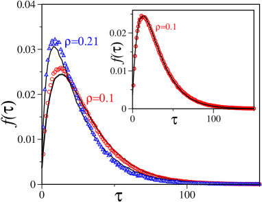
Figure 9: $f(\tau)$ obtained from decoupled dynamics model is compared with the same obtained from SEK2d for two different $\rho=0.1,0.21$. Other parameters are $k_{1}=1,k_{2}=0.001$.

From Fig. 9 it is clear that $f(\tau)$ obtained from SEK2d matches reasonably well with that obtained from corresponding decoupled dynamics. A small discrepancy which is visible for both the densities is possibly due to the fact that a discretized form of $P(\zeta)$ and a cut-off in $\zeta$ has been used in the numerical simulation for convenience. A minor modification of $\zeta_{0}$ can compensate for this discrepancy. $f(\tau)$ with a modified $\zeta_{0}=18.5$ for density $\rho=0.1$ is presented in the inset.

From the above analysis it is evident that the formulation of decoupled dynamics model works well for single enzyme systems without disorder. In the next section we will apply the same formalism to systems with mobile or immobile impurities.

IV Single enzyme systems in presence of disorder

In this section we discuss the effect of disorder in SEK2d. Disorder can be introduced in the single enzyme system by introducing $N_{D}$ impurities in the two dimensional lattice. In case of annealed disorder, the impurities are allowed to diffuse in the system. Thus, it is equivalent to a late time single enzyme system without disorder when products are considered as diffusing impurities. Compared to systems without disorder, here, only the cut-off time scale $\tau_{0}$ is larger. So, in this section we choose to work in the system of quenched disorder in details. The impurities in these systems are immobile and do not diffuse through the system. Thus the substrates are restricted from visiting these impurity sites, and the effective dimension of these system are $d<2$. Simple diffusion on these fractal lattices fractal are anomalous where mean square displacement is given by $\langle r^{2}\rangle\sim t^{\gamma}$ with $\gamma<1$. Note that $\gamma=1$ corresponds to the normal diffusion. Obviously, $\gamma$ depends on the disorder density $\rho_{D}=N_{D}/L^{2}$ for small disorder densities. Beyond a critical density $\rho_{D}>0.4$ Sahimi however the disorder sites percolate and the substrates remain confined in certain islands.

Figure 10: $f(\tau)$ obtained from decoupled dynamics model (solid line) is compared with that of SEK2d (symbols) for disorder density $\rho_{D}=0.1$ and density of substrates $\rho=0.1$. Here $k_{3}=0.03$ for SEK2d and $k_{3}={1\over\tau_{0}}$ for decoupled dynamics model.Other parameters are $k_{1}=1,k_{2}=0.001$.

The anomalous diffusion is expected to change the behavior of arrival time distribution $P(\zeta)$. In particular, if we ignore hardcore interaction among the substrates, Eq. (5) gets modified in presence of disorder as

$$P(\zeta)=C~{}{\rm erf}({A\over\zeta^{\gamma/2}})\exp(-{\zeta\over\zeta_{0}}).$$ (11)

Again, the hardcore interaction introduces a a logarithmic correction term to the mean square displacement, as we have seen in systems without disorder in section III A. This correction may appear in Eq. (5) as an effective exponent $\alpha\neq\gamma/2$. Next, we ask if $f(\tau)$ is still a $\Gamma$-function in presence of quenched disorder, and if the decoupled dynamics with a choice (10) reproduces correct $f(\tau)$. It turns out that answer to both the questions are positive which is described in Fig. 10. To calculate $f(\tau)$ we did a Monte-Carlo simulation of single enzyme kinetics on a two dimensional square lattice ($100\times 100$) with $\rho_{D}=0.1$ and $\rho=0.1$. This gives rise to $f(\tau)$ as given in (2) with $\beta=0.72$ and $\tau_{0}=20$. From Eq. (10) one would then expect that $\alpha=0.57$ and $\zeta_{0}=20$ would generate the same $f(\tau)$ from decoupled dynamics model if $k_{3}=0.05$. Calculated $f(\tau)$ for both the decoupled dynamics model(solid line) and SEK2d (symbols) are shown in Fig. 10. Clearly $f(\tau)$ for the decoupled dynamics model compares well with SEK2d. Note that, as expected, the value of $\alpha=0.57$ in case of disorder is smaller than $\alpha=0.60$ for the system without disorder.

A very good agreement of decoupled dynamics with that of the SEK2d even in presence of quenched disorder suggests that the former stochastic model provide an alternative simple description of single enzyme systems.

V Conclusion

In conclusion we have studied the Monte-Carlo dynamics of single enzyme system in two dimension both in presence and absence of quenched disorder. In both cases the distributions $f(\tau)$ of turnover time $\tau$ are found to be a $\Gamma$-function described by the exponent $\beta$ and the cutoff scale $\tau_{0}$. We argue that the dynamics of the single enzyme system could be decoupled to two stochastic processes; first that the substrates arrive at the enzyme site in intervals which fluctuate in time, and second that the reaction occurs at the enzyme site. We argue that the distribution of substrate arrival time $P(\zeta)$ is a specific function (6) of two parameters $\alpha$ and $\zeta_{0}$. This functional form (5) is generic for systems with or without disorder. By choosing these parameters $\alpha$ and $\zeta_{0}$ according to Eq. (10), we further show that the decoupled dynamics model correctly reproduce $f(\tau)$ obtained from the Monte-Carlo simulation of single enzyme kinetic models defined on a square lattice.

Distribution of turnover time $f(\tau)$, rather than the rate $\langle\tau\rangle^{-1}$, is a characteristic feature of a specific single enzyme system. Following the experiments in these systemsXie several theoretical models have been proposed to explain the underlying cause behind the variation in observed $f(\tau)$. In these formulations, after the enzyme-substrate complex breaks up by forming a product the enzyme returns to its normal state with a delay. Such a delay is considered to be essential Kou , without which asymptotic decay of $f(\tau)$ for large $\tau$ can not be obtained. Further, all the reaction rates there are assumed to vary stochastically, which is attributed to the dynamic disorder associated with several possible conformal variations of enzyme and enzyme-substrate complex. Alternatively, here we show that a simple Michaelis-Menten kinetics (1) in presence of diffusion and noise could produce the same $f(\tau)$ observed in experiments.

References

- (1) Enzymes, M. Dixon and E. C. Webb, Longmans, London (1960).
- (2) S. Albert, E. Will, and D. Gallwitz, The EMBO Jn. 18, 5216(1999); J. S. Reader, and G. F. Joyce, Nature 420, 841(2002); O. Cordin et. al., The EMBO Jnl. 23, 2478(2004); R. V. de Souza et. al., Braz. Arc. Bio. Tech. 48, 105(2005).
- (3) L. Michaelis and M. L. Menten, Biochem. Z. 49, 333(1913).
- (4) M. Watve et al., Curr. Sci. 78, 1535(2000).
- (5) E. M. Rebeccah, A. R. Terence , Phy Rev E 75, 031902(2007).
- (6) M. A. Savageau, J. ther. Biol. 176, 115(1995).
- (7) H. Berry, Biophys. Jnl. 83, 1891(2002).
- (8) H. P. Lu, L. Xun, X. S. Xie, Science 282, 18877(1998).
- (9) B. P.English et. al., Nature Chem. Bio. 2, 87 (2006).
- (10) S. C. Kou, B. J. Cherayil, W. Min B. P. English, and X. S. Xie, J. Phys. Chem. B 109, 19068(2005).
- (11) S. Park, and N. Agmon, J. Phys. Chem. B 112, 5977(2008).
- (12) Diffusion and reaction in fractals and disordered systems, D. ben-Avraham and S. Havlin, Cambridge University Press, Cambridge (2000).
- (13) H. van Beijeren and R. Kutner Phys. Rev. Lett. 55, 238(1985).
- (14) M. J. Saxton, Biophys. Jnl. 66, 394(1994); ibid Biophys. Jnl. 70, 1250(1996); D. S. Banks, and C.Fradin, Biophys. Jnl. 89, 2960(2005).
- (15) M. Sahimi, Appication of Percolation Theory, Taylor & Francis Ltd, London.