New Phase Transitions in Optimal States for Memory Channels
         Vahid Karimipour^† ,         Zohreh Meghdadi^†,          Laleh Memarzadeh^§,

^†Department of Physics, Sharif University of Technology,

11155-9161, Tehran, Iran

^§Dipartimento di Fisica, Universit‘a di Camerino, I-62032 Camerino, Italy.

We investigate the question of optimal input ensembles for memory channels and construct a rather large class of Pauli channels with correlated noise which can be studied analytically with regard to the entanglement of their optimal input ensembles. In a more detailed study of a subclass of these channels, the complete phase diagram of the two-qubit channel, which shows three distinct phases is obtained. While increasing the correlation generally changes the optimal state from separable to maximally entangled states, this is done via an intermediate region where both separable and maximally entangled states are optimal. A more concrete model, based on random rotations of the error operators which mimic the behavior of this subclass of channels is also presented.

PACS Numbers: 03.67.HK, 05.40.Ca

1 Introduction

A basic question in quantum information theory [1, 2, 3, 4, 5] is whether the use of entangled states for encoding classical information can increase the rate of information transmission though a channel or not. A proper calculation of the so called Holevo capacity [3] of a channel, representing by a Completely Positive Trace preserving (CPT) map $\Phi$, requires the optimization of Holevo information over ensemble of input states when we encode information into arbitrary long strings of quantum states (more precisely states in the tensor product of the Hilbert space of one state) and carrying out the limiting procedure $C:=\lim_{n\rightarrow\infty}C_{n}$, where

$$C_{n}:=\frac{1}{n}Sup_{\varepsilon}\chi_{n}(\varepsilon)$$ (1)

is the capacity of the channel, when we send strings of $n$ quantum states into the channel. Here $\varepsilon:=\{p_{i},\rho_{i}\}$ is the ensemble of input states,

$$\chi_{n}(\varepsilon):=S(\sum_{i}p_{i}\Phi(\rho_{i}))-\sum_{i}p_{i}S(\Phi(\rho_{i}))$$ (2)

is the Holevo information of the ensemble and $S(\rho)\equiv-tr(\rho\log\rho)$ is the von Neumann entropy of a state $\rho$. To find the capacity of a given channel we should find the ensemble which maximizes this quantity and we call it the optimal ensemble of input states. Then the properties of this ensemble can be studied and ask whether this ensemble includes entangled states or not.

The importance of this question stems from the fact that entanglement is a vital quantum mechanical resource in many tasks in quantum information processing, however it is a held belief that entanglement is so fragile in the presence of noise. So it would be interesting if one can show by using this property higher rate of data transmission through noisy channels is achievable. The difficulty in answering this question is not only because of the optimization of Holevo information over multi-parameter space but also due to the fact that no concrete classification of multi-particle entangled states exist.

A much simpler problem is to calculate $C_{2}$, rather than $C_{n}$, which is equivalent to refresh the channel after each two uses, and see whether entangled states can enhance Holevo information or not. This problem has been tackled by many authors [6, 7, 8, 9, 10, 11, 12, 13, 14, 15, 16] and for a kind of correlated channel it has been shown that entanglement can enhance the Holevo information, if the correlation is above a certain threshold value. This correlated channel was first introduced in [9] as follows

$$\Phi(\rho)=\sum_{i,j=0}^{3}P_{ij}\sigma_{i}\otimes\sigma_{j}\rho\sigma_{i}\otimes\sigma_{j},$$ (3)

where $\sigma_{i}$, $i=0,1,2,3$ represent Pauli operators $I,\sigma_{x},\sigma_{y}$ , $\sigma_{z}$ and $P_{ij}$, the probabilities of errors $\sigma_{i}\otimes\sigma_{j}$ are correlated in a special way, namely

$$P_{ij}=(1-\mu)p_{i}p_{j}+\mu\delta_{ij}p_{j}.$$ (4)

The parameter $\mu\in[0,1]$, called memory factor signifies the amount of correlation in the noise of the channel. For $\mu=0$, the errors on the two consecutive qubits are completely un-correlated, while for $\mu=1$, the two errors are exactly the same. The idea behind this, is that when the channel relaxation time is much less than the time interval between the passage of the two qubits, the errors will be the same. What was observed in [9] and in subsequent works [12, 14, 16] was that when $\mu$ passes a critical value $\mu_{c}$, the optimal input state jumps suddenly from product states to maximally entangled states.

It is important to note that although the sharp transition of optimal ensemble of input states from product to maximally entangled states is interesting and cause non-analytical behavior of the channel, it is not obvious that the same happens for all kinds of correlated channels. the correlation (4) is one out of many different forms of correlations that one can envisage for a correlated noisy channel. Apart from the mathematical possibility of defining many other forms of correlations, one can also argue on physical grounds, in favor of other forms of correlation. A fully correlated channel which exerts a noise operator on the first qubit, need not exerts the same error operator on the second qubit, as in (4). In fact it is natural to expects that on exerting the first error, the state of the environment will change and depending on this new state, it will exert new errors with conditional probabilities on the second qubit even if the time interval between two consecutive uses of the channel be small.

In this paper we try to shed light on these issues and to provide a basis for studying more examples and extend the study of correlated noisy channels by considering more general forms of correlations. Our study will be along the line of references [9, 12, 14, 16], that is we do not consider a specific model of environment, rather we take the abstract definition of the channel as a CPT linear map, defined by its Kraus decomposition [17]. We start in section 2 with the most general form of the action of a correlated Pauli channel on two qubits, where by two plausible requirements, we will restrict the parameters so that the members of this class can be studied by analytical means. Then we focus on one particular subclass and study in detail the optimal ensemble which maximizes its Holevo information. In this same section we propose a general definition of the correlation parameter, and show that when the correlation of the noise in this channel increases, the optimal ensemble changes from a product ensemble to a maximally entangled one. The phase diagram of the model also shows other interesting transitions not already observed in other works [9, 12, 14, 16]. In fact the phase diagram contains three distinct phases, a product one and two maximally entangled ones, which differ with each other by a relative phase. We also observe that when we consider the correlation parameter and move through this phase diagram, the optimal ensemble changes from product to maximally entangled, however this transition is mediated by a region of correlation, where both maximally entangled and separable ensembles are optimal. Finally we construct a rather concrete model for this particular type of correlation. The paper concludes with a discussion.

2 The correlated action of a Pauli channel on two qubits

The general action of a Pauli channel on two qubits is defined by the following CPT map

$$\Phi(\rho)=\sum_{ij}P_{ij}\sigma_{i}\otimes\sigma_{j}\rho\sigma_{i}\otimes\sigma_{j},$$ (5)

where $P_{ij}$ is the probability of the errors $\sigma_{j}$ and $\sigma_{i}$ on the first and second qubits entering the channel respectively. The number of independent error probabilities are 15 due to normalization $\sum_{i,j}P_{ij}=1$.

In order to see how much correlated the noise on the two consecutive qubits are, we form the marginal error probabilities $p^{(1)}$ and $p^{(2)}$ and evaluate the following distance between the two probability distributions, $p_{ij}$ and $p^{(1)}_{i}p^{(2)}_{j}$, denoted as ${\cal C}$

$${\cal C}:=\frac{1}{2}\sum_{i,j=0}^{3}|P_{ij}-p^{(1)}_{i}p^{(2)}_{j}|$$ (6)

where $p^{(1)}_{i}:=\sum_{j}P_{ij}$ and $p^{(2)}_{i}=\sum_{j}P_{ji}.$ For uncorrelated noise we will have ${\cal C}=0$ and for a fully correlated noise ${\cal C}$ will attain its maximum value. For the probability distribution (4), ${\cal C}$ turns out to be ${\cal C}=\mu\sum_{i=0}^{3}p_{i}(1-p_{i}),$ hence for fixed error probabilities, the correlations indeed increase with $\mu$.

There are two difficulties in studying such a channel for obtaining its optimal input ensemble and understanding how it depends on the correlation of the noise. The first one is that the probability distribution $P_{ij}$ can be correlated in many different ways and picking out a single parameter and designate it as the memory of the channel, is just one possibility. The second problem is that the manifold of input states has itself 6 real parameters which means that the optimization task should be done over a 6 parameter space and thus analytical treatment of such a channel is almost impossible. To overcome these problems, we impose the following symmetry on the channel,

$$\Phi(\sigma_{3}\otimes\sigma_{3}\rho\sigma_{3}\otimes\sigma_{3})=\Phi(\rho).$$ (7)

This is the symmetry which has been considered in [12] for making the model amenable to analytical treatment. Demanding this symmetry reduces the number of parameters in $P_{ij}$ to 7 parameters:

$$P=\left(\begin{array}[]{cccc}p&t&u&s\\ v&q&r&w\\ w&r&q&v\\ s&u&t&p\end{array}\right),$$ (8)

with normalization relation between the parameters. However it is more plausible to assume that the marginal error probabilities on the first and the second qubits be equal, that is

$$p^{(1)}_{i}=p^{(2)}_{i}\hskip 28.45274pt\forall\ i,$$ (9)

Here we are assuming that the errors on a sequence of qubits should be the same, regardless of how we enumerate the qubits of the sequence. What really matters is that any two consecutive uses of the channel are correlated.

This assumptions in addition to the constrained composed by the symmetry in (7 reduce the number of parameters from to 6 and the final form of the matrix of probabilities $P$ with elements can be parameterized as follows:

$$P=\left(\begin{array}[]{cccc}p&\frac{\eta+\xi}{4}&\frac{\eta-\xi}{4}&s\\ \frac{\eta+\gamma}{4}&q&r&\frac{\eta-\gamma}{4}\\ \frac{\eta-\gamma}{4}&r&q&\frac{\eta+\gamma}{4}\\ s&\frac{\eta-\xi}{4}&\frac{\eta+\xi}{4}&p\end{array}\right),$$ (10)

where $p+q+r+\eta+s=\frac{1}{2}.$
The advantage of demanding the symmetry in (7) in not only in reducing the parameters of $P$ but also in reducing the parameters of the general input states.

Following [12], we form the optimal ensemble by finding a state $\rho^{*}$ which minimizes the output entropy and hence minimizing the second term in the right hand side of (2). The input ensemble is then formed as a uniform distribution of the states ${\cal E}=\{\rho_{ij}:=(\sigma_{i}\otimes\sigma_{j})\rho^{*}(\sigma_{i}\otimes\sigma_{j})\}$. The reason is that the first term of the Holevo quantity is maximized by this choise, i.e.

$$S(\sum_{ij}p_{ij}\Phi(\rho_{ij})) = S(\frac{1}{16}\sum_{ij}\sigma_{i}\otimes\sigma_{j}\Phi(\rho^{*})\sigma_{i}\otimes\sigma_{j})$$ (11)

$$= S(\frac{1}{4}I)=2,$$ (12)

where in the first line we have used the covariance property of the channel:

$$\Phi(\sigma_{i}\otimes\sigma_{j}\rho\sigma_{i}\otimes\sigma_{j})=(\sigma_{i}\otimes\sigma_{j})\Phi(\rho)(\sigma_{i}\otimes\sigma_{j}).$$ (13)

and in the second line the Shur’s first lemma for irreducible representations of the Pauli group.

Therefore finding the optimum ensemble of input states reduces to finding a single input state which minimizes the output entropy and we call it optimum input state. Regarding the convexity of entropy we deduce that we should search for the optimal input state among pure states which in general has 6 parameters. However, we are able to restrict the form of the input states to the simple states which are invariant under the above symmetry in (7)

$$|\psi\rangle=\cos\theta|00\rangle+\sin\theta e^{i\phi}|11\rangle,$$ (14)

It is easy to find the output state of this channel with the above form of error probabilities. A straightforward calculation shows that the output state, in the computational basis $\{|00\rangle,|01\rangle,|10\rangle,|11\rangle\}$ will be

$$\Phi(\rho)=\left(\begin{array}[]{cccc}\varepsilon_{00}&0&0&\varepsilon_{03}\\ 0&\varepsilon_{11}&\varepsilon_{12}&0\\ 0&\varepsilon_{12}^{*}&\varepsilon_{22}&0\\ \varepsilon_{03}^{*}&0&0&\varepsilon_{33}\end{array}\right)$$ (15)

where

$$\varepsilon_{00} = 2(p+s)\cos^{2}(\theta)+2(q+r)\sin^{2}(\theta)$$ (16)

$$\varepsilon_{33} = 2(p+s)\sin^{2}(\theta)+2(q+r)\cos^{2}(\theta)$$ (17)

$$\varepsilon_{03} = \sin(2\theta)[(p-s)e^{-i\phi}+(q-r)e^{i\phi}]$$ (18)

$$\varepsilon_{12} = \frac{1}{2}\sin(2\theta)[\xi e^{-i\phi}+\gamma e^{i\phi}]$$ (19)

$$\varepsilon_{11} = \varepsilon_{22}=\eta.$$ (20)

Due to the block diagonal structure of this matrix, its eigenvalues can be calculated in closed form and hence a complete specification of the optimal input states can be made for this general class of correlated Pauli channels.

2.1 Detailed study of a subclass and its phase diagram

As an interesting and simple example, we consider a channel where only the parameters $p$, $q$ and $r$ are non-vanishing, that is matrix of probabilities has the following form

$$P=\left(\begin{array}[]{cccc}p&0&0&0\\ 0&q&r&0\\ 0&r&q&0\\ 0&0&0&p\\ \end{array}\right),$$ (21)

where due to normalization $p+q+r=\frac{1}{2}.$ The action of the Pauli channel on two consecutive qubits will then be:

$$\Phi(\rho) = p\rho+p\sigma_{3}\otimes\sigma_{3}\rho\sigma_{3}\otimes\sigma_{3}+q\sigma_{1}\otimes\sigma_{1}\rho\sigma_{1}\otimes\sigma_{1}+q\sigma_{2}\otimes\sigma_{2}\rho\sigma_{2}\otimes\sigma_{2}$$ (22)

$$+ r\sigma_{1}\otimes\sigma_{2}\rho\sigma_{1}\otimes\sigma_{2}+r\sigma_{2}\otimes\sigma_{1}\rho\sigma_{2}\otimes\sigma_{1}.$$ (23)

The correlation parameter of this channel is found to be

$${\cal C}:=3p-4p^{2}+|(q+r)^{2}-q|+|(q+r)^{2}-r|.$$ (24)

Using (16), the eigenvalues of the output density matrix are

$$\lambda_{1,2}=0,\hskip 28.45274pt\lambda_{3,4}=\frac{1}{2}\left(1\pm\sqrt{1-16[p(q+r)+Y\sin^{2}(2\theta)]}\right),$$ (25)

where

$$Y:=q(r-p)\cos^{2}\phi+r(q-p)\sin^{2}\phi.$$ (26)

For minimization of output entropy which is $S(\Phi(\rho))=-\lambda_{1}\log\lambda_{1}-\lambda_{2}\log\lambda_{2}$, we should maximize the difference between $\lambda_{1}$ and $\lambda_{2}$. This is achieved by minimizing $Y\sin^{2}2\theta$. Therefore if $Y\leq 0$, we should choose $\theta=\frac{\pi}{4}$ and if $Y\geq 0$, we should choose $\theta=0$. Therefore the line $Y=0$ determines the boundary of the maximally entangled ($\theta=\frac{\pi}{4}$) and the product ($\theta=0$) optimal states. This line is determined by the equations $q(r-p)=0$ and $r(q-p)=0$. In the $(q,r)$ plane these two lines are specified by the equations $2q+r=\frac{1}{2}$ and $2r+q=\frac{1}{2}$.

When $\theta=0$, the value of $Y$ is immaterial, however when $\theta=\frac{\pi}{4}$, then the value of $Y$ should be minimized again. In the maximally entangled region, where $\theta=\frac{\pi}{4}$, we should still minimize $Y$. For $q(r-p)\geq r(q-p)$, $Y$ takes its minimum at $\phi=0$, and for $q(r-p)<r(q-p)$ it will take its minimum at $\phi=\frac{\pi}{2}$. Thus the line $q(r-p)=r(q-p)$ ($q=r$) will separate two types of optimal maximally entangled states from each other. The phase diagram is shown in figure (1).

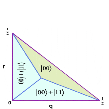
Figure 1: Color Online. The phase diagram of model (14). In each phase the minimum output entropy state (un-normalized) is specified. The triple point is $(q,p)=(\frac{1}{6},\frac{1}{6}).$

It is seen from the phase diagram (2) that as the correlation parameter increases, the optimal input ensemble changes from product to maximally entangled. There are however two remarkable features in this diagram not encountered in previous studies.

First we see that depending on the values of the channel parameters, two different types of maximally entangled states, namely $\frac{1}{\sqrt{2}}(|00\rangle+|11\rangle)$ and $\frac{1}{\sqrt{2}}(|00\rangle+i|11\rangle)$ are optimal. Although these two types of states, are transformed to each other by a local operator $I\otimes\left(\begin{array}[]{cc}1&0\\ 0&i\end{array}\right)$, since the channel is not covariant under this local operator, they should be considered different as far as optimality of the encoding is concerned, although they are equivalent as far as their entanglement properties are concerned [20].

Second, when we draw the contours of constant correlations in this phase diagram, we observed that there is a region of correlation, for which both separable and maximally entangled states are optimal, depending on the values of the parameters $q$ and $r$, figure (2). We say that the two phases coexist, a property which is reminiscent of first-order transitions. We should stress that if one draws the phase diagram of the model in [12], not in terms of the parameter $\mu$, but in terms of the correlation parameter $C$, one will again see such coexistence region. Therefore and specially with regard to recent studies in relating transitions in channel capacity to the critical transitions in their environment [18, 19], it is an interesting issue to see if transitions in the channel should be characterized as first or second order.

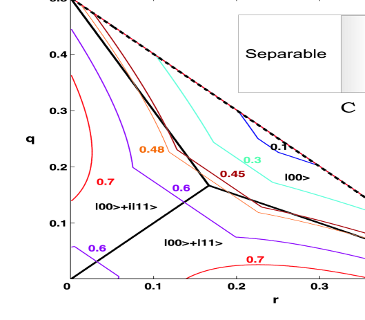
Figure 2: Color Online. The phase diagram of model (14). In each phase the minimum output entropy state (un-normalized) is specified. The contours of constant correlations are also shown. As the correlation ${\cal C}$ increases, the optimal ensemble changes from separable to maximally entangled one. For $\approx 0.43<{\cal C}<\approx 0.5$, both types of states are optimal, the grey region shown in the inset.

2.2 A concrete and intuitive model of correlation

In this section we construct a particular model for correlated noise in Pauli channels, which will reproduce the above example of correlation in a natural way. Consider a noisy Pauli channel acting on a qubit, defined as

$$\Phi(\rho)=\sum_{i=0}^{3}p_{i}\sigma_{i}\rho\sigma_{i},$$ (27)

where $p_{i}$ is the probability of error $\sigma_{i}$ ($\sigma_{0}=I$) and $\sum_{i=0}^{3}p_{i}=1$. When the first qubit passes through the channel, and an error operator $\sigma_{i}$ acts on it, we assume that the state of the channel changes randomly and therefore on the second qubit, it exerts not the same error or a fixed error for that matter, but a random rotation of the $\sigma_{i}$ operator, in the form

$$\tilde{\sigma}_{i}:=U_{{\bf n},\theta}\sigma_{i}U^{\dagger}_{{\bf n},\theta},$$ (28)

where $U_{{\bf n},\theta}$ is a random rotation around the axis ${\bf n}$ with angle $\theta$. Thus $\tilde{\sigma}$ has the effect of the first error operator and also the random change in the environment. This randomness in contrast to a deterministic change in the environment state is physically plausible in view of the macroscopic nature of the environment.

Therefore the action of the channel on two consecutive qubits may be written as follows

$$\Phi(\rho)=p_{0}\rho+\sum_{i=1}^{3}p_{i}\tilde{\sigma}_{i}\otimes\sigma_{i}\ \rho\ \tilde{\sigma}_{i}\otimes\sigma_{i}.$$ (29)

Since the rotations are random, the complete definition of the channel will be given by integrating over the above action with a suitable probability distribution over random rotations. Thus the final definition will be

$$\Phi_{\sigma}(\rho)=\int d{\hat{\bf n}}d\theta P({\bf n},\theta)\Phi(\rho).$$ (30)

Clearly one can add more parameters to the above model, for example by taking different rotations to be along different axes. For simplicity, let us restrict ourself to a simple example in which the direction of all rotations are fixed in the $z$- axis and only the angle of rotation is random. Also to ensure the symmetry (7) we take $p_{0}=p_{3},$ and $p_{1}=p_{2}$, where $p_{0}+p_{1}=\frac{1}{2}$. We take the probability distribution to be a Gaussian with mean value $\theta_{0}$ and variance $\sigma$. Hence the channel will be defined by

$$\Phi_{\sigma}(\rho)=\int\frac{d\theta}{\sigma\sqrt{2\pi}}e^{-\frac{(\theta-\theta_{0})^{2}}{2\sigma^{2}}}\Phi(\rho),$$ (31)

where in this case $\tilde{\sigma}_{i}=e^{-\frac{i}{2}\theta\sigma_{z}}\sigma_{i}e^{\frac{i}{2}\theta\sigma_{z}}$. One can say that parameter $\sigma$ is related to the memory of the channel. When $\sigma=0$, the channel has full memory and it will exert a definite error operator (exactly the same error in the case $\theta_{0}=0$) on the second qubit depending on the operator which it has exerted on the first. However for a non-zero small value of $\sigma$, the channel exerts errors on the second qubit which are close to the errors on the first qubit. As $\sigma$ increases further the memory is lost further and the channel will exert errors from a larger neighborhood of the errors on the first qubit.

A remark is in order about the Gaussian distribution. The rotation operators are periodic which restrict the range of integration of $\theta$ to $[0,2\pi]$. However this makes the subsequent formulas unduly cumbersome without adding much to the physics. Instead we can assume the variance $\sigma$ to be sufficiently less than $2\pi$ so that we can safely extend the range of integration of $\theta$ to $(-\infty,\infty)$ and use the simple results of Gaussian integration.

After rearranging and doing the integrals, one finds that this channel has the form (22) with the parameters as given below

$$p = p_{0},$$ (32)

$$q = p_{1}(\frac{1+e^{-2\sigma^{2}}}{2}),$$ (33)

$$r = p_{1}(\frac{1-e^{-2\sigma^{2}}}{2}),$$ (34)

The two independent parameters of this channel can be taken to be $p_{1}$ and $\sigma$. In terms of these parameters the phase diagram is shown in figure (3). Since we have always $r<q$, the region with $\frac{1}{\sqrt{2}}(|00\rangle+i|11\rangle)$ optimal state is not covered in this new phase diagram. The line which separates the product phase from the maximally entangled phase is now given by (35). Inserting the values of $q$ and $r$ from (33) and (34) in the relation $2r+q=\frac{1}{2}$ and simplifying we obtain

$$e^{-2\sigma^{2}}=3-\frac{1}{p_{1}}.$$ (35)

The phase diagram in figure(2) is re-drawn in terms of the new parameters in figure (3).

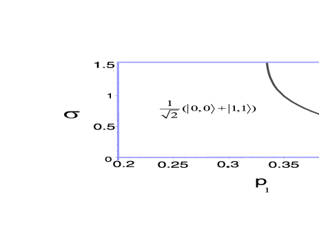
Figure 3: Color Online. The phase diagram of model (24). In each phase the minimum output entropy state is specified.

It is seen that depending on the value of $p_{1}$, the optimal ensemble changes from separable to maximally entangled phase, when the memory passes a certain threshold (note that here a lower value of $\sigma$ means a larger value of memory). Also there are values of $p_{1}$, where the optimal ensemble is always a maximally entangled one, no matter how weak the memory is. This is related to the fact that for no value of the parameter $\sigma$, this channel is a product channel.

As stressed in [16], the effect of memory on the type of optimal ensemble input and ultimately on the capacity of a channel, can be decided only when one considers the action of the channel on arbitrary long sequences of (entangled) qubits. With the type of memory introduced in [9], such extension is very difficult to pursue analytically and one can consider very limited class of states. However with the type of memory introduced above, we think that such an extension is indeed more tractable by analytical means. For example one can consider the following type of correlated action of a Pauli channel on strings of $n$ qubits:

$$\Phi(\rho)=\int dU_{1}dU_{2}\cdots dU_{n-1}\sum_{i=0}^{3}p_{i}\Phi^{(n)}_{i}(\rho)$$ (36)

where

$$\Phi^{(n)}_{i}(\rho)=[\sigma_{i}^{(n-1)}\otimes\cdots\sigma_{i}^{(1)}\otimes\sigma_{i}]\rho[\sigma_{i}^{(n-1)}\otimes\cdots\sigma_{i}^{(1)}\otimes\sigma_{i}]^{\dagger},$$ (37)

and $\sigma_{i}^{(k)}=U_{k}\sigma_{i}U_{k}^{\dagger}$ in which $U_{k}$ is a random unitary operator. Taking the random unitaries from a distribution, one may relate the memory of the channel in a qualitative sense to the properties of the distribution as we did above.

3 Discussion

We have considered a large class of two-qubit correlated Pauli channels for which the entropy of the output state can be determined in closed analytical form. These channels are covariant under the action of the two-qubit Pauli Group and have the symmetry $\Phi(\rho)=\Phi(\sigma_{z}\otimes\sigma_{z}\rho\sigma_{z}\otimes\sigma_{z})$. For a subclass of these channels we have explicitly determined the optimal input ensemble which maximizes the Holevo capacity and have determined the exact phase diagram, showing different regions where separable or maximally entangled states are optimal. There are two new features of this phase diagram. First, there are three phases separable and two different types of maximally entangled states which are optimal. Second if we use a precise definition of correlation, then as the correlation increases the type of optimal state generally changes from separable to maximally entangled states, however this is done through an intermediate region where both separable and maximally entangled states are optimal. Put differently, if we think of correlation as a control parameter, the transition in our model is reminiscent of first order transition where there are regions of coexistence of the two phases. An interesting question is whether such transition occurs when the channel acts upon a string of qubits, not only two consecutive qubits [16]. This is a question which should be addressed if we are to judge definitely wether or not encoding of classical information enhances the classical capacity of quantum channels. Unfortunately settling this question seems to be very difficult.

Finally one would like to see if the transition in the quantum capacity of quantum channels can be related to the well-studied subject of critical phenomena. In this direction a formalism has been developed in [18, 19] where models of correlated noise are constructed by taking a many body system as the environment. The qubits which pass through the channel interact with this many body environment and the correlations in the many body state gives rise to correlations in the noise in the channel. The question of whether the transitions in channel capacity are of first order or not certainly have relevance for such studies.

Acknowledgements We would like to thank S. Alipour, R. Annabestani, S. Baghbanzadeh, M. R. Koochakie, and A. Mani, for valuable discussions. L.M. acknowledges financial support from the EU project CORNER, number FP7-ICT-213681.

References

- [1] M. A. Nielsen, and I. L. Chuang;Quantum computation and quantum information,Cambridge University Press, Cambridge, 2000.
- [2] C.Macchiavello, G.M.Palma and A. Zeilinger, Quantum computation and quantum information theory, World Scientific, Singapore, 2001.
- [3] A. S. Holevo, IEEE Trans. Info. Theory 44, 269-273 (1998).
- [4] B. Schumacher and M. D. Westmoreland, Phys.Rev. A 56, 131-138 (1997).
- [5] P. W. Shor, Equivalence of Additivity Questions in Quantum Information Theory, quant-ph/0305035.
- [6] D. Bruß, L. Faoro, C. Macchiavello, and G.M. Palma, J. Mod. Opt. 47, 325, 2000.
- [7] C. King and M.B. Ruskai, IEEE Trans. Inf. Theory 47,192(2001).
- [8] C. King, Additivity for a class of unital qubit channels, quant-ph/0103156
- [9] C. Macchiavello, and G.M. Palma, Phys. Rev. A 65, 050301(R)(2002).
- [10] K. Matsumoto, T. Shimono and A. Winter, Comm. Math. Phys. 246(3):427-442,(2004).
- [11] K. M. R. Audenaert and S. L. Braunstein, Comm. Math. Phys. (246) No 3, 443-452, (2004).
- [12] Macchiavello, G.M. Palma, S. Virmani, Phys. Rev. A 69, 010303, (2004).
- [13] N.J. Cerf, J. Clavareau, C. Macchiavello. and J. Roland, Phys. Rev. A 72, 042330 (2005).
- [14] V.Karimipour, L.Memarzadeh, Phys. Rev. A 74, 032332, (2006).
- [15] E.Karpov, D.Daems, N.J.Cerf, Phys. Rev. A 74, 032320, (2006).
- [16] V.Karimipour, L.Memarzadeh, Phys. Rev. A 74, 062311, (2006).
- [17] K. Kraus, States, Effects, and Operations: Fundamental Notions of Quantum Theory Springer, Berlin, 1983.
- [18] M.B.Plenio, S.Virmani, Phys. Rev. Lett. 99,120504(2007).
- [19] D.Rossini, V.Giovannetti, S.Montangero, New J.Phys.10, 115009(2008).
- [20] W. D r, G. Vidal, and J. I. Cirac, Phys. Rev. A 62, 062314 (2000).