The Fermi surface and the role of electronic correlations in Sm_2-xCe_xCuO₄

Abstract

Using LDA+GTB (local density approximation+generalized tight-binding) hybrid scheme we investigate the band structure of the electron-doped high-$T_{c}$ material Sm_2-xCe_xCuO₄. Parameters of the minimal tight-binding model for this system (the so-called 3-band Emery model) were obtained within the NMTO ($N$-th order Muffin-Tin orbital) method. Doping evolution of the dispersion and Fermi surface in the presence of electronic correlations was investigated in two regimes of magnetic order: short-range (spin-liquid) and long-range (antiferromagnetic metal). Each regime is characterized by the specific topologies of the Fermi surfaces and we discuss their relation to recent experimental data.

1 Introduction

One of the most important questions in condensed matter is how the strong interaction between quasiparticles modify their properties and influence observable quantities. Non-Fermi-liquid behavior was found in many different substances, but a class of high-$T_{c}$ copper oxides attracts special attention during the last few decades. The unconventional, non-$s$-wave, superconductivity has a lot to do with it. While other players came to stage, like lamellar sodium cobalt oxides and Iron-based pnictide superconductors, only high-$T_{c}$ cuprates combine both strong electronic correlations and high values of critical temperature.

A key issue in a theory of high-$T_{c}$ superconductivity is the proper description of the low-energy electronic structure. Recent experimental results, mainly of angle-resolved photoemission spectroscopy (ARPES) [1, 2, 3] and measurements of quantum oscillations [4, 5, 6], provide a pattern to test various theoretical models and schemes. One of the approaches, proposed by some of the present authors, is the LDA+GTB hybrid scheme [7]. It was shown that the mean-filed theory within this scheme captures the most essential features of the doping-dependent evolution of the quasiparticle band structure and the Fermi surface [8, 9].

A lot of theoretical and experimental efforts were concentrated on the hole doped compounds. Systems with electron doping, Re_2-xCe_xCuO₄ (Re=Nd, Pr, Sm), present a counterpart to hole doped ones and a test for electron-hole asymmetry in Mott-Hubbard insulators. Recent ARPES data on the optimally doped, $x=0.14$, Sm-based compound provide detailed information on the Fermi surface and the band dispersion in the vicinity of the Fermi level [10]. Similar study was reported for Nd-based compound by Schmitt et al. [11]. These results were confirmed independently by the measurement of the quantum oscillations [12]. Also, Park et al. [10] presented an explanation of the observed data based on the $\sqrt{2}\times\sqrt{2}$ spin-density wave (SDW) model. On the other hand, the high-energy electronic structure is found to be inconsistent with the SDW scenario. Moreover, the SDW model implies the weak or moderate electronic correlations and a Fermi liquid background, which is obviously not the case for the underdoped and optimally doped cuprates. Thus it is not a satisfactory scenario and a strong correlation effects should be taken into account.

Here we present the investigation of electronic structure for the electron-doped high-$T_{c}$ material Sm_2-xCe_xCuO₄ by means of LDA+GTB hybrid scheme. Parameters of a minimal generic tight-binding model for these systems (the so-called Emery model) were obtained within the NMTO method. Doping evolution of the band structure and the Fermi surface within this model in presence of strong electronic correlations and magnetic fluctuations were studied in the framework of the GTB method.

The LDA+GTB electronic structure strongly depends on the underlying magnetic order. Though there is no Néel temperature in the optimally doped n-type cuprates, the antiferromagnetic (AFM) correlation length is extremely large ($\lambda\approx 400a$) up to $x=0.17$ [13, 14, 15, 16]. Such correlation length makes magnetic behavior to be rather close to the long-range ordered AFM. That is why our spin-liquid description is unable to capture some details of the observed Fermi surface. On the other hand, there is a good agreement with the recent ARPES data once we assume the presence of the long-range order.

2 Noninteracting band structure

Here we will describe the noninteracting band structure and in the next Section introduce the electronic correlations within the LDA+GTB method.

Sm₂CuO₄ system has body-centered tetragonal crystal structure with the space group $I4/mmm$. Values of lattice parameters are $a=3.917$Åand $c=11.899$Å. The atomic positions for different atoms are: Cu (0,0,0), Sm (0,0,0.35184) and two types of oxygens O1 (0,0.5,0), O2 (0,0.5,0.25) [17]. Physically important CuO₂ layers are constructed with O1 type oxygens. No apical oxygen is presented in this structure.

We perform density functional theory band structure calculations within linear muffin-tin orbital basis set employing atomic sphere approximation in the framework of program package TB-LMTO-ASA v47 [18, 19, 20]. In Fig. 1 results of our LMTO computations are presented. Left panel shows the total and the partial densities of states. Cu-3$d$ and O1-2$p$ states cross the Fermi level. In the right panel of Fig. 1 LMTO band dispersions are presented (thick curves). Note the Fermi level is crossed by just one antibonding hybrid Cu-3$d$—O1-2$p$ band of $x^{2}-y^{2}$ symmetry. It is in agreement with the generic minimal tight-binding model for high-$T_{c}$ cuprates [21, 22]. Orbital basis for this model consists of Cu-$3d_{x^{2}-y^{2}}$ orbital and in-plane $p_{x}$ and $p_{y}$ oxygen orbitals. To compute corresponding model parameters $N$-th order Muffin-Tin orbital method (NMTO) [23] was used. Necessary for NMTO expansion energies are schematically shown on the right side of Fig. 1. Obtained hopping parameters are listed in the Table 1, and the single electron energies are E${}_{x^{2}-y^{2}}=-2.322$ eV and E${}_{p_{x}}=-3.708$ eV.

We assume that the values of Coulomb repulsion $U$ and Hund’s exchange $J_{H}$ for Cu ions are doping independent and equal to 10 eV and 1 eV, respectively (see Ref. [7] for details).

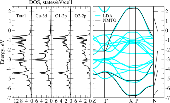
Figure 1: Electronic structure of Sm₂CuO₄ obtained within LDA. Left panel presents total and partial densities of states; right panel shows band dispersions: thick (cyan) curves denote LMTO bands, while thin (black) curves denote NMTO bands. Zero corresponds to the Fermi level.

Table 1: Parameters for the 3-band model obtained within NMTO method. Here $x^{2}$ and $p_{x,y}$ denote the Cu-$3d_{x^{2}-y^{2}}$ and O-$p_{x,y}$ orbital indexes. All values are in eV.

• hopping	involved orbitals
  	($x^{2}$,$p_{x}$)		($x^{2}$,$x^{2}$)		($p_{x}$,$p_{y}$)
  	direction	value	direction	value	direction	value
  t	(0.5,0)	1.261	(1,0)	0.138	(0.5,0.5)	0.882
  t′	(0.5,1)	-0.011	(1,1)	-0.025	(1.5,0.5)	0.033
  t′′	(1.5,0)	0.1	(2,0)	0.011	(1.5,1.5)	0.021
  t′′′	(1.5,1)	-0.007	(1,2)	-0.012	(2.5,0.5)	0.005

3 LDA+GTB scheme

Within the LDA+GTB method [7] the results of ab initio band structure calculations presented in the previous Section are used to construct the Wannier functions and to obtain the parameters of the multiband Hubbard-type model. For this multiband model the electronic structure in the strong correlation regime is calculated within the generalized tight-binding (GTB) method [24, 25, 26]. The latter combines the exact diagonalization of the model Hamiltonian for a small cluster (unit cell) with perturbative treatment of the intercluster hopping and interactions. After this step we end up with the GTB Hamiltonian. Depending on the order of perturbative treatment, we can formulate different approximations.

As was shown before [7], for undoped and weakly doped La_2-xSr_xCuO₄ and Nd_2-xCe_xCuO₄ this scheme in the lowest order in hopping (Hubbard-I approximation) results in a charge transfer insulator with a correct value of the gap $E_{ct}$ and the dispersion of bands in agreement with the experimental ARPES data.

We map the GTB Hamiltonian onto the effective $t-t^{\prime}-t^{\prime\prime}-J^{*}$ model, where “$*$” denotes the three-site correlated hoppings, and study two regimes of AFM correlations. Namely, the spin-liquid phase with short-range AFM fluctuations and the long-range AFM metallic phase. We will describe AFM metallic phase using the Hubbard-I approximation that was shown to be in qualitative agreement with the Quantum Monte-Carlo results [27]. To study the spin-liquid phase, we use the same procedure as in Ref. [8] and go beyond the Hubbard-I approximation: (i) We solve the Dyson equation in the paramagnetic phase by means of the diagram technique for the Hubbard $X$-operators [28] and (ii) Obtain the coupled equations for the self-energy $\hat{\Sigma}(\mathbf{k},\omega)$, the strength operator $\hat{P}(\mathbf{k},\omega)$, and the spin-spin and kinematic correlation functions, (iii) We solve the coupled equations self-consistently and obtain a doping dependent Fermi surface and band structure.

The $t-t^{\prime}-t^{\prime\prime}-J^{*}$ model Hamiltonian is given by

$$H_{t-J^{*}} = H_{t-J}+H_{(3)},$$ (1)

$$H_{t-J} = \sum\limits_{f,\sigma}(\varepsilon-\mu)X_{f}^{\sigma\sigma}+\sum\limits_{f\neq g,\sigma}t_{fg}X_{f}^{\sigma 0}X_{g}^{0\sigma}+\sum\limits_{f\neq g}{J_{fg}\left({\mathbf{S}_{f}\cdot\mathbf{S}_{g}-\frac{1}{4}n_{f}n_{g}}\right)}$$

$$H_{(3)} = \sum\limits_{f\neq m\neq g,\sigma}{\frac{\tilde{t}_{fm}\tilde{t}_{mg}}{U}\left({X_{f}^{\sigma 0}X_{m}^{\bar{\sigma}\sigma}X_{g}^{0\bar{\sigma}}-X_{f}^{\sigma 0}X_{m}^{\bar{\sigma}\bar{\sigma}}X_{g}^{0\sigma}}\right)},$$

where $X_{f}^{nn^{\prime}}\equiv\left|n\right>\left<n^{\prime}\right|$ are the Hubbard $X$-operators [29] acting on the Hilbert space of local states $\left|n\right>=\left\{0,\sigma,-\sigma\equiv\bar{\sigma}\right\}$, $J_{fg}=2\tilde{t}_{fg}^{2}/U$ is the AFM exchange between two sites $f$ and $g$, $U=E_{ct}$ is the effective Hubbard repulsion determined by the charge transfer energy $E_{ct}\approx 2$eV, $t_{\mathbf{k}}=2t(\cos{k_{x}}+\cos{k_{y}})+4t^{\prime}\cos{k_{x}}\cos{k_{y}}+2t^{\prime\prime}(\cos{2k_{x}}+\cos{2k_{y}})$ is the Fourier transform of the hopping $t_{fg}$, and $\tilde{t}_{\mathbf{k}}=2\tilde{t}(\cos{k_{x}}+\cos{k_{y}})+4\tilde{t}^{\prime}\cos{k_{x}}\cos{k_{y}}+2\tilde{t}^{\prime\prime}(\cos{2k_{x}}+\cos{2k_{y}})$ is the Fourier transform of the interband hopping parameter $\tilde{t}_{fg}$, $\mathbf{S}_{f}$ is the spin operator, $\varepsilon$ is the one-hole local energy, and $\mu$ is the chemical potential. The Green function in terms of the Hubbard $X$-operators is

$$G_{\sigma}(\mathbf{k},\omega)=\left\langle\left\langle\left.X_{\mathbf{k}}^{0\sigma}\right|X_{\mathbf{k}}^{\sigma 0}\right\rangle\right\rangle_{\omega}=\frac{(1+x)/2}{\omega-\varepsilon_{0}+\mu-\frac{1+x}{2}t_{\mathbf{k}}-\frac{1-x^{2}}{4}\frac{\tilde{t}_{\mathbf{k}}^{2}}{U}-\Sigma(\mathbf{k})}.$$ (2)

Within our approximations [8], the strength operator $\hat{P}(\vec{k},E)$ is replaced by the occupation factor $(1+x)/2$ and the self-energy $\hat{\Sigma}(\mathbf{k},\omega)$ is frequency independent but preserve momentum dependence,

$$\Sigma(\mathbf{k}) = \frac{2}{1+x}\frac{1}{N}\sum\limits_{\mathbf{q}}\left\{\left[t_{\mathbf{q}}-\frac{1-x}{2}J_{\mathbf{k}-\mathbf{q}}-x\frac{\tilde{t}_{\mathbf{q}}^{2}}{U}-(1+x)\frac{\tilde{t}_{\mathbf{k}}\tilde{t}_{\mathbf{q}}}{U}\right]K_{\mathbf{q}}\right.$$ (3)

$$+ \left.\left[t_{\mathbf{k}-\mathbf{q}}-\frac{1-x}{2}\left(J_{\mathbf{q}}-\frac{\tilde{t}_{\mathbf{k}-\mathbf{q}}^{2}}{U}\right)-(1+x)\frac{\tilde{t}_{\mathbf{k}}\tilde{t}_{\mathbf{k}-\mathbf{q}}}{U}\right]\cdot\frac{3}{2}C_{\mathbf{q}}\right\}.$$ (4)

The spin-spin $C_{\textbf{q}}$ and kinematic $K_{\textbf{q}}$ correlation functions play significant role representing the short-range AFM fluctuations and the kinetic energy reduced by the correlation effects, respectively:

$$C_{\mathbf{q}} = \sum\limits_{\mathbf{f}-\mathbf{g}}e^{-\mathrm{i}(\mathbf{f}-\mathbf{g})\mathbf{q}}\left\langle X_{\mathbf{f}}^{\sigma\bar{\sigma}}X_{\mathbf{g}}^{\bar{\sigma}\sigma}\right\rangle=2\sum\limits_{\mathbf{f}-\mathbf{g}}e^{-\mathrm{i}(\mathbf{f}-\mathbf{g})\mathbf{q}}\left\langle S_{\mathbf{f}}^{z}S_{\mathbf{g}}^{z}\right\rangle,$$

$$K_{\mathbf{q}} = \sum\limits_{\mathbf{f}-\mathbf{g}}e^{-\mathrm{i}(\mathbf{f}-\mathbf{g})\mathbf{q}}\left\langle X_{\mathbf{f}}^{\sigma 0}X_{\mathbf{g}}^{0\sigma}\right\rangle.$$ (5)

Energy spectrum is determined by the poles of the Green function (2) and Fermi surface is determined by the equation $\varepsilon_{0}-\mu+\frac{1+x}{2}t_{\mathbf{k}}+\frac{1-x^{2}}{4}\frac{\tilde{t}_{\mathbf{k}}^{2}}{U}+\Sigma(\mathbf{k})$ = 0.

4 Results and discussion

The procedure of mapping the GTB Hamiltonian onto the effective model was described in detail in Ref. [7]. Following the same steps and using the parameters listed in Table 1, we obtain the $t-t^{\prime}-t^{\prime\prime}-J^{*}$ model with the following hoppings and exchange interactions: $t=-0.59$ eV, $t^{\prime}=-0.08t$, $t^{\prime\prime}=0.15t$, $J=0.92|t|$, $J^{\prime}=0.01|t|$, $J^{\prime\prime}=0.02|t|$, $\tilde{t}=-0.74$ eV, $\tilde{t}^{\prime}=-0.11\tilde{t}$, $\tilde{t}^{\prime\prime}=0.16\tilde{t}$. Here, $\tilde{t}$, $\tilde{t}^{\prime}$, and $\tilde{t}^{\prime\prime}$ are the interband hoppings through the charge-transfer gap, which determine the three-site hoppings and the exchange parameter, $J=2\tilde{t}^{2}/E_{ct}$. Note that although the value of the nearest-neighbor exchange $J$ is quite large, the spin gap in the AFM phase will be determined not by this value alone, also there will be a contribution from the three-site hoppings. This contribution reduce the value of the spin gap as will be discussed later.

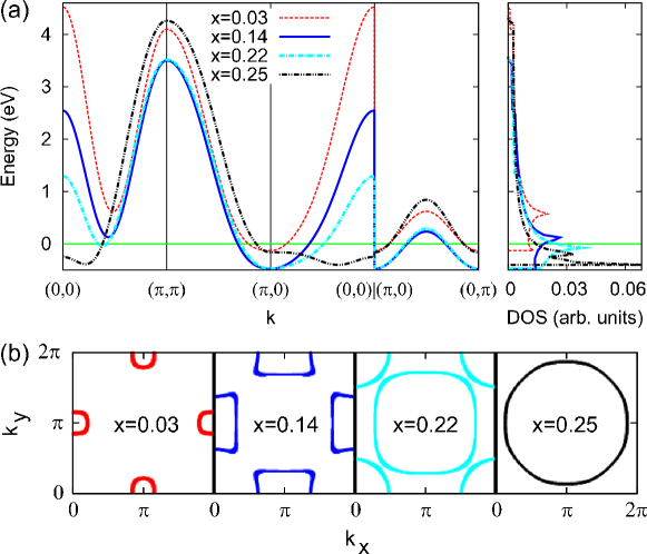
Figure 2: Spin-liquid phase: Band structure and DOS (a) and the Fermi surface (b) for Sm_2-xCe_xCuO₄ within LDA+GTB method for different doping concentrations $x$, as indicated. In (a) zero corresponds to the Fermi level.

In Fig. 2 we present results for $t-t^{\prime}-t^{\prime\prime}-J^{*}$ model in the spin-liquid phase. At low doping, $x=0.03$, due to the scattering on the magnetic fluctuations, the band structure possess local AFM symmetry in the vicinity of the $(\pm\pi/2,\pm\pi/2)$ points [see Fig. 2(a)] and the Fermi surface has a form of four electron pockets around the $(0,\pm\pi)$ and $(\pm\pi,0)$ points. Values of the spin-spin correlation functions $C_{\textbf{q}}$ are large enough for the similar topology to survive until $x\approx 0.22$, where a quantum phase transition with change of the Fermi surface topology takes place. After the transition, the Fermi surface at $x=0.22$ has a form of a large hole pocket around the $(\pi,\pi)$ point and a small hole pocket around the $(0,0)$ point, which decrease in size with further electron doping. At $x=0.25$ only one large hole pocket around the $(\pi,\pi)$ point is left. The quantum phase transition with the change of the Fermi surface topology was found experimentally in Nd-based compound [12], though at a different critical concentration.

Note that the standard formulation of the Luttinger theorem does not work for the Hubbard fermions since the spectral weight of such fermion is determined by the strength operator, $\hat{P}(\textbf{k},E)=F_{0\sigma}$, and each quantum state contains $2F_{0\sigma}=1-x$ electrons. A generalized Luttinger theorem for the strongly correlated systems [32] takes into account the spectral weight of each $\left|k\right\rangle$ state and the Fermi surface in our Fig. 2 satisfies its completely.

A comparison of the calculated Fermi surface in the spin-liquid phase and the experimental ARPES data [10] is shown in Fig. 3. Note the difference in the methods to obtain the Fermi surface “mapping”. We draw a set of constant energy cuts from the Fermi level down to -0.3 eV below it, while the experimental Fermi surface mapping is an integration of ARPES intensities over 30 meV energy window. The ARPES Fermi surface consists of three parts: two pockets around $(0,\pi)$ and $(\pi,0)$ points, and one elongated pocket around $(\pi/2,\pi/2)$ point. One can immediately notice from Fig. 2(b) that in our spin-liquid theory the pocket around $(\pi/2,\pi/2)$ point is missing; it does not appear even if one collects intensities from below the Fermi level, as seen in Fig. 3. Moreover, there are no features in the band dispersion, which could produce such pocket. Thus we conclude that our theory for the spin-liquid phase does not reproduce all details of the experimental Fermi surface.

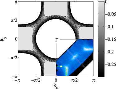
Figure 3: Fermi surface “mapping” (set of equipotential cuts from the Fermi level to -0.3 eV below it) in the spin-liquid phase for $x=0.14$ together with the reproduction of experimental ARPES data from Ref. [10] in the lower right corner. Colorbar on the right shows the correspondence between shades of gray and energy from the Fermi level (in eV).

Since optimally doped Sm_2-xCe_xCuO₄ is in the vicinity of the ordered AFM phase and the correlation length is extremely large (about 400 lattice constants) [16], we now investigate the band structure in the $t-t^{\prime}-t^{\prime\prime}-J^{*}$ model assuming the long-range AFM order. The procedure is similar to Refs. [30, 31], where the energy spectrum of the $t-t^{\prime}-t^{\prime\prime}-J$ model was obtained within the Hubbard-I approximation, but here we also take the three-site hopping terms into account.

In Fig. 4(b) we present results for the Fermi surface in the AFM phase of the $t-t^{\prime}-t^{\prime\prime}-J^{*}$ model at $x=0.14$ together with the experimental ARPES data. Evidently, there is a rather good agreement between both. We would like to mention that for lower concentrations our calculations result in decrease of pockets around the $(\pi/2,\pi/2)$ points and increase of pockets around the $(\pi,0)$ and $(0,\pi)$ points. Note that in the $t-J$ model the spin gap is determined solely by the AFM exchange $J$ [30]. Here, momentum dependence of the spin gap is proportional to $t^{\prime}\cos{k_{x}}\cos{k_{y}}$ (see Eq. (12) of Ref. [30]). The reason is that in the absence of spin fluctuations the hoping of a particle without spin flip processes possible only within the same spin sublattice. Because of the $\cos{k_{x}}\cos{k_{y}}$ functional form the spin gap is maximal at $(\pi/2,\pi/2)$ point and minimal at $(\pi,0)$ point as seen in Fig. 4(a). Since the three-site hopping terms involving sites $f$, $m$, and $g$ are proportional to $\tilde{t}_{fm}\tilde{t}_{mg}/E_{ct}$, they also contribute to the spin gap; but, apparently, they decrease the gap value around $(\pi,0)$ point making it more anisotropic.

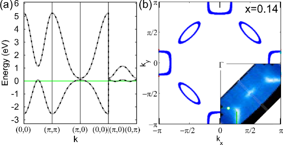
Figure 4: AFM phase: Band structure (a) and the Fermi surface (b) for $x=0.14$ within LDA+GTB method. In the lower right corner of (b) we show the reproduction of the ARPES Fermi surface map from Ref. [10]. In (a) zero corresponds to the Fermi level.

Since we are making a mean-filed theory (though in a strong interaction limit) we can not address the question of the intensity distribution over the Fermi surface. This question was addressed earlier by different groups [33, 34]. Remarkably, their results on the Fermi surface contours for $x\approx 0.14$ are very similar to our’s in Fig. 4 in spite of rather different calculation schemes. This again emphasizes the fact that the AFM correlations are very strong in the optimally electron doped cuprates and they determine the quasiparticle dispersion and the Fermi surface.

5 Conclusion

We have shown that the experimentally observed Fermi surface topology can be explained within the LDA+GTB calculations for the long-range AFM spin background. On the other hand, our theory for the spin-liquid phase demonstrates only partial agreement with the ARPES Fermi surface due to the underestimation of the impact of magnetic scattering on the electronic structure. We conclude that the spin fluctuations are very strong in Sm_1.86Ce_0.14CuO₄ and are closer to the long-range AFM fluctuations rather than to the fluctuations in the spin-liquid phase. Similar conclusion was drawn recently from the analysis of quantum oscillations in Nd-based electron doped cuprates [12].

We would like to emphasize the significant difference between our picture for AFM order and one by Park et al. [10]. Park et al. provide a simple calculation based on the conventional SDW order i.e. the one based on a weak coupling approximation for the interaction. In the absence of the long-range order the ground state is metallic even at zero doping, $x=0$. On the other hand, our approach allows to study the limit of large interaction and provides an insulating ground state at zero doping. This is essential difference since the underdoped cuprates belong to a class of strongly interacting systems and exhibit a Mott transition at a half filling, $x=0$. More precisely, because of the copper-oxygen hybridization the cuprates shows the charge-transfer gap $E_{ct}$ at $x=0$, but on the level of a single-band Hubbard model one can speak about a Mott-Hubbard effective gap $U=E_{ct}$.

References

References

- [1] Yoshida T, Zhou X J, Sasagawa T, Yang W L, Bogdanov P V, Lanzara A, Hussain Z, Mizokawa T, Fujimori A, Eisaki H, Shen Z-X, Kakeshita T, Uchida S 2003 Phys. Rev. Lett. 91 027001
- [2] Damascelli A, Hussain Z, Shen Z-X 2003 Rev. Mod. Phys. 75 473
- [3] Meng J, Liu G, Zhang W, Zhao L, Liu H, Jia X, Mu D, Liu S, Dong X, Lu W, Wang G, Zhou Y, Zhu Y, Wang X, Xu Z, Chen C, Zhou X J 2009 Nature 462 335
- [4] Doiron-Leyraud N, Proust C, LeBoeuf D, Levallois J, Bonnemaison J-B, Liang R, Bonn D A, Hardy W N, Taillefer L 2007 Nature 447 565
- [5] Yelland E A, Singleton J, Mielke C H, Harrison N, Balakirev F F, Dabrowski B, Cooper J R 2008 Phys. Rev. Lett. 100 047003
- [6] Sebastian S E, Harrison N, Palm E, Murphy T P, Mielke C H, Liang R, Bonn D A, Hardy W N, Lonzarich G G 2008 Nature 454 200
- [7] Korshunov M M, Gavrichkov V A, Ovchinnikov S G, Nekrasov I A, Pchelkina Z V, Anisimov V I 2005 Phys. Rev. B 72 165104
- [8] Korshunov M M, Ovchinnikov S G 2007 Eur. Phys. J. B 57 271
- [9] Korshunov M M, Gavrichkov V A, Ovchinnikov S G, Nekrasov I A, Kokorina E E, Pchelkina Z V 2007 J. Phys.: Condens. Matter 19 486203
- [10] Park S R, Roh Y S, Yoon Y K, Leem C S, Kim J H, Kim B J, Koh H, Eisaki H, Armitage N P, Kim C 2007 Phys. Rev. B 75 060501(R)
- [11] Schmitt F, Lee W S, Lu D-H, Meevasana W, Motoyama E, Greven M, Shen Z-X 2008 Phys. Rev. B 78 100505(R)
- [12] Helm T, Kartsovnik M V, Bartkowiak M, Bittner N, Lambacher M, Erb A, Wosnitza J, Gross R 2009 Phys. Rev. Lett. 103 157002
- [13] Sumarlin I W, Skanthakumar S, Lynn J W, Peng J L, Li Z Y, Jiang W, Greene R L 1992 Phys. Rev. Lett. 68 2228
- [14] Gukasov A G, Polyakov V A, Zobkalo I A, Petitgrand D, Bourges P, Boudaréne L, Barilo S N, Zhigunov D N 1995 Sol. State. Commun. 95 533
- [15] Chang B C, Hsu Y Y, Ku H C 2002 Physica B 312-313 59
- [16] Motoyama E M, Yu G, Vishik I M, Vajk O P, Mang P K, Greven M 2007 Nature 445 186
- [17] Takeda H, Okuno M, Ohgaki M, Yamashita K, Matsumoto T 2000 J. Mater. Res. 15 1905
- [18] Andersen O K , Phys. Rev. B 12, 3060 (1975).
- [19] Gunnarsson O, Jepsen O, Andersen O K 1983 Phys. Rev. B 27 7144
- [20] Andersen O K, Jepsen O 1984 Phys. Rev. Lett. 53 2571
- [21] Emery V J 1987 Phys. Rev. Lett. 58 2794
- [22] Varma C M, Schmitt-Rink S, Abrahams E 1987 Solid State Commun. 62 681
- [23] Andersen O K, Saha-Dasgupta T 2000 Phys. Rev. B 62 16219(R)
- [24] Ovchinnikov S G, Sandalov I S 1989 Physica C 161 607
- [25] Gavrichkov V A, Ovchinnikov S G, Borisov A A, Goryachev E G 2000 Zh. Eksp. Teor. Fiz. 118 422 [2000 JETP 91 369].
- [26] Gavrichkov V A, Borisov A A, Ovchinnikov S G 2001 Phys. Rev. B 64 235124
- [27] Ovchinnikov S G, Shneyder E I 2003 Central European J. Phys. 3 421
- [28] Ovchinnikov S G, Val’kov V V 2004 Hubbard Operators in the Theory of Strongly Correlated Electrons (Imperial College Press, London-Singapore)
- [29] Hubbard J C 1964 Proc. Roy. Soc. London A 277 237
- [30] Ovchinnikov S G, Borisov A A, Gavrichkov V A, Korshunov M M 2004 J. Phys.: Condens. Mater 16 L93
- [31] Ovchinnikov S G, Korshunov M M, Zakharova E V 2008 Fiz. Tverd. Tela 50 1349 [2008 Phys. Sol. State 50 1401].
- [32] Korshunov M M, Ovchinnikov S G 2003 Fiz. Tverd. Tela 45 1351 [2003 Phys. Sol. St. 45 1415].
- [33] Aichhorn M, Arrigoni E, Potthoff M, Hanke W 2006 Phys. Rev. B 74 024508.
- [34] Kokorina E E, Kuchinskii E Z, Nekrasov I A, Pchelkina Z V, Sadovskii M V, Sekiyama A, Suga S, Tsunekawa M 2008 JETP 107 828.