Conformally flat Kaluza-Klein spaces,
pseudo-/para-complex space forms
and generalized gravitational kinks

Abstract

The equations describing the Kaluza-Klein reduction of conformally flat spaces are investigated in arbitrary dimensions. Special classes of solution related to pseudo-Kähler and para-Kähler structures are constructed and classified according to spacetime dimension, signature and gauge field rank. Remarkably, rank two solutions include gravitational kinks together with their centripetal and centrifugal deformations.

and

1 Introduction

In a recent paper [1] Grumiller and Jackiw investigated the Kaluza-Klein reduction of conformally flat spaces from $d+1$ to $d$ dimensions, for $d\geq 3$. After obtaining appropriate reduction formulas in terms of Kaluza-Klein functions, they imposed the vanishing of the higher dimensional conformal tensor, producing equations describing the ‘immersion’ of a codimension one spacetime into a conformally flat space. Let us parameterize the higher dimensional line element as $ds_{(d+1)}^{2}=g_{\mu\nu}dx^{\mu}dx^{\nu}+(A_{\mu}dx^{\mu}+dx^{d})^{2}$, with Greek indices ranging over $0,1,...,d-1$ and all quantities independent of the last coordinate $x^{d}$. Then, the Grumiller-Jackiw equations ((17a,b,c) in Ref. [1]) read

$$C_{\mu\nu\kappa\lambda}+\frac{1}{2}\left(F_{\mu\nu}F_{\kappa\lambda}-F_{\mu[\kappa}F_{\lambda]\nu}\right)-\frac{3}{2(d-2)}\left(g_{\mu[\kappa}T_{\lambda]\nu}-g_{\nu[\kappa}T_{\lambda]\mu}\right)=0,$$ (1a)

$$R_{\mu\nu}-\frac{1}{d}Rg_{\mu\nu}=\frac{d+1}{4}\left(F_{\mu\kappa}{F_{\nu}}^{\kappa}-\frac{1}{d}F^{2}g_{\mu\nu}\right),$$ (1b)

$$D_{\kappa}F_{\mu\nu}+\frac{2}{d-1}g_{\kappa[\mu}D_{\lambda}{F_{\nu]}}^{\lambda}=0,$$ (1c)

with $g_{\mu\nu}$ the $d$-dimensional spacetime metric, $D_{\kappa}$ the associated covariant derivative, $C_{\mu\nu\kappa\lambda}$, $R_{\mu\nu}$, $R$ the corresponding Weyl, Ricci and scalar curvatures, $F_{\mu\nu}=\partial_{\mu}A_{\nu}-\partial_{\mu}A_{\nu}$ the Kaluza-Klein gauge field, $F^{2}=F_{\mu\nu}F^{\mu\nu}$ its squared modulo, $T_{\mu\nu}=F_{\mu\kappa}{F_{\nu}}^{\kappa}-\frac{1}{2(d-1)}F^{2}g_{\mu\nu}$ and square brackets denoting antisymmetrization, $t_{[\mu\nu]}=(t_{\mu\nu}-t_{\nu\mu})/2$. The spacetime metric $g_{\mu\nu}$ is here allowed to carry arbitrary signature, while the signature of the extra coordinate $x^{d}$ is chosen, for definiteness, as positive. The case with $x^{d}$ carrying a negative signature is straightforwardly obtained by replacing the $d+1$-dimensional metric by its opposite and correspondingly changing the sign of all scalar and sectional curvatures.
After addressing dimensional reduction for arbitrary dimensions Grumiller and Jackiw specialized to $d=3$ and constructed special solutions based on a further Ansatz of the three-dimensional metric. In this note we investigate equations (1a), (1b) and (1c) in their full generality. We construct classes of solutions classified by spacetime dimension, signature and by the rank of the Kaluza-Klein gauge field. All solutions with non-vanishing gauge curvature are related to pseudo-Kähler or para-Kähler structures. Of particular interest is the case of rank two gauge fields, where exceptional kink solutions together with their centripetal and centrifugal deformations appear.
Our discussion proceeds as follows. In §2 we obtain explicit expressions for the spacetime Riemann, Ricci and scalar curvatures in terms of the metric, $g_{\mu\nu}$, and the gauge field, $F_{\mu\nu}$. This allows us to write down, in §3, integrability conditions providing the higher dimensional generalization of the ‘gravitational kink’ equations obtained by Guralnik, Iorio, Jackiw and Pi from the Kaluza-Klein reduction of the gravitational Chern-Simons term [2]. These equations are somehow easier to solve than the original ones. Null, maximal and intermediate rank solutions are eventually obtained in §4 and §5 and their relation to pseudo-Kähler and para-Kähler structures is discussed. Our conclusions and a list of the obtained solutions are presented in §6.

2 Riemann, Ricci and scalar curvatures

Here we shall demonstrate that equations (1a), (1b) and (1c) allow to express the spacetime Riemann, Ricci and scalar curvatures entirely in terms of $g_{\mu\nu}$ and $F_{\mu\nu}$, up to an arbitrary constant. Equation (1a) is solved by

$$R_{\mu\nu\kappa\lambda}=\texttt{r}_{\mu\nu\kappa\lambda}-\frac{1}{2}\left(F_{\mu\nu}F_{\kappa\lambda}-F_{\mu[\kappa}F_{\lambda]\nu}\right),$$ (2)

with $\texttt{r}_{\mu\nu\kappa\lambda}$ a tensor sharing the symmetries of the Riemann tensor—not the Bianchi identities—satisfying the conditions

$$\texttt{r}_{\mu\nu\kappa\lambda}+\frac{2}{d-2}\left(g_{\mu[\kappa}\texttt{r}_{\lambda]\nu}-g_{\nu[\kappa}\texttt{r}_{\lambda]\mu}\right)-\frac{2}{(d-1)(d-2)}\texttt{r}g_{\mu[\kappa}g_{\lambda]\nu}=0,$$ (3)

with $\texttt{r}_{\mu\nu}={\texttt{r}_{\kappa\mu\nu}}^{\kappa}$ and $\texttt{r}={\texttt{r}_{\mu}}^{\mu}$. These are $\frac{1}{12}(d+1)(d+2)(d-3)$ simultaneous linear equations in $\frac{1}{12}d^{2}(d^{2}-1)$ variables with coefficients only depending on the spacetime metric, $g_{\mu\nu}$. The general solution depends on $\frac{1}{2}d(d+1)$ parameters that are functions of the coordinates and is obtained as

$$\texttt{r}_{\mu\nu\kappa\lambda}=2\left(g_{\mu[\lambda}\rho_{\kappa]\nu}-g_{\nu[\lambda}\rho_{\kappa]\mu}\right)+2\rho g_{\mu[\lambda}g_{\kappa]\nu},$$ (4)

with $\rho_{\mu\nu}$ a traceless symmetric tensor and $\rho$ a scalar. The tensor $\rho_{\mu\nu}$ is determined by equation (1b). From (2) and (4) we have $R_{\mu\nu}=(d-1)\rho g_{\mu\nu}+(d-2)\rho_{\mu\nu}+\frac{3}{4}F_{\mu\kappa}{F_{\nu}}^{\kappa}$ and $R=d(d-1)\rho+\frac{3}{4}F^{2}$, which substituted in (1b) yield

$$\rho_{\mu\nu}=\frac{1}{4}\left(F_{\mu\kappa}{F_{\nu}}^{\kappa}-\frac{1}{d}F^{2}g_{\mu\nu}\right).$$ (5)

Eventually, the scalar $\rho$ is fixed by the contracted Bianchi identities and equation (1c). By inserting (5) in the above expressions for the Ricci and scalar curvatures we obtain from $D_{\nu}{R_{\mu}}^{\nu}=\frac{1}{2}D_{\mu}R$ the equation

$$(d-1)(d-2)D_{\mu}\rho=\frac{d+1}{2}D_{\nu}F_{\mu\kappa}F^{\nu\kappa}-\frac{5d-4}{4d}D_{\mu}F^{2}.$$ (6)

Contracting (1c) with $F^{\kappa\nu}$ and by means of the gauge theoretical Bianchi identities we also obtain $D_{\nu}F_{\mu\kappa}F^{\nu\kappa}=\frac{d}{4}D_{\mu}F^{2}$, showing that the right hand side of (6) is indeed a total derivative. Integration gives

$$\rho=\frac{d+4}{8d}F^{2}+k,$$ (7)

where $k$ is a constant. Next, we substitute (7) and (5) in (4). By employing this result and by successive contractions of Eq. (2) we obtain the Riemann, Ricci and scalar spacetime curvatures in terms of the metric $g_{\mu\nu}$, the gauge field $F_{\mu\nu}$ and the arbitrary constant $k$ as

$$R_{\mu\nu\kappa\lambda}=2\left(k+\frac{1}{8}F^{2}\right)g_{\mu[\lambda}g_{\kappa]\nu}$$

$$\hskip 42.67912pt-\frac{1}{2}\left(g_{\mu[\kappa}F_{\lambda]\xi}{F_{\nu}}^{\xi}-g_{\nu[\kappa}F_{\lambda]\xi}{F_{\mu}}^{\xi}\right)-\frac{1}{2}\left(F_{\mu\nu}F_{\kappa\lambda}-F_{\mu[\kappa}F_{\lambda]\nu}\right),$$ (8a)

$$R_{\mu\nu}=(d-1)kg_{\mu\nu}+\frac{(d+1)}{8}F^{2}g_{\mu\nu}+\frac{(d+1)}{4}F_{\mu\kappa}{F_{\nu}}^{\kappa},$$ (8b)

$$R=d(d-1)k+\frac{(d+1)(d+2)}{8}F^{2}.$$ (8c)

Direct computation shows that the Riemann tensor (8a) satisfies the Bianchi integrability conditions $D_{\xi}R_{\mu\nu\kappa\lambda}+D_{\nu}R_{\xi\mu\kappa\lambda}+D_{\mu}R_{\nu\xi\kappa\lambda}=0$, provided that (1c) is satisfied. The integration of Grumiller-Jackiw equations is, therefore, reduced to the integration of (1c) subject to (8).

3 Integrability conditions

It is useful to establish integrability conditions for (1c) subject to (8). Consider the covariant derivative of (1c)

$$D_{\lambda}D_{\kappa}F_{\mu\nu}+\frac{2}{d-1}g_{\kappa[\mu}D_{\lambda}D_{\xi}{F_{\nu]}}^{\xi}=0.$$ (9)

Antisymmetrizing (9) in $\kappa,\lambda$, reexpressing the commutator of covariant derivatives in terms of the Riemann tensor and inserting (8), we obtain

$$\frac{1}{d-1}D_{\mu}D_{\kappa}{F_{\nu}}^{\kappa}-\left(k+\frac{1}{8}F^{2}\right)F_{\mu\nu}+\frac{1}{4}{F_{\mu}}^{\kappa}{F_{\kappa}}^{\lambda}F_{\lambda\nu}=0.$$ (10)

Symmetrizing this expression in $\mu,\nu$ we have $D_{\mu}D_{\kappa}{F_{\nu}}^{\kappa}+D_{\nu}D_{\kappa}{F_{\mu}}^{\kappa}=0$, showing that

$$K_{\mu}=\frac{1}{d-1}D_{\nu}{F_{\mu}}^{\nu},$$ (11)

is a Killing vector of our geometry, when it is not identically vanishing. The existence of such a Killing was recognized by Grumiller and Jackiw in the special case $d=3$ ((26b) in Ref. [1]). Contracting now (9) with $g^{\kappa\lambda}$ and by means of $D_{\mu}K_{\nu}+D_{\nu}K_{\mu}=0$, we obtain

$$\frac{1}{d-1}D_{\mu}D_{\kappa}{F_{\nu}}^{\kappa}+\frac{1}{2}D^{2}F_{\mu\nu}=0.$$ (12)

When substituted in (10), this yields the integrability conditions in the form

$$\frac{1}{2}D^{2}{F_{\mu}}^{\nu}+\left(k+\frac{1}{8}F^{2}\right){F_{\mu}}^{\nu}-\frac{1}{4}{F_{\mu}}^{\kappa}{F_{\kappa}}^{\lambda}{F_{\lambda}}^{\nu}=0.$$ (13)

Equations (12) and (13) are the higher dimensional analogue of the ‘traceless’ and ‘gravitational kink’ equations obtained from the Kaluza-Klein reduction of the gravitational Chern-Simons term [2].

4 Null and maximal rank solutions

Equations (1c) and (13) are trivially solved by a vanishing gauge curvature. The Riemann tensor (8a) consequently reduces to

$$R_{\mu\nu\kappa\lambda}=k\left(g_{\mu\lambda}g_{\kappa\nu}-g_{\mu\kappa}g_{\lambda\nu}\right),$$ (14)

revealing that spacetime is a real pseudo-Riemannian manifold with constant sectional curvature $k$. When complete, spacetime is then a real space form, isomorphic to the pseudo-Euclidean real space $\mathbb{R}^{d}_{s}$ for vanishing sectional curvature, to the real pseudo-projective space $\mathbb{R}P^{d}_{s}$—or pseudo-sphere $S^{d}_{s}$—for positive sectional curvature or to the real pseudo-hyperbolic space $\mathbb{R}H^{d}_{s}$ for negative sectional curvature (see e.g. §8 of Ref. [3]). The signature is arbitrary, $s=0,...,d$. For Euclidean signature, $s=0$, these are the standard Euclidean space $\mathbb{R}^{d}\equiv\mathbb{R}^{d}_{0}$, sphere $S^{d}\equiv S^{d}_{0}$ and hyperbolic space $H^{d}\equiv\mathbb{R}H^{d}_{0}$. For Lorentzian signature, $s=1$, one obtains the Minkowski $\textrm{M}_{d}\equiv\mathbb{R}^{d}_{1}$, deSitter $\textrm{dS}_{d}\equiv S^{d}_{1}$ and anti-deSitter $\textrm{AdS}_{d}\equiv\mathbb{R}H^{d}_{1}$ spacetimes, respectively. Summarizing we obtain

$$\mathbb{R}^{d}_{s}(0)\hskip 8.5359pt\mbox{for}\hskip 5.69046ptk=0,\hskip 8.5359pt\mathbb{R}P^{d}_{s}(k)\hskip 8.5359pt\mbox{for}\hskip 5.69046ptk>0,\hskip 8.5359pt\mathbb{R}H^{d}_{s}(k)\hskip 8.5359pt\mbox{for}\hskip 5.69046ptk<0,$$ (15)

where we denote in brackets the sectional curvature, $k$. Real space forms are conformally flat themselves, so that metric and vector potential can be conveniently displayed in the form

$$g_{\mu\nu}=\frac{1}{\left(1+\frac{k}{4}\eta_{\kappa\lambda}x^{\kappa}x^{\lambda}\right)^{2}}\eta_{\mu\nu},\hskip 14.22636ptA_{\mu}=0,$$ (16)

with $\eta_{\mu\nu}$ a pseudo-Euclidean metric carrying arbitrary signature.

Besides null rank solutions, a second class of solutions can be obtained when the Kaluza-Klein two-form, $F_{\mu\nu}$, has maximal rank, $\mbox{rank}\{F_{\mu\nu}\}=d$. Given the antisymmetry of $F_{\mu\nu}$, this is only possible in an even number of dimensions, $d=2\textrm{d}$. Equation (1c) is in fact trivially satisfied by a covariantly constant gauge curvature

$$D_{\kappa}F_{\mu\nu}=0,$$ (17)

a condition which is fully equivalent to the constancy of the scalar $F^{2}$ or to the vanishing of the Killing vector $K^{\mu}$. The integrability conditions (13) consequently reduce to

$$\left(k+\frac{1}{8}F^{2}\right){F_{\mu}}^{\nu}-\frac{1}{4}{F_{\mu}}^{\kappa}{F_{\kappa}}^{\lambda}{F_{\lambda}}^{\nu}=0.$$ (18)

The maximal rank assumption implies the existence of an inverse ${{F^{-1}}_{\mu}}^{\nu}$ of the Kaluza-Klein gauge curvature, ${F_{\mu}}^{\nu}$, ${F_{\mu}}^{\kappa}{{F^{-1}}_{\kappa}}^{\nu}={{F^{-1}}_{\mu}}^{\kappa}{F_{\kappa}}^{\nu}=\delta_{\mu}^{\nu}$. Contracting (18) with ${{F^{-1}}_{\nu}}^{\xi}$ and rearranging terms we obtain

$$\frac{1}{4}{F_{\mu}}^{\kappa}{F_{\kappa}}^{\xi}=\left(k+\frac{1}{8}F^{2}\right)\delta_{\mu}^{\xi}.$$ (19)

Contraction eventually fixes the value of the constant to $k=-\frac{d+2}{8d}F^{2}$. A covariantly constant gauge curvature $F_{\mu\nu}$ is therefore solution of Grumiller-Jackiw equations if and only if

$${F_{\mu}}^{\kappa}{F_{\kappa}}^{\nu}=-\frac{1}{d}F^{2}\delta_{\mu}^{\nu}.$$ (20)

Depending on the sign of $F^{2}$, $\mbox{sign}\{F^{2}\}\equiv\sigma$, these equations introduce different kinds of spacetime structure, which are not frequently encountered in theoretical physics, but are well studied in differential geometry. By rescaling the Kaluza-Klein gauge curvature ${F_{\mu}}^{\nu}$, we introduce the mixed tensor

$${J_{\mu}}^{\nu}=\pm\sqrt{\frac{d}{|F^{2}|}}{F_{\mu}}^{\nu}.$$ (21)

Equation (20), the anti-symmetry of $F_{\mu\nu}$ and (17) are then rewritten as

$${J_{\mu}}^{\kappa}{J_{\kappa}}^{\nu}=-\sigma\delta_{\mu}^{\nu},$$ (22a)

$${J_{\mu}}^{\kappa}{J_{\nu}}^{\lambda}g_{\kappa\lambda}=\sigma g_{\mu\nu},$$ (22b)

$$D_{\kappa}{J_{\mu}}^{\nu}=0.$$ (22c)

For $\sigma=+$ equation (22a) identifies ${J_{\mu}}^{\nu}$ with an almost complex structure on spacetime, (22b) states that $g_{\mu\nu}$ is an associated Hermitian metric, while (22c) guarantees the integrability of the structure, making spacetime a pseudo-Kähler manifold [4, 5]. This implies that the even dimensional spacetime carries an even index $2\textrm{s}$, $\textrm{s}=0,...,\textrm{d}$. No solutions with Lorentzian signature are admitted. For $\sigma=-$ equation (22a) identifies ${J_{\mu}}^{\nu}$ with an almost product structure—more precisely an almost para-complex structure—on spacetime, (22b) states that $g_{\mu\nu}$ is an associated anti-Hermitian metric, while (22c) again guarantees the integrability of the structure, making spacetime a para-Kähler manifold [4, 6]. This implies that spacetime carries a neutral signature $\textrm{d}=d/2$. Inserting (20) in (8a) and reexpressing everything in terms of ${J_{\mu}}^{\nu}$ we obtain

$$R_{\mu\nu\kappa\lambda}=\frac{F^{2}}{4d}\left(g_{\mu\lambda}g_{\kappa\nu}-g_{\mu\kappa}g_{\lambda\nu}+\sigma J_{\mu\lambda}J_{\nu\kappa}-\sigma J_{\mu\kappa}J_{\nu\lambda}-2\sigma J_{\mu\nu}J_{\kappa\lambda}\right).$$ (23)

This reveals that spacetime is a pseudo-Kähler manifold with constant holomorphic sectional curvature, when $\sigma=+$ (see Proposition 2.1. and Corollary 2.2. in Ref. [5]) or a para-Kähler manifold with constant para-holomorphic sectional curvature, when $\sigma=-$ (see Propositions 3.7. and Theorem 3.8. in Ref. [7]). When complete, spacetime is then a complex/para-complex space form, the complex/para-complex analogue of real space forms.
The simplest examples of such spaces are provided by the pseudo-Euclidean complex algebra $\mathbb{C}^{\textrm{d}}_{\textrm{s}}$ and para-complex algebra $\mathbb{A}^{\textrm{d}}$ of vanishing holomorphic, respectively, para-holomorphic sectional curvature. They are constructed by endowing $\mathbb{R}^{\textrm{2d}}$ with the metric and the almost complex/para-complex structure

$$\eta_{\mu\nu}=\left(\begin{array}[]{cc}\sigma\mbox{\boldmath{$\eta$}}_{\textrm{d}}&0\\ 0&\mbox{\boldmath{$\eta$}}_{\textrm{d}}\end{array}\right),\hskip 22.76228pt{\varepsilon_{\mu}}^{\nu}=\left(\begin{array}[]{cc}0&\mbox{\boldmath{$\eta$}}_{\textrm{d}}\\ -\sigma\mbox{\boldmath{$\eta$}}_{\textrm{d}}&0\end{array}\right),$$ (24)

with $\mbox{\boldmath{$\eta$}}_{\textrm{d}}$ the matrix corresponding to a real d-dimensional pseudo-Euclidean metric carrying arbitrary signature. On the other hand, it is readily checked that $g_{\mu\nu}=\eta_{\mu\nu}$ and ${F_{\mu}}^{\nu}\propto{\varepsilon_{\mu}}^{\nu}$ are solutions of equations (1) only if $F^{2}=0$, so that $\mathbb{C}^{\textrm{d}}_{\textrm{s}}$ and $\mathbb{A}^{\textrm{d}}$ can—in the best case—only be enumerated among null rank solutions. For a non-vanishing $F^{2}$ the theorems mentioned above identify the constant holomorphic/para-holomorphic sectional curvature with $\frac{F^{2}}{d}$. Indefinite complex space forms ($\sigma=+$) of non-vanishing holomorphic sectional curvature were investigated by Barros and Romero [5]. They are locally isomorphic to the complex pseudo-projective space $\mathbb{C}P^{\textrm{d}}_{\textrm{s}}$ with positive holomorphic sectional curvature or to the complex pseudo-hyperbolic space $\mathbb{C}H^{\textrm{d}}_{\textrm{s}}$ with negative holomorphic sectional curvature—one is obtained by the other by replacing the metric with its opposite. Para-complex space forms ($\sigma=-$) of non-vanishing para-holomorphic sectional curvature were instead constructed by Gadea and Montesinos Amilibia [7] and further investigated by Gadea and Muñoz Masqué [8]. They are locally isomorphic to the para-complex projective model $\mathbb{B}P^{\textrm{d}}$ with positive para-holomorphic sectional curvature or to the para-complex hyperbolic model $\mathbb{B}H^{\textrm{d}}$ with negative para-holomorphic sectional curvature—once again, one is obtained by the other by changing the sign of the metric. The explicit form of the metric, $g_{\mu\nu}$, and of the vector potential, $A_{\mu}$, generating $F_{\mu\nu}$ and hence ${J_{\mu}}^{\nu}$, are obtained as

$$g_{\mu\nu}=\frac{1}{\left(1+\frac{F^{2}}{4d}\eta_{\kappa\lambda}x^{\kappa}x^{\lambda}\right)^{2}}\left[\eta_{\mu\nu}+\frac{F^{2}}{4d}\left(\eta_{\mu\nu}\eta_{\kappa\lambda}-\eta_{\mu\kappa}\eta_{\nu\lambda}-\sigma\varepsilon_{\mu\kappa}\varepsilon_{\nu\lambda}\right)x^{\kappa}x^{\lambda}\right],$$

(25a)

$$A_{\mu}=\pm\sqrt{\frac{|F^{2}|}{d}}\left(1+\frac{F^{2}}{4d}\eta_{\kappa\lambda}x^{\kappa}x^{\lambda}\right){\varepsilon_{\mu}}^{\nu}g_{\nu\kappa}x^{\kappa},$$ (25b)

with $\eta_{\mu\nu}$, ${\varepsilon_{\mu}}^{\nu}$ given by (24) and $\varepsilon_{\mu\nu}={\varepsilon_{\mu}}^{\kappa}\eta_{\kappa\nu}$. We remark that complex/para-complex space forms are neither spaces of constant curvature nor conformally flat spaces. By direct substitution of (25) in (1) it is possible to check that

$$\mathbb{C}P^{\textrm{d}}_{\textrm{s}}\left(\frac{|F^{2}|}{d}\right)\hskip 14.22636pt\mbox{and}\hskip 14.22636pt\mathbb{B}H^{\textrm{d}}\left(-\frac{|F^{2}|}{d}\right)$$ (26)

—in brackets we give the holomorphic/para-holomorphic sectional curvature— are indeed solutions of the Grumiller-Jackiw equations corresponding to a positive signature for the extra coordinate $x^{d}$. Since the replacement of the higher dimensional metric with its opposite produces a change in sign of $g_{\mu\nu}$ and hence the replacement of projective with hyperbolic spaces and viceversa, the remaining space forms

$$\mathbb{C}H^{\textrm{d}}_{\textrm{s}}\left(-\frac{|F^{2}|}{d}\right)\hskip 14.22636pt\mbox{and}\hskip 14.22636pt\mathbb{B}P^{\textrm{d}}\left(\frac{|F^{2}|}{d}\right)$$ (27)

are instead solutions of the Grumiller-Jackiw equations corresponding to a negative signature for the extra coordinate $x^{d}$.

Real, complex and para-complex space forms are therefore seen under the same light as solutions of the equations describing the Kaluza-Klein reduction of conformally flat spaces. It is then natural to wonder what other spacetime structures fulfill Grumiller-Jackiw equations. As far as maximal rank solutions are concerned, we observe that no extra solutions can be constructed by conformal deformation of pseudo-Kähler/para-Kähler structures. In fact, for $d>2$, the closure condition $(dF)_{\mu\nu\kappa}=0$ immediately implies the constancy of the conformal factor. Nor can extra solutions be obtained from almost complex/para-complex structures by relaxing the integrability condition (22c). In fact, the identity $D_{\nu}F_{\mu\kappa}F^{\nu\kappa}=\frac{d}{4}D_{\mu}F^{2}$, obtained in §2, is compatible with (20) if and only if $F^{2}$ is constant or $d=2$. For these reasons we suspect the complex/para-complex space forms to be the only maximal rank solutions of equations (1), but we could not prove this statement.

5 Intermediate rank solutions

Next we consider the case in which the Kaluza-Klein gauge field $F_{\mu\nu}$ has intermediate rank $0<\mbox{rank}\{F_{\mu\nu}\}\equiv r<d$ and nullity $\mbox{null}\{F_{\mu\nu}\}=d-r\equiv n$. Given the closure condition, $(dF)_{\mu\nu\kappa}=0$, a classical theorem of Darboux ensures the possibility of finding, in a finite neighborhood of every point, local coordinates $x^{\mu}=\left(\xi^{\alpha},y^{i}\right)$ with $\alpha=0,...,r-1$, $i=1,...,n$, in such a way that

$$F_{\mu\nu}=\left(\begin{array}[]{cc}\textrm{F}_{\alpha\beta}&0\\ 0&0\end{array}\right),$$ (28)

with $\textrm{F}_{\alpha\beta}=\partial_{\alpha}\textrm{A}_{\beta}-\partial_{\beta}\textrm{A}_{\alpha}$ an $r$-dimensional non-degenerate closed two-form. The $\xi^{\alpha}$ and $y^{i}$ parameterize non-degenerate and null gauge field directions and will be referred as external and internal coordinates, respectively. Given the antisymmetry of $\textrm{F}_{\alpha\beta}$ the external dimension is always an even number, $r=2\textrm{r}$. Adapted coordinates are defined up to the coordinate transformations $\xi^{\alpha}\rightarrow\xi^{\prime\alpha}(\xi)$, $y^{i}\rightarrow y^{\prime i}(\xi,y)$, with internal diffeomorphisms allowed to depend on external coordinates. In such adapted frames the spacetime metric can be parameterized without loss of generality as

$$g_{\mu\nu}=\left(\begin{array}[]{cc}\textrm{g}_{\alpha\beta}+a_{\alpha}^{k}a_{\beta}^{l}h_{kl}&a_{\alpha}^{k}h_{kj}\\ h_{il}a_{\beta}^{l}&h_{ij}\end{array}\right),$$ (29)

with $\textrm{g}_{\alpha\beta}$, $h_{ij}$ and $a_{\alpha}^{i}$ depending, in general, on external and internal coordinates. Under the transformations above $\textrm{g}_{\alpha\beta}$ and $h_{ij}$ transform as external and internal metric tensors, respectively, while $a_{\alpha}^{i}$ identifies with an external gauge potential taking values in the internal diffeomorphisms algebra. The coordinate splitting is completely characterized by the lower dimensional tensors

$$\hat{E}_{i\alpha\beta}=\frac{1}{2}\left(\partial_{i}\textrm{g}_{\alpha\beta}+f_{i\alpha\beta}\right),\hskip 8.5359ptE_{\alpha ij}=\frac{1}{2}\left(\partial_{\alpha}h_{ij}-{\cal L}_{a_{\alpha}}h_{ij}\right),$$ (30)

with $f^{i}_{\alpha\beta}=\partial_{\alpha}a_{\beta}^{i}-\partial_{\beta}a_{\alpha}^{i}-a_{\alpha}^{j}\partial_{j}a_{\beta}^{i}+a_{\beta}^{j}\partial_{j}a_{\alpha}^{i}$ the gauge curvature associated to the external vector potential $(a^{i})_{\alpha}$ and ${\cal L}_{a_{\alpha}}$ the Lie derivative with respect to the internal vector $(a_{\alpha})^{i}$. $\hat{E}_{i\alpha\beta}$ is a generalized second fundamental form for the external space, which is not in general a spacetime submanifold. Most remarkable, the vanishing of its antisymmetric part, $f^{i}_{\alpha\beta}$, ensures the possibility of introducing internal coordinates in such a way that $a_{\alpha}^{i}$ and, hence, the off-diagonal components of the $d$-dimensional metric vanish identically. For every fixed value $\bar{\xi}$ of the external coordinates, $E_{\alpha ij}|_{\xi=\bar{\xi}}$ represents instead the standard second fundamental form of the corresponding internal space, which is always a spacetime submanifold [9].

In the adapted coordinate frame equations (1c) can be rewritten in terms of the residual gauge field and the generalized fundamental forms as

$$\hat{\nabla}_{\gamma}\textrm{F}_{\alpha\beta}+\frac{2}{d-1}\left(\textrm{g}_{\gamma[\alpha}\hat{\nabla}_{\delta}{\textrm{F}_{\beta]}}^{\delta}+\textrm{g}_{\gamma[\alpha}{\textrm{F}_{\beta]}}^{\delta}{E_{\delta a}}^{a}\right)=0,$$ (31a)

$${\textrm{F}_{\alpha}}^{\delta}\hat{E}_{j\gamma\delta}-\frac{1}{d-1}\textrm{g}_{\alpha\gamma}\textrm{F}^{\delta\epsilon}\hat{E}_{j\delta\epsilon}=0,$$ (31b)

$$\nabla_{k}\textrm{F}_{\alpha\beta}=0,$$ (31c)

$${\textrm{F}_{\alpha}}^{\delta}E_{\delta jk}-\frac{1}{d-1}\left(\hat{\nabla}_{\delta}{\textrm{F}_{\alpha}}^{\delta}+{\textrm{F}_{\alpha}}^{\delta}{E_{\delta a}}^{a}\right)h_{jk}=0,$$ (31d)

$$h_{k[i}\textrm{F}^{\gamma\delta}\hat{E}_{j]\gamma\delta}=0,$$ (31e)

with the relevant definition of the hatted derivative $\hat{\nabla}_{\alpha}$ given below and $\nabla_{i}$ the standard internal covariant derivative associated to $h_{ij}$. Equations (31b) and (31c) immediately imply that $\partial_{k}\textrm{g}_{\alpha\beta}=\hat{E}_{k\alpha\beta}+\hat{E}_{k\beta\alpha}=0$ and $\partial_{k}\textrm{F}_{\alpha\beta}=\nabla_{k}\textrm{F}_{\alpha\beta}=0$, showing that the external metric and the residual gauge field only depend on external coordinates

$$\textrm{g}_{\alpha\beta}=\textrm{g}_{\alpha\beta}(\xi),\hskip 14.22636pt\textrm{F}_{\alpha\beta}=\textrm{F}_{\alpha\beta}(\xi).$$ (32)

As a consequence, $\hat{\nabla}_{\alpha}$ coincides with the standard external covariant derivative associated to $\textrm{g}_{\alpha\beta}$, $\hat{\nabla}_{\alpha}\equiv\nabla_{\alpha}$. Contracting (31a) with $\textrm{g}^{\beta\gamma}$, or (31d) with $h^{jk}$, we obtain $(r-1){\textrm{F}_{\alpha}}^{\delta}{E_{\delta i}}^{i}=n\nabla_{\delta}{\textrm{F}_{\alpha}}^{\delta}$ or, equivalently,

$${E_{\alpha i}}^{i}=\frac{n}{r-1}{{\textrm{F}^{-1}}_{\alpha}}^{\beta}\nabla_{\gamma}{\textrm{F}_{\beta}}^{\gamma},$$ (33)

with ${{\textrm{F}^{-1}}_{\alpha}}^{\beta}$ the inverse of the residual gauge curvature ${\textrm{F}_{\alpha}}^{\beta}$, ${\textrm{F}_{\alpha}}^{\gamma}{{\textrm{F}^{-1}}_{\gamma}}^{\beta}={{\textrm{F}^{-1}}_{\alpha}}^{\gamma}{\textrm{F}_{\gamma}}^{\beta}=\delta_{\alpha}^{\beta}$. Substituting (33) back in (31a) yields

$$\nabla_{\gamma}\textrm{F}_{\alpha\beta}+\frac{2}{r-1}\textrm{g}_{\gamma[\alpha}\nabla_{\delta}{\textrm{F}_{\beta]}}^{\delta}=0.$$ (34)

Equations (34) precisely reproduce (1c) on the external subspace, i.e. along the non-degenerate directions of the Kaluza-Klein gauge field. Substituting (33) back in (31d) produces instead

$$E_{\gamma ij}-\frac{1}{n}{E_{\gamma k}}^{k}h_{ij}=0,$$ (35)

implying that all internal spaces are totally umbilical and that $(f_{\alpha\beta})^{i}$ is an internal conformal Killing vector, $\nabla_{i}f_{j\alpha\beta}+\nabla_{j}f_{i\alpha\beta}=\frac{2}{n}(\nabla_{k}f^{k}_{\alpha\beta})h_{ij}$ (see §4.2. in Ref. [9]). As a consequence, it is always possible to further adapt internal coordinates in such a way that the internal metric and the external gauge curvature decompose as

$$h_{ij}=\lambda(\xi)\,c_{ij}(y),\hskip 8.5359ptf^{i}_{\alpha\beta}=\textrm{f}_{\alpha\beta}^{\,\textsf{a}}(\xi)\,C^{i}_{\textsf{a}}(y),$$ (36)

with $C^{i}_{\textsf{a}}$, $\textsf{a}=1,...,(n+1)(n+2)/2$, a basis of the internal conformal algebra. Contracting now (31b) with $\textrm{g}^{\alpha\gamma}$, or (31e) with $h^{ik}$, we eventually obtain

$$(n-1)\textrm{F}^{\alpha\beta}\hat{E}_{i\alpha\beta}=0.$$ (37)

For $n>1$ (37) requires $\textrm{F}^{\alpha\beta}\hat{E}^{i}_{\alpha\beta}=\frac{1}{2}\textrm{F}^{\alpha\beta}f^{i}_{\alpha\beta}=0$, which substituted back in (31b) implies the vanishing of $f^{i}_{\alpha\beta}$. For $n=1$ (37) is identically satisfied and (31b) reduces to a traceless equation implying the proportionality between $f_{\alpha\beta}\equiv f^{1}_{\alpha\beta}$ and the inverse Kaluza-Klein field ${\textrm{F}^{-1}}_{\alpha\beta}$; correspondingly the sum in (36) reduces to a single element of the internal conformal algebra. Summarizing,

$$f^{i}_{\alpha\beta}=0\hskip 11.38092pt\mbox{for}\hskip 5.69046ptn>1\hskip 14.22636pt\mbox{and}\hskip 14.22636ptf_{\alpha\beta}=-\frac{1}{r}f_{\gamma\delta}\textrm{F}^{\gamma\delta}{\textrm{F}^{-1}}_{\alpha\beta}\hskip 11.38092pt\mbox{for}\hskip 5.69046ptn=1.$$ (38)

The cases $n>1$ and $n=1$ are, therefore, better treated separately.

5.1 Nullity greater than one

By means of the generalizations of Gauss, Codazzi and Ricci equations [9], that express higher dimensional curvatures in terms of lower dimensional curvatures and generalized fundamental forms, it is immediately possible to reduce (8a) in its lower dimensional components. Of the six resulting equations only two are not identically satisfied

$$\textrm{R}_{\alpha\beta\gamma\delta}=2\left(k+\frac{1}{8}\textrm{F}^{2}\right)\gamma_{\alpha[\delta}\gamma_{\gamma]\beta}$$

$$\hskip 42.67912pt-\frac{1}{2}\left(\gamma_{\alpha[\gamma}\textrm{F}_{\delta]\xi}{\textrm{F}_{\beta}}^{\xi}-\gamma_{\beta[\gamma}\textrm{F}_{\delta]\xi}{\textrm{F}_{\alpha}}^{\xi}\right)-\frac{1}{2}\left(\textrm{F}_{\alpha\beta}\textrm{F}_{\gamma\delta}-\textrm{F}_{\alpha[\gamma}\textrm{F}_{\delta]\beta}\right),$$ (39)

$$K_{ijkl}=2\left(k+\frac{1}{8}\textrm{F}^{2}+\frac{1}{n^{2}}{{E_{\alpha}}_{m}}^{m}{{E^{\alpha}}_{n}}^{n}\right)h_{i[l}h_{k]j},$$ (40)

with $\textrm{R}_{\alpha\beta\gamma\delta}$ and $K_{ijkl}$ the Riemann tensors associated to the external metric $\textrm{g}_{\alpha\beta}$ and the internal metric $h_{ij}$, respectively, and $\textrm{F}^{2}=\textrm{F}_{\alpha\beta}\textrm{F}^{\alpha\beta}=F^{2}$. The Killing vector (11) reduces to $K_{\mu}=\left(\frac{1}{r-1}\nabla_{\beta}{\textrm{F}_{\alpha}}^{\beta},0\right)$. Correspondingly, the integrability conditions (13) split in four lower dimensional equations. The only one which is non-identically satisfied reads

$$\frac{1}{2}\nabla^{2}{\textrm{F}_{\alpha}}^{\beta}+\left(k+\frac{1}{8}\textrm{F}^{2}\right){\textrm{F}_{\alpha}}^{\beta}-\frac{1}{4}{\textrm{F}_{\alpha}}^{\gamma}{\textrm{F}_{\gamma}}^{\delta}{\textrm{F}_{\delta}}^{\beta}=0.$$ (41)

We recognize that (34), (39) and (41) respectively reproduce (1c), (8a) and (13) when $r\rightarrow d$, $\xi^{\alpha}\rightarrow x^{\mu}$ and $\textrm{F}_{\alpha\beta}\rightarrow F_{\mu\nu}$. For $n>1$ the problem along external directions is therefore fully equivalent to finding maximal rank solutions of our original set of equations. The only difference is that the residual rank $r$ is also allowed to take the value $r=2$, precluded to the spacetime dimension $d$. Once the external space geometry is determined by (34), (39), (41), equations (40) fix the geometry of internal spaces correspondingly.

5.1.1 Equations (34), (39), (41) for $r=2$

In two dimensions the gauge curvature is always proportional to the invariant volume element, so that we can set in full generality ${\textrm{F}_{\alpha}}^{\beta}=\varphi\,{\varepsilon_{\alpha}}^{\beta}$, with ${\varepsilon_{\alpha}}^{\beta}$ given by (24). Equations (39), (41) and the dimensional reduced (12) take then the form

$$R=2k+3\sigma\varphi^{2},$$ (42a)

$$\nabla^{2}\varphi+2k\varphi+\sigma\varphi^{3}=0,$$ (42b)

$$\nabla_{\alpha}\nabla_{\beta}\varphi-\frac{1}{2}\gamma_{\alpha\beta}\nabla^{2}\varphi=0,$$ (42c)

respectively, reproducing the ‘curvature constraint’, ‘gravitational-kink’ and ‘traceless’ equations obtained by Guralnik, Iorio, Jackiw and Pi from the Kaluza-Klein reduction of the gravitational Chern-Simons term ((4.47,48,49) in Ref. [2]). Local solutions are constructed in their paper and extended globally in Ref. [10]. Besides the symmetry preserving solutions $\mathbb{R}^{2}_{s}$, $S^{2}_{s}$, $H^{2}_{s}$ and the symmetry breaking solutions $\mathbb{C}P^{\textrm{1}}_{\textrm{s}}$, $\mathbb{B}H^{\textrm{1}}$—and $\mathbb{C}H^{\textrm{1}}_{\textrm{s}}$, $\mathbb{B}P^{\textrm{1}}$ for a negative signature of $x^{d}$—for $\sigma=-$ and $k>0$ they found the extra class of ‘gravitational kink’ solutions

$$\textrm{g}_{\alpha\beta}=\left(\begin{array}[]{cc}-k^{2}\,\mbox{sech}^{4}\left(\sqrt{\frac{k}{2}}\xi^{1}\right)&0\\ 0&1\end{array}\right),\hskip 14.22636pt\textrm{A}_{\alpha}=\mbox{$\left(\pm k\,\mbox{sech}^{2}\left(\sqrt{\frac{k}{2}}\xi^{1}\right),0\right)$},$$ (45)

with the corresponding kink profile

$$\varphi(\xi)=\pm\sqrt{2k}\tanh\left(\sqrt{\frac{k}{2}}\xi^{1}\right).$$ (46)

These solutions are associated to para-Kähler structures defined on spacetime. It is in fact easy to check that ${J_{\alpha}}^{\beta}=\pm{\textrm{F}_{\alpha}}^{\beta}/\varphi$, fulfills conditions (22) with $\sigma=-$. The scalar $\textrm{F}^{2}=-2\varphi^{2}$ is however non-constant and the Killing vector is correspondingly non-vanishing, $\nabla_{\beta}{\textrm{F}_{\alpha}}^{\beta}=\left(k^{2}\ \textrm{sech}^{4}\sqrt{\frac{k}{2}}\xi^{1},0\right)$. The solutions corresponding to a negative signature of the extra Kaluza-Klein coordinate $x^{d}$ are obtained by replacing the metric with its opposite. In the latter (former) case, for small values of $|\sqrt{k}\xi^{1}|$ the curvature is negative (positive). For larger values it is positive (negative), achieving $\textrm{dS}_{2}$ ($\textrm{AdS}_{2}$) at infinity. While the metric reproduces asymptotically the deSitter (anti-deSitter) spacetime, the modulo of the gauge field correspond to a kink profile. For these reasons it is natural to refer to these spaces as kink and anti-kink spaces. We denote them by $K^{2}_{1}(k)$ and $\textrm{A}K^{2}_{1}(k)$ respectively, where we give in brackets the positive parameter labelling the solution.

5.1.2 $r\geq 2$, $n>1$: solutions from complex/para-complex space forms

The complex/para-complex space forms $\mathbb{C}P^{\textrm{r}}_{\textrm{s}}$, $\mathbb{B}H^{\textrm{r}}$—and $\mathbb{C}H^{\textrm{r}}_{\textrm{s}}$, $\mathbb{B}P^{\textrm{r}}$ for a negative signature of $x^{d}$—generate the following intermediate rank solutions of Grumiller-Jackiw equations. For every even, strictly positive value of $r=2\textrm{r}$ the external space is a complex/para-complex space form of real dimension $r$ and constant holomorphic/para-holomorphic sectional curvature $\frac{\textrm{F}^{2}}{r}$. The Killing vector $K_{\mu}$ and the fundamental forms $E_{\alpha ij}$ vanish identically, $\textrm{F}^{2}$ is constant and $k=-\frac{r+2}{8r}\textrm{F}^{2}$. Consequently, equation (40) require the internal spaces to be $n$-dimensional real space forms of sectional curvature $-\frac{\textrm{F}^{2}}{4r}$. Spacetime results into the direct product of a complex/para-complex space form of holomorphic/para-holomorphic sectional curvature $\frac{\textrm{F}^{2}}{r}$ and a real space form of sectional curvature $-\frac{\textrm{F}^{2}}{4r}$. For $\textrm{F}^{2}>0$ and $\textrm{F}^{2}<0$ we respectively obtain

$$\mathbb{C}P^{\textrm{r}}_{\textrm{s}}\left(\frac{|\textrm{F}^{2}|}{r}\right)\times\mathbb{R}H^{n}_{s}\left(-\frac{|\textrm{F}^{2}|}{4r}\right)\hskip 8.5359pt\mbox{and}\hskip 8.5359pt\mathbb{B}H^{\textrm{r}}\left(-\frac{|\textrm{F}^{2}|}{r}\right)\times\mathbb{R}P^{n}_{s}\left(\frac{|\textrm{F}^{2}|}{4r}\right),$$ (47)

with external and internal signatures unrelated. The choice of a negative signature for the extra coordinate $x^{d}$ produce instead the solutions

$$\mathbb{C}H^{\textrm{r}}_{\textrm{s}}\left(-\frac{|\textrm{F}^{2}|}{r}\right)\times\mathbb{R}P^{n}_{s}\left(\frac{|\textrm{F}^{2}|}{4r}\right)\hskip 8.5359pt\mbox{and}\hskip 8.5359pt\mathbb{B}P^{\textrm{r}}\left(\frac{|\textrm{F}^{2}|}{r}\right)\times\mathbb{R}H^{n}_{s}\left(-\frac{|\textrm{F}^{2}|}{4r}\right).$$ (48)

Metrics and vector potentials are immediately constructed by means of (25) and (16).

5.1.3 $r=2$, $n>1$: kinks

The exceptional class of rank two kink/anti-kink solutions discussed in §5.1.1 also generates intermediate rank solutions of Grumiller-Jackiw equations. For a positive signature of the Kaluza-Klein extra coordinate $x^{d}$, the external space metric is that of an anti-kink space $\textrm{A}K^{2}_{1}(k)$. Since in two dimensions the squared gauge field is always proportional to delta, ${\textrm{F}_{\alpha}}^{\gamma}{\textrm{F}_{\gamma}}^{\beta}=-\frac{1}{2}\textrm{F}^{2}\delta_{\alpha}^{\beta}$, from (33) and the fundamental form definition (30) it is possible to show that the scale factor $\lambda(\xi)$ appearing in the internal metric is always proportional to the squared field modulo $\textrm{F}^{2}$. Up to a multiplicative constant we therefore have

$$\lambda(\xi)=\pm\;4k\;\mbox{$\tanh^{2}\sqrt{\frac{k}{2}}\xi^{1}$}.$$ (49)

Equation (40) fixes then the internal spaces to be $n$-dimensional real space forms of constant sectional curvature $\pm 2k^{2}$. For a positive choice of the warp factor spacetime results into the warped product of the anti-kink space $\textrm{A}K^{2}_{1}(k)$ and the pseudo-sphere $\mathbb{R}P^{n}_{s}\left(2k^{2}\right)$

$$\textrm{A}K^{2}_{1}(k)\times_{4k\tanh^{2}\sqrt{\frac{k}{2}}\xi^{1}}\mathbb{R}P^{n}_{s}\left(2k^{2}\right),$$ (50)

while for a negative choice the second term is replaced by the pseudo-hyperbolic space $\mathbb{R}H^{n}_{s}\left(2k^{2}\right)$

$$\textrm{A}K^{2}_{1}(k)\times_{-4k\tanh^{2}\sqrt{\frac{k}{2}}\xi^{1}}\mathbb{R}H^{n}_{s}\left(-2k^{2}\right).$$ (51)

The solutions corresponding to a negative signature of the extra Kaluza-Klein coordinate are obtained by changing the sign of the higher dimensional metric. For every positive value of $k$ spacetime results into the warped product of the kink space $K^{2}_{1}(k)$ with either the pseudo-hyperbolic space $\mathbb{R}H^{n}_{s}\left(-2k^{2}\right)$

$$\textrm{K}^{2}_{1}(k)\times_{4k\tanh^{2}\sqrt{\frac{k}{2}}\xi^{1}}\mathbb{R}H^{n}_{s}\left(-2k^{2}\right),$$ (52)

or the pseudo-sphere $\mathbb{R}P^{n}_{s}\left(2k^{2}\right)$

$$\textrm{K}^{2}_{1}(k)\times_{-4k\tanh^{2}\sqrt{\frac{k}{2}}\xi^{1}}\mathbb{R}P^{n}_{s}\left(2k^{2}\right).$$ (53)

Explicit expressions of metrics and vector potentials are immediately constructed by means of (45), (16) and (36).

5.2 Nullity equal to one

Eventually, we consider solutions with $r=d-1$ and $n=1$. This is the only case in which it is not in general possible to introduce coordinates bringing the spacetime metric (29) in block-diagonal form. In different words, this is the only case in which the gauge field $f_{\alpha\beta}$ can be different than zero. It is convenient to rescale the internal coordinate in such a way that $h_{11}=\lambda(\xi)$ and set $\lambda f_{\alpha\beta}\textrm{F}^{\alpha\beta}=2rl$, with $l(\xi,y)$ some undetermined function of the coordinates. The Riemann tensor (8a) is then again reduced by means of generalized Gauss, Codazzi and Ricci equations. Of the resulting conditions only one is not identically satisfied. Taking (38) into account it reads

$$\textrm{R}_{\alpha\beta\gamma\delta}=2\left(k+\frac{1}{8}\textrm{F}^{2}\right)\gamma_{\alpha[\delta}\gamma_{\gamma]\beta}-\frac{1}{2}\left(\gamma_{\alpha[\gamma}\textrm{F}_{\delta]\xi}{\textrm{F}_{\beta}}^{\xi}-\gamma_{\beta[\gamma}\textrm{F}_{\delta]\xi}{\textrm{F}_{\alpha}}^{\xi}\right)$$

$$\hskip 19.91684pt-\frac{2l^{2}}{\lambda}\left({\textrm{F}^{-1}}_{\alpha\beta}{\textrm{F}^{-1}}_{\gamma\delta}-{\textrm{F}^{-1}}_{\alpha[\gamma}{\textrm{F}^{-1}}_{\delta]\beta}\right)-\frac{1}{2}\left(\textrm{F}_{\alpha\beta}\textrm{F}_{\gamma\delta}-\textrm{F}_{\alpha[\gamma}\textrm{F}_{\delta]\beta}\right),$$ (54)

with $\textrm{R}_{\alpha\beta\gamma\delta}$ again denoting the Riemann tensor associated to $\textrm{g}_{\alpha\beta}$. The Killing vector (11) reduces now to $K_{\mu}=\left(\frac{1}{r-1}\nabla_{\beta}{\textrm{F}_{\alpha}}^{\beta}+l\,a^{1}_{\alpha},l\right)$. Eventually, the integrability condition (13) yields the lower dimensional equations

$$\frac{1}{2}\nabla^{2}{\textrm{F}_{\alpha}}^{\beta}+\frac{l^{2}}{\lambda}{{\textrm{F}^{-1}}_{\alpha}}^{\beta}+\left(k+\frac{1}{8}\textrm{F}^{2}\right){\textrm{F}_{\alpha}}^{\beta}-\frac{1}{4}{\textrm{F}_{\alpha}}^{\gamma}{\textrm{F}_{\gamma}}^{\delta}{\textrm{F}_{\delta}}^{\beta}=0,$$ (55)

$$\nabla_{\alpha}\,l=0\hskip 8.5359pt\mbox{and}\hskip 8.5359pt\nabla_{y}\,l=0.$$ (56)

The first is the integrability condition for (34) subject to (54). The other two fix $l$ to a constant. For $l=0$ equations (54), (55) exactly reproduce (39), (41), or equivalently, (8a), (13). As a consequence every maximal rank solution, including rank two, generates a nullity one solution. Proceeding as in §5.1.2 and §5.1.3, for a positive signature of the extra Kaluza-Klein coordinate, we obtain the solutions

$$\mathbb{C}P^{\textrm{r}}_{\textrm{s}}\left(\frac{|\textrm{F}^{2}|}{r}\right)\times\mathbb{R},\hskip 8.5359pt\mathbb{B}H^{\textrm{r}}\left(-\frac{|\textrm{F}^{2}|}{r}\right)\times\mathbb{R},$$ (57)

together with the anti-kink warped products

$$\textrm{A}K^{2}_{1}(k)\times_{\pm 4k\tanh^{2}\sqrt{\frac{k}{2}}\xi^{1}}\mathbb{R}.$$ (58)

For a negative choice of the extra coordinate we have instead

$$\mathbb{C}H^{\textrm{r}}_{\textrm{s}}\left(-\frac{|\textrm{F}^{2}|}{r}\right)\times\mathbb{R},\hskip 8.5359pt\mathbb{B}P^{\textrm{r}}\left(\frac{|\textrm{F}^{2}|}{r}\right)\times\mathbb{R},$$ (59)

with the kink warped products

$$K^{2}_{1}(k)\times_{\pm 4k\tanh^{2}\sqrt{\frac{k}{2}}\xi^{1}}\mathbb{R}.$$ (60)

For $l\neq 0$ new terms appear in the Riemannian curvature (54) and in the integrability condition (55) and some extra consideration is necessary.

5.2.1 $r\geq 2$, $n=1$: more solutions from complex/para-complex space forms

Given the structure of the extra terms in (54) and (55), it is natural to look for solutions related to Kähler and para-Kähler structures by a constant rescaling

$${\textrm{F}_{\alpha}}^{\beta}=\pm\sqrt{\frac{|\textrm{F}^{2}|}{r}}{J_{\alpha}}^{\beta},$$ (61)

where ${J_{\alpha}}^{\beta}$ fulfills conditions (22) with $\sigma$ the sign of $\textrm{F}^{2}$ and where the constant of proportionality has been fixed by squaring and tracing both members of the equality. The constancy of $\textrm{F}^{2}$ implies the constancy of $\lambda(\xi)$ which is set to plus or minus one by a proper rescaling of the internal coordinate, $\lambda=\pm 1$. Equations (61) and (22) fix the value of the inverse Kaluza-Klein curvature to

$${{\textrm{F}^{-1}}_{\alpha}}^{\beta}=-\frac{r}{\textrm{F}^{2}}\,{\textrm{F}_{\alpha}}^{\beta}.$$ (62)

By substituting (62) back in (55), recalling that (22c) requires the vanishing of $\nabla^{2}{\textrm{F}_{\alpha}}^{\beta}$ and proceeding as in §4, the integrability conditions fix the value of the constant to $k=\frac{rl^{2}}{\lambda\textrm{F}^{2}}-\frac{(r+2)\textrm{F}^{2}}{8r}$. The eventual substitution of (62) and $k$ in (54) yields the Riemann tensor

$$\textrm{R}_{\alpha\beta\gamma\delta}=\left(\frac{\textrm{F}^{2}}{2r}+\frac{2rl^{2}}{\lambda\textrm{F}^{2}}\right)\left(\textrm{g}_{\alpha[\delta}\textrm{g}_{\gamma]\beta}-\sigma J_{\alpha[\delta}J_{\gamma]\beta}-\sigma J_{\alpha\beta}J_{\gamma\delta}\right),$$ (63)

showing that the external space is either a pseudo-Kähler or a para-Kähler manifold with constant holomorphic, respectively, para-holomorphic sectional curvature $\frac{\textrm{F}^{2}}{r}+\frac{4rl^{2}}{\lambda\textrm{F}^{2}}$. Taking (29) and (38) into account, we see that spacetime results itself in a Kaluza-Klein space, with external space given by a complex/para-complex space form and gauge structure proportional to the underlying complex/paracomplex structure

$$f_{\alpha\beta}=\pm 2l\,\sqrt{\frac{r}{|\textrm{F}^{2}|}}\,J_{\alpha\beta}.$$ (64)

When $\frac{\textrm{F}^{2}}{r}+\frac{4rl^{2}}{\lambda\textrm{F}^{2}}=0$ the underlying space form has zero holomrphic/para-holomorphic sectional curvature, corresponding to $\mathbb{C}^{\textrm{r}}_{\textrm{s}}$ for $\textrm{F}^{2}>0$ and to $\mathbb{A}^{\textrm{r}}$ for $\textrm{F}^{2}<0$. Missing a standard notation, we borrow and slightly modify the warped product notation and denote these ‘Kaluza-Klein products’ as

$$\mathbb{C}^{\textrm{r}}_{\textrm{s}}\left(0\right)\times^{\pm\sqrt{\frac{|\textrm{F}^{2}|}{r}}J_{\alpha\beta}}\mathbb{R}\hskip 8.5359pt\mbox{and}\hskip 8.5359pt\mathbb{A}^{\textrm{r}}\left(0\right)\times^{\pm\sqrt{\frac{|\textrm{F}^{2}|}{r}}J_{\alpha\beta}}\mathbb{R}.$$ (65)

When $\frac{\textrm{F}^{2}}{r}+\frac{4rl^{2}}{\lambda\textrm{F}^{2}}>0$ the space form has positive holomorphic/para-holomorphic sectional curvature, corresponding to $\mathbb{C}P^{\textrm{r}}_{\textrm{s}}$ for $\textrm{F}^{2}>0$ and to $\mathbb{A}^{\textrm{r}}P$ for $\textrm{F}^{2}<0$. The corresponding spaces are

$$\mathbb{C}P^{\textrm{r}}_{\textrm{s}}\left(\mbox{$\frac{\textrm{F}^{2}}{r}+\frac{4rl^{2}}{\lambda\textrm{F}^{2}}$}\right)\times^{\pm 2l\sqrt{\frac{r}{|\textrm{F}^{2}|}}J_{\alpha\beta}}\mathbb{R}\hskip 8.5359pt\mbox{and}\hskip 8.5359pt\mathbb{B}P^{\textrm{r}}\left(\mbox{$\frac{\textrm{F}^{2}}{r}+\frac{4rl^{2}}{\lambda\textrm{F}^{2}}$}\right)\times^{\pm 2l\sqrt{\frac{r}{|\textrm{F}^{2}|}}J_{\alpha\beta}}\mathbb{R}.$$ (66)

Eventually, when $\frac{\textrm{F}^{2}}{r}+\frac{4rl^{2}}{\lambda\textrm{F}^{2}}<0$ the holomrphic/para-holomorphic sectional curvature is negative and the space form corresponds to $\mathbb{C}H^{\textrm{r}}_{\textrm{s}}$ for $\textrm{F}^{2}>0$ and to $\mathbb{A}^{\textrm{r}}H$ for $\textrm{F}^{2}<0$. The relative solutions are

$$\mathbb{C}H^{\textrm{r}}_{\textrm{s}}\left(\mbox{$\frac{\textrm{F}^{2}}{r}+\frac{4rl^{2}}{\lambda\textrm{F}^{2}}$}\right)\times^{\pm 2l\sqrt{\frac{r}{|\textrm{F}^{2}|}}J_{\alpha\beta}}\mathbb{R}\hskip 8.5359pt\mbox{and}\hskip 8.5359pt\mathbb{B}H^{\textrm{r}}\left(\mbox{$\frac{\textrm{F}^{2}}{r}+\frac{4rl^{2}}{\lambda\textrm{F}^{2}}$}\right)\times^{\pm 2l\sqrt{\frac{r}{|\textrm{F}^{2}|}}J_{\alpha\beta}}\mathbb{R}.$$ (67)

Explicit forms of metrics and gauge fields are immediately obtained by means of (25), (29) and (64). The choice of a negative signature for the extra Kaluza-Klein coordinate produces exactly the same solutions.

5.2.2 $r=2$, $n=1$: kinks centripetal/centrifugal deformations

For two external dimensions we can set again in full generality ${\textrm{F}_{\alpha}}^{\beta}=\varphi\,{\varepsilon_{\alpha}}^{\beta}$, with ${\varepsilon_{\alpha}}^{\beta}$ given by (24). As mentioned in §5.1.3, for $r=2$ the warp factor appearing in the internal metric is always proportional to $\textrm{F}^{2}$, so that by a proper rescaling of the internal coordinate we can set $\lambda=\tau\;\textrm{F}^{2}$, with $\tau=\pm$. Equations (54), (55) and the dimensional reduced (12) take then the form

$$R=2k+3\sigma\varphi^{2}+\tau\frac{3l^{2}}{\varphi^{4}},$$ (68a)

$$\nabla^{2}\varphi+2k\varphi+\sigma\varphi^{3}-\tau\frac{l^{2}}{\varphi^{3}}=0,$$ (68b)

$$\nabla_{\alpha}\nabla_{\beta}\varphi-\frac{1}{2}\gamma_{\alpha\beta}\nabla^{2}\varphi=0,$$ (68c)

reproducing the gravitational kink equations of §5.1.1 up to centripetal ($\tau=+$) or centrifugal ($\tau=-$) terms proportional to the square of the ‘angular momentum’ $l$ [11]. Besides reobtaining the Kaluza-Klein solutions (65), (66), (67) for $r=2$, it is interesting to follow the fate of the gravitational kink solutions (58), (60) for a non-vanishing $l$. Equations (68a), (68b) and (68c) are solved along the lines indicated in the appendices A and B of Ref. [2]. By thinking of (68b) as a Newtonian equation, $\nabla^{2}\varphi=V^{\prime}(\varphi)$, for $\sigma=-$ we choose the integration constant in the potential in such a way that $V(\varphi)={\left(2K+L-\varphi^{2}\right)^{2}\left(\varphi^{2}-L\right)}/{4\varphi^{2}}$. By differentiating and comparing with (68b), we then obtain the relations $k=K+3L/4$ and $l^{2}=2\tau\left(K+L/2\right)^{2}L$ between the old and the new constants. In particular, $L$ results to be positive for $\tau=+$ and negative for $\tau=-$. For $K>0$, the integration of the corresponding flat-space equation yields the solution

$$\textrm{g}_{\alpha\beta}=\left(\begin{array}[]{cc}-\frac{2K^{3}\,\textrm{sech}^{4}\left(\sqrt{\frac{K}{2}}\,\xi^{1}\right)\,\tanh^{2}\left(\sqrt{\frac{K}{2}}\,\xi^{1}\right)}{2K\,\tanh^{2}\left(\sqrt{\frac{K}{2}}\,\xi^{1}\right)+L}&0\\ 0&1\end{array}\right),$$ (69c)

$$\textrm{A}_{\alpha}=\left(\mbox{$\pm\,K\,{\textrm{sech}^{2}\left(\sqrt{\frac{K}{2}}\,\xi^{1}\right)}$}\;,\;0\right),$$ (69d)

$$a^{1}_{\alpha}=\left(\mbox{$\pm\frac{K\sqrt{2\tau L}}{2(2K+L)\cosh^{2}\left(\sqrt{\frac{K}{2}}\,\xi^{1}\right)-4K}$}\;,\;0\right),$$ (69e)

with the corresponding centripetal/centrifugal distortion of the kink profile

$$\varphi(\xi)=\pm\sqrt{2K\,\tanh^{2}\left(\sqrt{\frac{K}{2}}\,\xi^{1}\right)+L}$$ (70)

and the internal warp factor

$$\mbox{$\lambda(\xi)=-2\;\tau\,\left(2K\tanh^{2}\left(\sqrt{\frac{K}{2}}\,\xi^{1}\right)+L\right)$}.$$ (71)

Spacetime carries a Kaluza-Klein-like structure, complicated by a nontrivial warp factor that cannot be set to one without introducing an explicit internal coordinate dependence in the other entries of the metric. For $l\rightarrow 0$ the constants $L$ and $K$ respectively approach $0$ and $k$, (69a), (69b), (70) correctly reproduce (45), (46), while spacetimes reduces to (58). For negative values of $L$ ($\tau=-$) the external metric $\textrm{g}_{\alpha\beta}$, together with the corresponding scalar curvature, is singular at $\xi^{1}=\pm\sqrt{\frac{2}{K}}\textrm{arctanh}\sqrt{\frac{|L|}{2K}}$, while the gauge field $\varphi(\xi)$ only results to be defined for $|\xi^{1}|\geq\sqrt{\frac{2}{K}}\textrm{arctanh}\sqrt{\frac{|L|}{2K}}$. The effect of the centrifugal deformation is therefore that of opening a gap in spacetime, thus dividing it in two disconnected regions. In Figure 1 we plot the gauge field kink profile, its centrifugal and centripetal deformations, together with the corresponding potential $V(\varphi)$.

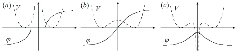
Figure 1: The gravitational kink profile with centripetal deformation (solid line) (a), without deformation (b) and with centripetal deformation (c), together with the corresponding potentials (dashed line).

The solutions corresponding to a negative signature of the extra Kaluza-Klein coordinate $x^{d}$, are once again obtained by changing the sign of the higher dimensional metric. As it has to be expected, in the latter (former) case, spacetime achieves $\textrm{dS}_{3}$ ($\textrm{AdS}_{3}$) at infinity. We find it natural to refer to this classes of solutions as c-kink/anti-c-kink spacetimes and denote them by

$$cK^{3}_{s}(k,l)\hskip 14.22636pt\mbox{and}\hskip 14.22636pt\textrm{A}cK^{3}_{s}(k,l),$$ (72)

with $s=1,2$, where we give in brackets the parameters labeling the solution.

Table 1: Solutions of Grumiller-Jackiw equations.

rank	nullity	solutions
$r=0$	$n=d$	$\mathbb{R}^{d}_{s}(0)$, $\mathbb{R}P^{d}_{s}(k)$, $\mathbb{R}H^{d}_{s}(k)$
$r\geq 2$	$n>1$	$\mathbb{C}P^{\textrm{r}}_{\textrm{s}}\left(\frac{\textrm{F}^{2}}{r}\right)\times\mathbb{R}H^{n}_{s}\left(-\frac{\textrm{F}^{2}}{4r}\right)$, $\mathbb{B}P^{\textrm{r}}\left(\frac{\textrm{F}^{2}}{r}\right)\times\mathbb{R}H^{n}_{s}\left(-\frac{\textrm{F}^{2}}{r}\right)$,
		$\mathbb{C}H^{\textrm{r}}_{\textrm{s}}\left(\frac{\textrm{F}^{2}}{r}\right)\times\mathbb{R}P^{n}_{s}\left(\frac{-\textrm{F}^{2}}{4r}\right)$, $\mathbb{B}H^{\textrm{r}}\left(\frac{\textrm{F}^{2}}{r}\right)\times\mathbb{R}P^{n}_{s}\left(-\frac{\textrm{F}^{2}}{4r}\right)$
$r=2$	$n>1$	$\textrm{A}K^{2}_{1}(k)\times_{4k\tanh^{2}\sqrt{\frac{k}{2}}\xi^{1}}\mathbb{R}P^{n}_{s}\left(2k^{2}\right)$
		$\textrm{A}K^{2}_{1}(k)\times_{-4k\tanh^{2}\sqrt{\frac{k}{2}}\xi^{1}}\mathbb{R}H^{n}_{s}\left(-2k^{2}\right)$
		$K^{2}_{1}(k)\times_{4k\tanh^{2}\sqrt{\frac{k}{2}}\xi^{1}}\mathbb{R}H^{n}_{s}\left(-2k^{2}\right)$
		$K^{2}_{1}(k)\times_{-4k\tanh^{2}\sqrt{\frac{k}{2}}\xi^{1}}\mathbb{R}P^{n}_{s}\left(2k^{2}\right)$
$r\geq 2$	$n=1$	$\mathbb{C}^{\textrm{r}}_{\textrm{s}}\left(0\right)\times^{\pm\sqrt{\frac{|\textrm{F}^{2}|}{r}}J_{\alpha\beta}}\mathbb{R}$, $\mathbb{A}^{\textrm{r}}\left(0\right)\times^{\pm\sqrt{\frac{|\textrm{F}^{2}|}{r}}J_{\alpha\beta}}\mathbb{R}$,
		$\mathbb{C}P^{\textrm{r}}_{\textrm{s}}\left(\mbox{$\frac{\textrm{F}^{2}}{r}\pm\frac{4rl^{2}}{\textrm{F}^{2}}$}\right)\times^{\pm 2l\sqrt{\frac{r}{|\textrm{F}^{2}|}}J_{\alpha\beta}}\mathbb{R}$,
		$\mathbb{B}P^{\textrm{r}}\left(\mbox{$\frac{\textrm{F}^{2}}{r}\pm\frac{4rl^{2}}{\textrm{F}^{2}}$}\right)\times^{\pm 2l\sqrt{\frac{r}{|\textrm{F}^{2}|}}J_{\alpha\beta}}\mathbb{R}$,
		$\mathbb{C}H^{\textrm{r}}_{\textrm{s}}\left(\mbox{$\frac{\textrm{F}^{2}}{r}\pm\frac{4rl^{2}}{\textrm{F}^{2}}$}\right)\times^{\pm 2l\sqrt{\frac{r}{|\textrm{F}^{2}|}}J_{\alpha\beta}}\mathbb{R}$,
		$\mathbb{B}H^{\textrm{r}}\left(\mbox{$\frac{\textrm{F}^{2}}{r}\pm\frac{4rl^{2}}{\textrm{F}^{2}}$}\right)\times^{\pm 2l\sqrt{\frac{r}{|\textrm{F}^{2}|}}J_{\alpha\beta}}\mathbb{R}$
$r=2$	$n=1$	$\textrm{A}cK^{3}_{s}(k,l)$, $cK^{3}_{s}(k,l)$
$r=2\textrm{d}$	$n=0$	$\mathbb{C}P^{\textrm{d}}_{\textrm{s}}\left(\frac{F^{2}}{d}\right)$, $\mathbb{B}P^{\textrm{d}}\left(\frac{F^{2}}{d}\right)$, $\mathbb{C}H^{\textrm{d}}_{\textrm{s}}\left(\frac{F^{2}}{d}\right)$, $\mathbb{B}H^{\textrm{d}}\left(\frac{F^{2}}{d}\right)$

6 Conclusions

We have shown that the equations describing the vanishing of the Weyl conformal tensor in $d+1$-dimensional Kaluza-Klein theories, resembling equations of motion of some $d$-dimensional Einstein-Maxwell-like theory, admit highly symmetric solutions with maximally compatible metric and electromagnetic structures. Null and maximal rank solutions are respectively real and complex/para-complex space forms. Intermediate rank solutions are direct products of real space forms and complex/para-complex space forms with related sectional and holomorphic/para-holomorphic sectional curvatures. Remarkable exceptions are found for nullity-one and rank-two gauge structures. In the former case, solutions are themselves Kaluza-Klein spaces, with metric of a complex/para-complex space form and gauge field proportional to the corresponding complex/para-complex structure. In the latter, the theory supports two dimensional gravitational kinks, mixing with the remaining dimensions through warped products and Kaluza-Klein like structures. The covariant methods developed in Ref. [9] have proven extremely fruitful in obtaining intermediate rank solutions. A summary of our results is presented in Table 1.

References

- [1] D. Grumiller, R. Jackiw, Kaluza-Klein reduction of conformally flat spaces, Int. J. Mod. Phys. D15 (2006) 2075-2094.
- [2] G. Guralnik, A. Iorio, R. Jackiw, S.-Y. Pi, Dimensionally reduced gravitational Chern-Simons term and its kink, Ann. Phys. 308 (2003) 222-236.
- [3] B. O’Neill, Semi-Riemannian geometry with applications to relativity, Academic Press, 1983.
- [4] K. Yano, Differential Geometry on complex and almost complex spaces, Pergamon, 1965.
- [5] M. Barros, A. Romero, Indefinite Kähler manifolds, Math. Ann. 261 (1982) 55-62.
- [6] V. Cruceanu, P. Fortuny, P. M. Gadea, A survey of paracomplex geometry, Rocky Mountain J. Math. 26, n.1 (1996) 83-115.
- [7] P. M. Gadea, A. Montesinos Amilibia, Spaces of constant para-holomorphic sectional curvature, Pacific J. Math. 136, (1989) 85-101.
- [8] P. M. Gadea, J. Muñoz Masqué, Classification of homogeneous parakaehlerian space forms, Nova J. Alg. Geo. 1, (1992) 111-124.
- [9] P. Maraner, J. K. Pachos, Universal features of dimensional reduction schemes from general covariance breaking, Ann. Phys. 323 (2008) 2044-2072.
- [10] D. Grumiller, W. Kummer, The classical solutions of the dimensionally reduced Chern-Simons theory, Ann. Phys. 308 (2003) 211-221.
- [11] P. Maraner, J. K. Pachos, Centrifugal deformations of the gravitational kink, arXiv:0812.0068.