Bouc-Wen-type models with stiffness degradation: thermodynamic analysis and applications

Abstract

In this paper, a thermodynamic analysis of Bouc-Wen models endowed with both strength and stiffness degradation is provided. It is based on the relationship between the flow rules of these models and those of the endochronic plasticity theory with damage, discussed in a companion paper (Erlicher and Point,, 2007). Using the theoretical framework of that extended endochronic theory, it is shown that an elastic Bouc-Wen model with damage, i.e. without plastic strains, can be formulated. Moreover, a proper definition of the dissipated energy of these Bouc-Wen models with degradation is given and some thermodynamic constraints on the parameters defining the models behavior are emphasized and discussed. In particular, some properties of the energetic linear stiffness degradation rule as well as the so-called pivot rule, well-known in the seismic engineering field, are illustrated and commented upon. An improved energetic stiffness degradation rule and a new stiffness degradation rule are proposed.

,

1 Introduction

Bouc, (1967, 1971) developed an univariate model for structural and ferro-magnetic applications. The Bouc’s formulation was similar to the one proposed by Volterra, (1928) to represent hereditary phenomena. However, the clock-time in the Volterra-Stieltjes integrals was substituted by an internal or intrinsic time. The Bouc model was modified by the contributions of several authors; see, among others, Wen, (1976), Karray and Bouc, (1989) and Casciati, (1989), leading to a more general class of models, hereafter named Bouc-Wen-type (BW) models. A further important modification concerned the introduction of the so-called strength and stiffness degradation effects, by means of suitable degradation functions (Baber and Wen,, 1981). In fact, collapse assessment in earthquake engineering requires hysteretic models that include strength and stiffness deterioration properties (Ibarra et al.,, 2005). Some general assumptions on the form of these functions were provided, e.g. they have to be positive and monotone, but no other limitation was mentioned. The resulting hysteresis models were extensively used in the seismic analysis of structural components, e.g. Reinhorn et al., (1995); Foliente, (1995). Moreover, the simplicity of BW models, due to the absence of an elastic domain, allowed their use in stochastic structural analysis. More recently, the BW models were used in applications of structural control, in particular in the modeling of the behavior of magneto-rheological dampers (Sain et al.,, 1997; Jansen and Dyke,, 2000) or other kinds of damping devices (Ikhouane et al.,, 2005). Moreover, several contributions of the last three decades were concerned with the identification of BW model parameters, for applications in seismic engineering; e.g. Masri et al., (2004).

Starting from a different viewpoint and independently from Bouc, Valanis, (1971) proposed the endochronic (EC) theory of visco-plasticity, which postulates the existence of an intrinsic time governing the rate-independent evolution of stress and strain in materials, whereas the Newtonian time is used to model the viscous behavior. In the case of plasticity without viscous effects, it was proven that flow rules can be formulated by using the mathematical formalism of pseudo-potentials. This was done for the standard EC theory by Erlicher and Point, (2006) and for the EC theory with isotropic damage in the companion paper (Erlicher and Point,, 2007).

A major question concerning the BW models is their thermodynamic admissibility. Several criticisms were moved to these models as their formulation was not based on a proper thermodynamic approach. Recently, this problem was analyzed by Ahmadi et al., (1997) and Capecchi and De Felice, (2001) for models without degradation terms. On the other hand, the typical constitutive laws of EC models are characterized by the absence of an elastic domain and the corresponding hysteresis loops are smooth and open, like in the BW models. For this reason several authors, among others, Casciati, (1989) and Sivaselvan and Reinhorn, (2000), observed that a relationship must exist between EC and BW models. A formal proof that all the Bouc-Wen type models with a strength degradation term admit an equivalent endochronic formulation was provided by Erlicher and Point, (2004). This was sufficient to prove that BW models with strength degradation are thermodynamically admissible, in the sense that they fulfill the second principle.

Nonetheless, a problem remains unsolved, viz. the formal proof of the thermodynamic admissibility of BW models endowed with a stiffness degradation term: this is the subject of the present paper. In this respect, the endochronic theory with damage discussed in Erlicher and Point, (2007) is used: it is proved that for every BW model with strength and stiffness degradation, an equivalent EC model with damage can be defined, i.e. a model exhibiting the same flow rules. Therefore, the BW model is thermodynamically admissible if the corresponding EC model fulfills the second principle. Exploiting the aforementioned equivalence, the following results are derived too: (i) a rigorous thermodynamic definition of the plastic strain and of the dissipated energy for BW models exhibiting strength and stiffness degradation; (ii) a new elasto-damaged BW model; (iii) a bound for the stiffness degradation rate of BW models, proving that the traditional semi-empirical stiffness degradation laws, like the energetic linear rule or the so-called pivot rule, may lead to some pathological thermodynamic behavior (these situations are illustrated by several numerical examples); and (iv) an improved energetic stiffness degradation rule and a new stiffness degradation rule.

After the introduction in the first Section, the existing BW models are reviewed in the first three parts of the second Section, while a new class of stress-strain BW models with stiffness degradation is defined in the fourth part. The equivalence between the flow rules of BW models with both degradations and the EC theory with damage is discussed in the third Section. In the fourth Section, single degree-of-freedom (1-DoF) and two-degrees-of-freedom (2-DoF) BW structural models are analyzed in detail, using the theoretical tools previously developed. This analysis is supplemented by some numerical examples and by an application to partial-strength beam-to-column steel joints.

2 Bouc-Wen-type models

A classification of Bouc-Wen-type models is suggested in Figure 1. The main distinction concerns non-degrading models (ND-BW models) and degrading ones. Moreover, among degrading models, the further differentiation between D-BW models having only strength degradation and models characterized by strength and stiffness degradation or by stiffness degradation only (DD-BW models) is pointed out. Then, the models formulated for describing the material behavior by stress-strain laws and the structural behavior by generalized force-displacement laws are distinguished. Note that the box corresponding to stress-strain DD-BW models represents a new class of models, defined by equation (20). In this paper, the equivalence between EC models with isotropic damage (DD-EC), as defined in Erlicher and Point, (2007), and the stress-strain DD-BW models is proven and then used to provide a thermodynamically well-posed formulation for the DD-BW models.

The stress-strain models described in this paper are presented only for a plastically incompressible behavior, since it is the most important case in the literature concerning stress-strain BW models. The treatment of the more general case, with a non-zero hydrostatic plastic flow, is conceptually similar, but requires a more complex formalism not needed here.

2.1 ND-BW models for structures

Among the different models of hysteresis proposed by Bouc, (1971), the simplest one can be formulated by a Stieltjes integral as follows:

$$\left\{\begin{array}[]{l}w\left(t\right)=A_{0}\textrm{ }u\left(t\right)+Z\left(t\right)\\ Z\left(t\right)=\int_{0}^{\xi_{s}\left(t\right)}\mu\left(\xi_{s}\left(t\right)-\xi_{s}^{\prime}\right)\textrm{ }du\left(\xi_{s}^{\prime}\right)\end{array}\right.$$ (1)

where $A_{0}$ is a non-negative constant; $u$ and $w$ are two time-dependent functions, which are considered as input and output functions, respectively. In structural engineering applications the input usually has the meaning of a generalized displacement, while the output $w$ plays the role of a generalized force, defined as the sum of a linear term $A_{0}u(t)$ and a hysteretic term $Z(t)$. The integral in (1)₂ depends on the time-function $\xi_{s}\left(t\right)$, which is named internal time and is assumed to be positive and non-decreasing. The function $\mu$, called the hereditary kernel, takes into account hysteretic phenomena. One of the definitions of $\xi_{s}$ proposed by Bouc is the total variation of $u$:

$$\xi_{s}\left(t\right)=\int_{0}^{t}\left|\frac{du}{dt^{\prime}}\right|dt^{\prime}\textrm{ \ \ or, equivalently, \ \ }\dot{\xi}_{s}=\left|\dot{u}\right|\textrm{, \ with }\xi_{s}\left(0\right)=0\textrm{.}$$ (2)

where the superposed dot indicates time-differentiation. (2) implies the rate-independence of $\xi_{s}$ and as a result, $Z$ and $w$ are in turn rate-independent. Bouc, (1971) defined $\mu$ as a continuous, bounded, positive and non-increasing function on the interval $\xi_{s}\geq 0$, having a bounded integral. In the special case of an exponential kernel

$$\mu\left(\xi_{s}\right)=Ae^{-\beta_{s}\xi_{s}}\textrm{ \ \ \ \ \ \ \ \ \ \ \ \ \ \ \ \ \ \ with \ \ \ }A,\beta_{s}>0$$ (3)

a differential formulation of (1) can be easily deduced. Then, (2) and (3) imply:

$$\left\{\begin{array}[]{l}w=A_{0}\textrm{ }u+Z\\ \dot{Z}=A\textrm{ }\dot{u}-\beta_{s}\textrm{ }Z\textrm{ }\dot{\xi}_{s}\textrm{ \ \ \ \ \ \ \ \ with }\dot{\xi}_{s}=\left|\dot{u}\right|\end{array}\right.$$ (4)

One can observe that for an initial value in the interval $\left(-Z_{u},Z_{u}\right)$, with $Z_{u}=A/\beta_{s}$, the hysteretic force $Z$ remains in the same interval. Bouc, (1967) proposed a more general formulation of (4):

$$\left\{\begin{array}[]{l}w=A_{0}\textrm{ }u+Z\\ \dot{Z}=A\textrm{ }\dot{u}-\beta_{s}\textrm{ }Z\textrm{ }\left|\dot{u}\right|-\gamma_{s}\left|Z\right|\dot{u}\textrm{ \ \ \ \ \ \ \ \ \ \ \ \ \ with \ \ }\gamma_{s}<\beta_{s}\end{array}\right.$$ (5)

while Wen, (1976) suggested a further modification by introducing a positive exponent $n$:

$$\left\{\begin{array}[]{l}w=A_{0}\textrm{ }u+Z\\ \dot{Z}=A\textrm{ }\dot{u}-\left(\beta_{s}\textrm{ }sgn\left(Z\textrm{ }\dot{u}\right)+\gamma_{s}\right)\left|Z\right|^{n}\dot{u}\end{array}\right.$$ (6)

where $sgn(\cdot)$ is the signum function. Wen did not impose any condition on the value of $\gamma_{s}$ and assumed integer values for $n$; however, all real positive values of $n$ are admissible. When $n$ is large enough, force-displacement curves similar to those of an elastic-perfectly-plastic model with the additional linear term $A_{0}u$ are obtained. Provided that $\beta_{s}+\gamma_{s}>0,$ the limit strength value $Z_{u}$ of (6) becomes:

$$Z_{u}=\left(\frac{A}{\beta_{s}+\gamma_{s}}\right)^{\frac{1}{n}}$$ (7)

The parameter $\beta_{s}$ is positive by assumption, while the admissible values for $\gamma_{s}$ can be derived from the condition $\dot{\xi}_{s}\geq 0$ (Erlicher and Point,, 2004). See also Table 1, in this respect.

2.2 Plastically incompressible ND-BW stress-strain models

In order to link the classical plasticity theory and the Bouc-Wen model described in (6), Karray and Bouc, (1989) proposed a tensorial generalization of (6) for isotropic and plastically incompressible materials:

$$\left\{\begin{array}[]{l}tr\left(\mbox{\boldmath$\sigma$}\right)=3E_{1}\textrm{ }tr\left(\mbox{\boldmath$\varepsilon$}\right)+3K\textrm{ }tr\left(\mbox{\boldmath$\varepsilon$}\right)\\ dev\left(\mbox{\boldmath$\sigma$}\right)=2E_{2}\textrm{ }dev\left(\mbox{\boldmath$\varepsilon$}\right)+\mathbf{z}\\ \mathbf{\dot{z}}=2G\textrm{ }dev\left(\mbox{\boldmath$\dot{\varepsilon}$}\right)-\beta\textrm{ }\mathbf{z}\textrm{ }\dot{\xi}\end{array}\right.$$ (8)

with $\beta>0$ and the following special choice for the intrinsic time

$$\dot{\xi}=\left(1+\frac{\gamma}{\beta}\textrm{ }sgn\left(\mathbf{z:}dev\left(\mbox{\boldmath$\dot{\varepsilon}$}\right)\right)\right)\left|\mathbf{z}:dev\left(\mbox{\boldmath$\dot{\varepsilon}$}\right)\right|\left\|\mathbf{z}\right\|^{n-2}$$ (9)

The terms proportional to $E_{1}\geq 0$ and $E_{2}\geq 0$ play the same role as $A_{0}$. $\varepsilon$ and $\sigma$ are the second-order symmetric strain and stress tensors, respectively; $tr$ and $dev$ are the trace and the deviatoric operator, respectively; $\mathbf{z}$ is a traceless tensor defining the hysteretic part of the stress, while $\left\|\mathbf{\cdot}\right\|$ is the standard $L_{2}-norm$ of a symmetric second-order tensor. $K$ and $G$ are the bulk modulus and the shear modulus, respectively. Note that the stress-strain relationship for the traces is linear, according to the assumption of plastic incompressibility. Casciati, (1989) proposed a stochastic analysis of the same model. For this reason, we name it as Karray-Bouc-Casciati (KBC) model. The norm of the tensor $\mathbf{z}\left(t\right)$ is bounded as follows:

$$\left\|\mathbf{z}\right\|=\left\|dev\left(\mbox{\boldmath$\sigma$}\right)-2E_{2}\textrm{ }dev\left(\mbox{\boldmath$\varepsilon$}\right)\right\|<\sigma_{u}=\left(\frac{2G}{\beta+\gamma}\right)^{\frac{1}{n}}$$ (10)

for $t>0$, provided that $\left\|\mathbf{z}\left(0\right)\right\|<\sigma_{u}$. This inequality shows that a limit strength value exists for the KBC model and only regards the deviatoric part of the stress $\sigma$, consistently with the plastic incompressibility requirement. A thermodynamic formulation of this model, based on a suited definition of the Helmholtz free energy and of a pseudo-potential, was proposed in Erlicher and Point, (2006).

2.3 DD-BW models for structures

The BW model (6) was modified by Baber and Wen, (1981), who introduced the positive and increasing functions $\eta_{s}$ and $\nu_{s}$, both having a unit initial value:

$$\left\{\begin{array}[]{l}w=A_{0}\textrm{ }u+Z\\ \dot{Z}=\frac{1}{\eta_{s}}\left[A\textrm{ }\dot{u}-\nu_{s}\left(\beta_{s}\textrm{ }sgn\left(Z\textrm{ }\dot{u}\right)+\gamma_{s}\right)\left|Z\right|^{n}\textrm{ }\dot{u}\right]\end{array}\right.$$ (11)

where $\nu_{s}$ represents a strength degradation effect, while $\eta_{s}$ is associated with a stiffness degradation effect. According to Figure 1, an attentive reader can see that this model belongs to the class of DD-BW models for structures. A degradation function similar to $\eta_{s}$ could also be associated with the post-yielding stiffness $A_{0}$. However, in order to simplify the present analysis, $A_{0}$ is supposed to be constant. In the original formulation of Baber and Wen, (1981), $\eta_{s}$ and $\nu_{s}$ are defined as linearly increasing functions of $e_{s}$, the energy dissipated by the hysteretic model:

$$\nu_{s}=1+c_{\nu,s}\textrm{ }e_{s}\ ,\ \ \ \ \ \eta_{s}=1+c_{\eta,s}\textrm{ }e_{s}$$ (12)

with $c_{\nu,s}\geq 0$ and $c_{\eta,s}\geq 0$. The authors did not provide any definition of $e_{s}$ on a thermodynamic basis. This topic will be discussed later, in the fourth Section. The case of increasing strength, viz. $0<\nu_{s}\leq 1$, is also admissible and it is analogous to isotropic hardening in classical plasticity models. Provided that $\beta_{s}+\gamma_{s}>0$, the maximum strength value, modified by the strength coefficient $r$, becomes

$$Z_{u,red}=\left(\frac{A}{\nu_{s}\textrm{ }\left(\beta_{s}+\gamma_{s}\right)}\right)^{\frac{1}{n}}=\left(\frac{1}{\nu_{s}}\right)^{\frac{1}{n}}Z_{u}=r\ Z_{u}$$ (13)

Several applications of this version of the BW model can be found in the literature; see, among others, Foliente, (1995) and Sivaselvan and Reinhorn, (2000). The latters proposed a formulation of (11) entailing a clear physical meaning of the parameters. Moreover, the following degradation rules were suggested:

$$\left\{\begin{array}[]{l}\nu_{s}=\nu_{s}\left(e_{s},u_{\max}\right)=\left(1-\left(\frac{u_{\max}}{u_{ult}}\right)^{1/\beta_{1}}\right)^{-n}\left(1-\frac{\beta_{2}}{1-\beta_{2}}\frac{e_{s}}{e_{ult}}\right)^{-n}\\ \eta_{s}=\eta_{s}\left(u,w\right)=\frac{A}{R_{k}\left(A+A_{0}\right)-A_{0}}=\frac{A}{\frac{w+\alpha\textrm{ }\tilde{Z}_{u,red}}{\left(A+A_{0}\right)u+\alpha\textrm{ }\tilde{Z}_{u,red}}\left(A+A_{0}\right)-A_{0}}\end{array}\right.$$ (14)

where $u_{\max}=\max_{0\leq\tau\leq t}\left(\left|u\left(\tau\right)\right|\right)$ is the actual value of the maximum displacement modulus; $u_{ult}$ and $e_{ult}$ are defined as the ultimate displacement and the ultimate dissipated energy, corresponding to failure; $\beta_{1}$ and $\beta_{2}$ are positive parameters related to strength degradation; $\alpha$ is a positive parameter related to the stiffness degradation rule (14)₂, called the pivot rule. The sign of $\tilde{Z}_{u,red}=Z_{u,red}$ $sgn\left(u-\frac{w}{\left(A+A_{0}\right)}\right)$ is related to the position of the actual force-displacement point $\left(u,w\right)$ with respect to the line representing the initial elastic behavior $w=\left(A+A_{0}\right)u$.

In summary, the general univariate (also called uniaxial or 1-DoF) BW model reads:

$$\left\{\begin{array}[]{l}w=A_{0}\textrm{ }u+Z\\ \dot{Z}=\frac{1}{\eta_{s}}\left(A\textrm{ }\dot{u}-\beta_{s}\textrm{ }Z\textrm{ }\nu_{s}\dot{\xi}_{s}\right)\end{array}\right.$$ (15)

where $\eta_{s},\nu_{s}$ and $\dot{\xi}_{s}$ can vary from one model to another, as shown in Table 1.

A 2-DoF generalization of (15) was defined by  Park et al., (1986) to represent the behavior of a system constituted of a single mass m subjected to an excitation acting in two orthogonal directions. A simple model associated with this situation is illustrated in Figure 2a. For instance, this model is suited to reproduce the geometrically linear uncoupled behavior of a bi-axially loaded reinforced concrete column (Park et al.,, 1986) or the uncoupled biaxial behavior of a laminated rubber bearing (Abe et al.,, 2004). In the simplest case where the stiffness and the strength are the same in both directions, i.e. isotropic behavior, one has

$$\left\{\begin{array}[]{l}\mathbf{W}=A_{0}\mathbf{U+Z}\\ \mathbf{\dot{Z}=}\frac{1}{\eta_{s}}\left(A\mathbf{\dot{U}}-\beta_{s}\mathbf{Z}\textrm{ }\nu_{s}\dot{\xi}_{s}\right)\end{array}\right.$$ (16)

where $\mathbf{W=}\left(w_{x},w_{y}\right)$ is the total force vector, $\mathbf{U=}\left(u_{x},u_{y}\right)$ is the structural displacement and $\mathbf{Z=}\left(Z_{x},Z_{y}\right)$ is the hysteretic force; the parameters $A_{0}$ and $A$ have the dimension of a stiffness; $\eta_{s}$, $\nu_{s}$ are scalars, since the damage and strength evolution are assumed to be equal in both directions. The intrinsic time $\dot{\xi}_{s}=\dot{\xi}_{s}\left(Z_{x},\dot{u}_{x},Z_{y},\dot{u}_{y}\right)$ and the degradation functions $\nu_{s}$, $\eta_{s}$ may be chosen according to one of the definitions given in Table 2.

An equivalent way of writing (16) is

$$\left\{\begin{array}[]{l}w_{x}=A_{0}\textrm{ }u_{x}+Z_{x}\\ w_{y}=A_{0}\textrm{ }u_{y}+Z_{y}\\ \dot{Z}_{x}=\frac{1}{\eta_{s}}\left(A\textrm{ }\dot{u}_{x}-\beta_{s}\nu_{s}Z_{x}\dot{\xi}_{s}\right)\\ \dot{Z}_{y}=\frac{1}{\eta_{s}}\left(A\textrm{ }\dot{u}_{y}-\beta_{s}\nu_{s}Z_{y}\dot{\xi}_{s}\right)\end{array}\right.$$ (17)

A special case of (17) is given by (Park et al.,, 1986)

$$\left\{\begin{array}[]{l}w_{x}=A_{0}\textrm{ }u_{x}+Z_{x}\\ w_{y}=A_{0}\textrm{ }u_{y}+Z_{y}\\ \dot{Z}_{x}=\frac{1}{\eta_{s}}\left(A\textrm{ }\dot{u}_{x}-\nu_{s}\left[\beta_{s}\textrm{ }Z_{x}\left|Z_{x}\dot{u}_{x}\right|+\gamma_{s}\textrm{ }Z_{x}^{2}\dot{u}_{x}+\beta_{s}\textrm{ }Z_{x}\left|Z_{y}\dot{u}_{y}\right|+\gamma_{s}\textrm{ }Z_{x}Z_{y}\dot{u}_{y}\right]\right)\\ \dot{Z}_{y}=\frac{1}{\eta_{s}}\left(A\textrm{ }\dot{u}_{y}-\nu_{s}\left[\beta_{s}\textrm{ }Z_{y}\left|Z_{y}\dot{u}_{y}\right|+\gamma_{s}\textrm{ }Z_{y}^{2}\dot{u}_{y}+\beta_{s}\textrm{ }Z_{y}\left|Z_{x}\dot{u}_{x}\right|+\gamma_{s}\textrm{ }Z_{x}Z_{y}\dot{u}_{x}\right]\right)\end{array}\right.$$ (18)

which corresponds to a particular choice of the intrinsic time $\dot{\xi}_{s}$, as indicated in the second row of Table 2. Park et al., (1986) assumed $\beta_{s}=\gamma_{s}$ with $A_{0}$ and $\gamma_{s}$ having a special coupled evolution, introduced to obtain force-displacement curves confined in a given envelope. However, we shall assume that $A_{0}$ and $\gamma_{s}$ are constant. The strength degradation $\nu_{s}$ was defined as in (12)₁, while the stiffness degradation $\eta_{s}$ was given by:

$$\eta_{s}=\eta_{s}\left(u_{\max,x},u_{\max,y}\right)=\sqrt{\eta_{x}^{2}+\eta_{y}^{2}}=\sqrt{\left(\frac{u_{\max,x}}{u_{yield}}\right)^{2}+\left(\frac{u_{\max,y}}{u_{yield}}\right)^{2}}\geq 1$$ (19)

where $u_{yield}$ is the yielding displacement, $u_{\max,x}$ and $u_{\max,y}$ are the actual maximum values of the displacement in the two directions $x$ and $y$. The stiffness degradation is therefore governed by the ”uniaxial” ductility ratios $\eta_{x}$ and $\eta_{y}$, while $\eta_{s}$ is a ”bi-axial” ductility ratio.

2.4 Plastically incompressible DD-BW stress-strain models

The KBC model (8)-(9) is a stress-strain BW model characterized by the absence of strength and stiffness degradation. In this subsection, a direct generalization of (8) is proposed, leading a DD-BW model:

$$\left\{\begin{array}[]{l}tr\left(\mbox{\boldmath$\sigma$}\right)=3E_{1}\textrm{ }tr\left(\mbox{\boldmath$\varepsilon$}\right)+\frac{1}{\eta}3K\textrm{ }tr\left(\mbox{\boldmath$\varepsilon$}\right)\\ dev\left(\mbox{\boldmath$\sigma$}\right)=2E_{2}\textrm{ }dev\left(\mbox{\boldmath$\varepsilon$}\right)+\mathbf{z}\\ \mathbf{\dot{z}}=\frac{1}{\eta}\left(2G\textrm{ }dev\left(\mbox{\boldmath$\dot{\varepsilon}$}\right)-\beta\textrm{ }\mathbf{z}\textrm{ }\nu\textrm{ }\dot{\xi}\right)\end{array}\right.$$ (20)

The linearity of the hydrostatic stress-strain law is due to the assumption of plastic incompressibility. The thermodynamic admissibility of the DD-BW model defined in (20), i.e. the conditions under which it fulfills the second principle of thermodynamics, is discussed in the two following Sections. Some simple degradation functions may be defined by analogy with the structural energetic linear rules discussed in the previous subsection, viz.

$$\nu=1+c_{\nu}\textrm{ }e\ ,\ \ \ \ \ \eta=1+c_{\eta}\textrm{ }e$$ (21)

where $e$ is the dissipated  energy per unit volume and the coefficients $c_{\nu},$ $c_{\eta}$ are analogous to $c_{\nu,s},$ $c_{\eta,s}$ introduced in (12). The expressions of $\eta,\ \nu$ and $\dot{\xi}$ for different models are collected in Table 3. As already stated for structural models, the case of increasing strength, viz. $0<\nu\leq 1$, is also admissible and it is analogous to isotropic hardening in classical plasticity.

Models with strength degradation lead to stress-strain laws with softening and, if applied in the continuum setting, to strain localization. It is well-known that an objective description of softening materials and the resulting localized failure modes require special attention. Thus, some of the model parameters must be considered not as pure material properties but as discretization-dependent or, alternatively, the underlying theory must be enriched by special terms, like weighted spatial averages or higher-order gradients, acting as localization limiters (Jirásek and Bažant,, 2002, Chap. 21). These aspects are not the main subject of this paper and therefore are not treated here.

3 Equivalence between DD-BW stress-strain models and endochronic models with damage

The endochronic models with isotropic damage (DD-EC) are discussed in a companion paper (Erlicher and Point,, 2007). We are interested here in the analysis of a DD-EC stress-strain law having the same format as the force-displacement rules (15) and (16), which is defined by the following relationships

$$\left\{\begin{array}[]{l}\mbox{\boldmath$\sigma$}=\mathbf{E}:\mbox{\boldmath$\varepsilon$}+\left(1-D\right)\mathbf{C:}\left(\mbox{\boldmath$\varepsilon-\varepsilon$}^{p}\right)\\ tr\left(\mbox{\boldmath$\dot{\varepsilon}$}^{p}\right)=0\textrm{ \ \ \ \ \ \ \ and \ \ \ \ \ \ \ \ \ }\mbox{\boldmath$\dot{\varepsilon}$}^{p}=\frac{1}{1-D}\frac{dev\left(\mathbf{\sigma-E:\varepsilon}\right)}{2G/\beta}\ \frac{\dot{\zeta}}{g}\end{array}\right.$$ (22)

The non-degrading linear term $\mathbf{E}:\mbox{\boldmath$\varepsilon$}$ is analogous to the term $A_{0}u$ characterizing the models (15) and (16). The tensor $\mbox{\boldmath$\varepsilon$}^{p}$ is the plastic strain. The trace of the plastic strain flow is zero because of the plastic incompressibility assumption; $\mathbf{C}=\left(K-\frac{2G}{3}\right)\mathbf{1\otimes 1}+2G\mathbf{I}$ is the standard elasticity fourth-order tensor for isotropic materials; $\mathbf{E}=\left(E_{1}-\frac{2E_{2}}{3}\right)\mathbf{1\otimes 1}+2E_{2}\mathbf{I}$ is a fourth-order tensor defining an additional elastic stiffness; $\mathbf{1}$ is the second-order identity tensor; $\mathbf{I}$ is the fourth order identity tensor and $\mathbf{\otimes}$ represents the tensor product; $D$ is the scalar damage variable, supposed to be non-negative and less than one; $\zeta$ is called the intrinsic time measure and $\dot{\zeta}\geq 0$ has the role of plastic multiplier (Erlicher and Point,, 2007); $g>0$ is sometimes called the hardening-softening function (Bažant,, 1978). (22) is equivalent to

$$\left\{\begin{array}[]{l}tr\left(\mathbf{\mbox{\boldmath$\sigma$}}\right)=3E_{1}\textrm{ }tr\left(\mbox{\boldmath$\varepsilon$}\right)+\left(1-D\right)3K\textrm{ }tr\left(\mbox{\boldmath$\varepsilon$}\right)\\ dev\left(\mbox{\boldmath$\sigma$}\right)=2E_{2}\textrm{ }dev\left(\mbox{\boldmath$\varepsilon$}\right)+\mathbf{z}\\ \mathbf{\dot{z}}=\left(1-D\right)\textrm{ }2G\textrm{ }dev\left(\mbox{\boldmath$\dot{\varepsilon}$}\right)-\beta\textrm{ }\mathbf{z}\textrm{ }\frac{\dot{\zeta}}{g}-\dot{D}\textrm{ }\frac{\mathbf{z}}{1-D}\end{array}\right.$$ (23)

where the time derivative of the hysteretic deviatoric tensor $\mathbf{z}$ is explicitly written. The comparison of (20) and (23), in particular the definition of $\mathbf{\dot{z}}$, shows that the two models, DD-BW and DD-EC, are equivalent if

$$\nu=\frac{1}{g}\ ,\ \ \ \ \eta=\frac{1}{1-D}\ ,\ \ \ \ \dot{\xi}=\frac{\dot{\zeta}}{1-D}+\dot{D}\textrm{ }\frac{g}{\beta\left(1-D\right)^{2}}$$ (24)

with $\nu\left(0\right)=1,$ $D\left(0\right)=0$ and $\xi\left(0\right)=\zeta\left(0\right)=0$. (24) relate the functions $D$, $g$ and $\zeta$ associated with the DD-EC model and the functions $\eta$, $\nu$ and $\xi$ associated with the DD-BW model. Obviously, this equivalence assumes that the evolution of $D$, $g$ and $\zeta$ can be defined in a way that is general enough to represent all possible evolution of the given $\eta$, $\nu$ and $\xi$. To be more precise, if for instance $\eta$ and $\nu$ are proportional to the dissipated energy, which for DD-BW models may increase during unloading phases, then it should be possible to define $g$ and $D$ of the equivalent endochronic model such that they depend on the dissipated energy, with possible non-zero increments also during unloading phases. The proper thermodynamic framework for DD-EC models allowing this general behavior is presented in a companion paper (Erlicher and Point,, 2007). (24)₁ shows that the function $\nu$ defining the strength increment (degradation) for BW models is strictly related to the function $g$ defining the isotropic hardening (softening) for endochronic models. (24)₂ shows a similar equivalence between the stiffness degradation function of DD-BW models and the isotropic damage variable for DD-EC models. The interpretation of (24)₃ is more involved. It states that the intrinsic time flow $\dot{\xi}$ of a DD-BW model can be expressed as the sum of: (i) a contribution related to the plastic multiplier $\dot{\zeta}$ of the equivalent DD-EC model; (ii) a part related to damage flow $\dot{D}$ of the equivalent DD-EC model. Let us set (24)₃ in the alternative form

$$\dot{\zeta}=\frac{\dot{\xi}}{\eta}-\frac{\dot{\eta}}{\beta\eta\nu}$$ (25)

One can see that (25) is the definition of the plastic multiplier $\dot{\zeta}$ of the DD-EC model equivalent to a given DD-BW model, as a function of $\beta,$ $\dot{\xi},$ $\eta$ and $\nu$. Briefly, (25) defines the plastic multiplier of stress-strain DD-BW models. When $\dot{\zeta}=0$, there is no plastic flow, viz. an elastic with damage behavior is retrieved. Moreover, $\dot{\zeta}=0$ if and only if

$$\dot{\eta}=\frac{\dot{D}}{\left(1-D\right)^{2}}=\beta\nu\dot{\xi}$$ (26)

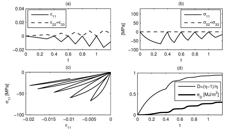
Figure 3: Elasto-damaged BW model, uniaxial stress $\sigma_{11}=\frac{3}{2}[dev(\sigma)]_{11}$. (a) Strain-history $\varepsilon_{11}$ and $\varepsilon_{22}$. (b) $\sigma_{11}$ stress evolution. (c) Stress-strain loops. (d) The damage evolution with the corresponding dissipated energy.

i.e. for DD-BW models, it is possible to obtain zero plastic strains, provided that the special stiffness degradation rule (26) is adopted. Figure 3 shows this behavior, with the parameters $E1=E2=0,$ $2G=24000$ $MPa$, $K=20000$ $MPa$, $\dot{\xi}$ is defined by (9) with $n=1.2$, $\beta=81.2409$ $MPa^{1-n}$, $\gamma/\beta=0.5$ (entailing $\sigma_{u}=100\sqrt{(2/3)}$ $MPa$), $\nu=1+c_{\nu}e$ with $c_{\nu}=0.05$ $m^{3}MJ^{-1}$, $\dot{e}$ is given in (33) underafter and $\dot{\eta}$ is defined by (26).

4 Thermodynamic analysis of DD-BW models

4.1 DD-BW stress-strain models

The thermodynamic analysis of the endochronic model with isotropic damage (DD-EC) presented by Erlicher and Point, (2007) led to the following conditions ensuring thermodynamic admissibility:

$$\begin{array}[]{ll}\dot{D}\geq 0&\textrm{: the damage is non-decreasing}\\ \dot{\zeta}\geq 0&\textrm{: the plastic multiplier is non-negative}\end{array}$$ (27)

These conditions derive from the assumption that the dissipated energy increments owing to plasticity and to damage are separately non-negative. It is well known that this assumption is not needed, since only the total dissipated energy must be non-decreasing. However, this assumption suffices to define models fulfilling the second principle; it is usually adopted (Lemaitre and Chaboche,, 1990) and is also used hereafter. (24)₂ and (27)₁ lead to

$$\dot{\eta}\geq 0\textrm{ : the stiffness degradation function is non-decreasing}$$ (28)

while (24)₃ and (27)_1-2 entail

$$\dot{\xi}\geq 0\textrm{ : the intrinsic time of BW models is non-decreasing}$$ (29)

For DD-BW models, an expression of $\dot{\xi}$ fulfilling (29) is usually given, while $\dot{\zeta}$ is unknown. It follows that the positivity of $\dot{\zeta}$, recall (27)₂, must be ensured by a relevant condition on the stiffness degradation rule, which can easily be derived using (25):

$$\begin{array}[]{l}\dot{\eta}\leq\beta\textrm{ }\nu\ \dot{\xi}\textrm{ : upper bound for the stiffness degradation rate}\end{array}$$ (30)

In summary, two conditions on the stiffness degradation rule are provided: the first one, i.e. (28), is trivial, while the second one, (30), is less obvious. They are obtained using (24) and (25), that relate a DD-BW model, defined by $\dot{\xi}$, $\eta$ and $\nu$, with the equivalent DD-EC model, defined by $\dot{\zeta}$, $D$ and $g$.

The inequality (30) suggests the definition of a new stiffness degradation rule (recall that $\eta\geq 1$):

$$\dot{\eta}=c_{\beta}\left(\frac{1}{\eta}\right)^{m}\textrm{ }\beta\textrm{ }\nu\textrm{ }\dot{\xi}$$ (31)

with $c_{\beta}\in\left[0,1\right]$ and $m\geq 0$. For $m=0$, (31) entails (see also (24)-(25))

$$\dot{\eta}=c_{\beta}\textrm{ }\beta\textrm{ }\nu\textrm{ }\dot{\xi}\textrm{ \ \ }\Longleftrightarrow\textrm{\ \ \ \ }\dot{\zeta}=\left(1-D\right)\textrm{ }\dot{\xi}\left(1-c_{\beta}\right)$$ (32)

i.e. the plastic multiplier is proportional to $\left(1-D\right)$: with the increase of damage, the plastic multiplier decreases. In other words, this rule postulates that plastic strains are larger when the material is slightly damaged and viceversa. When also $c_{\beta}=1$ holds, then $\dot{\zeta}=0$ and an elastic with damage behavior is retrieved, as shown in Figure 3.

Moreover, one can observe that, still using (24)-(25) and recalling that $\mathbf{z=}dev\left(\mbox{\boldmath$\sigma$}-\mathbf{E}:\mbox{\boldmath$\varepsilon$}\right)$, the energies dissipated by plasticity and by damage read:

$$\begin{array}[]{l}\dot{e}=\dot{e}_{p}+\dot{e}_{D}\textrm{ \ \ \ \ \ \ \ with}\\ \dot{e}_{p}=\left(\mathbf{\mbox{\boldmath$\sigma$ }}-\mathbf{E}:\mbox{\boldmath$\varepsilon$}\right):\mbox{\boldmath$\dot{\varepsilon}$}^{p}=\beta\frac{\mathbf{z}:\mathbf{C}^{-1}:\mathbf{z}}{\left(1-D\right)}\left(\left(1-D\right)\nu\textrm{ }\dot{\xi}-\frac{\dot{D}}{\beta\left(1-D\right)}\right)=\frac{\mathbf{z}:\mathbf{z}}{2G}\left(\beta\nu\dot{\xi}-\dot{\eta}\right)\\ \dot{e}_{D}=Y^{d}\dot{D}=\frac{1}{2}\left(\mathbf{\mbox{\boldmath$\sigma$ }}-\mathbf{E}:\mbox{\boldmath$\varepsilon$}\right):\mathbf{C}^{-1}:\left(\mathbf{\mbox{\boldmath$\sigma$ }}-\mathbf{E}:\mbox{\boldmath$\varepsilon$}\right)\frac{\dot{D}}{\left(1-D\right)^{2}}=\frac{1}{2}\left(\frac{\mathbf{z}:\mathbf{z}}{2G}+\frac{\left(tr\left(\sigma-E\varepsilon\right)\right)^{2}}{9K}\right)\dot{\eta}\end{array}$$ (33)

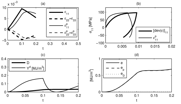
Figure 4: Loading-unloading loop of a BW model, uniaxial stress $\sigma_{11}=\frac{3}{2}[dev(\sigma)]_{11}$. (a) Total and plastic strains. (b) Stress-strain behavior. (c) The evolution of $Y^{d}$ and of the damage. (d) Dissipated energies.

See also the corresponding definitions for DD-EC models in Erlicher and Point, (2007). $Y^{d}$ is the dissipative part of the thermodynamic force dual of the damage variable $D$. Note that the increments of the energy dissipated by plasticity $\dot{e}_{p}$ depend not only on the BW intrinsic time flow $\dot{\xi}$ but also on the flow $\dot{\eta}$ of the stiffness degradation function. Figure 4 shows the evolution of the two terms of the dissipated energy as a function of time. The parameter values are the same of those of Figure 3, except for the ratio $\gamma/\beta=-0.5$ and $\beta=243.7227$ $MPa^{1-n}$; $\nu=1+c_{\nu}e$ with $c_{\nu}=0.05$ $m^{3}MJ^{-1}$; $\eta=1+c_{\eta}e_{p}$ with $c_{\eta}=0.05$ $m^{3}MJ^{-1}$ . Note that there are non-zero plastic strain increments during unloading phases. Moreover, damage increments are always non-zero, also during unloading phases; see also Erlicher and Point, (2007) in this respect.

4.2 DD-BW models for structures

Comparing (20) (that is equivalent to (22) under the conditions previously discussed) with (15) and (16), one can see that structural models have the same format as stress-strain models, provided that stress is replaced by force and strain by displacement, respectively. Analogous substitutions are made for the stiffness tensor, the $\beta,\gamma$ parameters, the degradation functions and the intrinsic time (see the first two columns of Table 4). In the ideal case of a bearing device subjected to bi-directional shear, see Abe et al., (2004) and Figure 2b, the relationships between the stress-strain and force-displacement parameters are given in the third column of Table 4. In general, if a direct derivation of structural models from stress-strain models is not possible, the formal analogy between stress-strain and force-displacement rules must be postulated. Accounting for this analogy and referring to the isotropic 2-DoF model (16), we assume a force-displacement relationship similar to the stress-strain law (22), that reads:

$$\mathbf{W:}=A_{0}\mathbf{U+Z}=A_{0}\mathbf{U+}\frac{1}{\eta_{s}}A\left(\mathbf{U-U}^{p}\right).$$ (34)

The seventh line of Table 4, with the definition of $D_{s}$, has also been used. Moreover, from (16), one has

$$\mathbf{\dot{W}}=A_{0}\mathbf{\dot{U}}+\frac{1}{\eta_{s}}\left[A\mathbf{\dot{U}}-\beta_{s}\mathbf{Z}\textrm{ }\nu_{s}\textrm{ }\dot{\xi}_{s}\right]$$ (35)

Equation (35) and the time-derivative of (34) lead to the definition of the plastic displacement flow

$$\mathbf{\dot{U}}^{p}=\frac{\mathbf{Z}}{A}\left(\beta_{s}\nu_{s}\dot{\xi}_{s}-\dot{\eta}_{s}\right)=\frac{\mathbf{Z}}{A}\beta_{s}\nu_{s}\eta_{s}\left(\frac{\dot{\xi}_{s}}{\eta_{s}}-\frac{\dot{\eta}_{s}}{\beta_{s}\nu_{s}\eta_{s}}\right):=\frac{\mathbf{Z}}{A}\beta_{s}\nu_{s}\eta_{s}\dot{\zeta}_{s}$$

where $\dot{\zeta}_{s}\geq 0$ is a structural plastic multiplier; compare with (25). By analogy with (33) and using Table 4, the rate of energy dissipated by the force-displacement model can be defined as follows:

$$\begin{array}[]{l}\dot{e}_{s}=\dot{e}_{s,p}+\dot{e}_{s,D}\textrm{ \ \ \ \ \ \ \ with}\\ \dot{e}_{s,p}=\mathbf{Z}^{T}\mathbf{\cdot\dot{U}}^{p}=\frac{\mathbf{Z}^{T}\mathbf{\cdot Z}}{A}\textrm{ }\left(\beta_{s}\nu_{s}\dot{\xi}_{s}-\dot{\eta}_{s}\right)\\ \dot{e}_{s,D}:=\frac{\mathbf{Z}^{T}\mathbf{\cdot Z}}{2A}\frac{\dot{D}_{s}}{\left(1-D_{s}\right)^{2}}=\frac{\mathbf{Z}^{T}\mathbf{\cdot Z}}{2A}\textrm{ }\dot{\eta}_{s}\end{array}$$ (36)

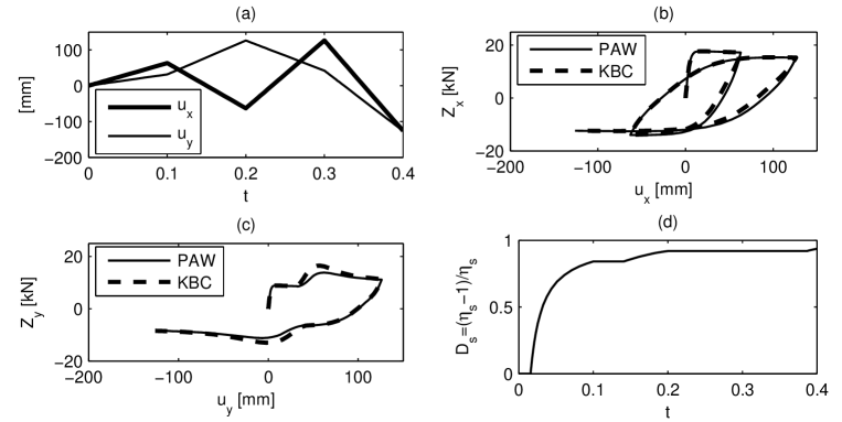
Figure 5: Non-proportional loading of 2-DoF PAW and KBC models. (a) Displacement history for the x- and y-directions. (b) Force-displacement loops $(u_{x},Z_{x})$. (c) Force-displacement loops $(u_{y},Z_{y})$. (d) Damage evolution: the curve is the same for both models; see (19).

All the previous quantities are defined for a 2-DoF BW model; 1-DoF models correspond to deal with scalar quantities instead of vectors. Concerning 2-DoF models, it is interesting to analyze the relationship between the case of an intrinsic time of the Park-Ang-Wen (PAW) type (see the second row of Table 2), versus a 2-DoF model having an intrinsic time of the KBC type with $n=2$ (see the last row of Table 2). It is easy to prove that the intrinsic time flows $\dot{\xi}_{s}$ of the two models become identical in the case of proportional loading. However, they are different in the case of non-proportional loading, leading to different hysteretic loops, as illustrated in Figure 5. The parameters chosen for the numerical simulation are $n=2$, $A_{0}=0$, $A=3.571$ $kN/mm$, $\beta_{s}=0.0119$ $kN^{1-n}mm^{-1}$, $\gamma_{s}=-\beta_{s}/4$. Moreover, the strength degradation is defined by (12)₁ with $c_{\nu,s}=0.0001$ $J^{-1}$, while the stiffness degradation by (19) with $u_{yield}=11.2$ $mm$.

4.2.1 Discussion about the stiffness degradation rule

Conditions (28) and (30) hold at the stress-strain law level. However, taking into account the above-mentioned analysis, the same constraints are postulated at the force-displacement level. As a result, one has

$$\dot{\eta}_{s}\geq 0\ ,\ \ \ \ \dot{\eta}_{s}\leq\beta_{s}\textrm{ }\nu_{s}\textrm{ }\dot{\xi}_{s}$$ (37)

Likewise, also the stiffness degradation rule (31) can be extended to BW models for structures:

$$\dot{\eta}_{s}=c_{\beta}\left(\frac{1}{\eta_{s}}\right)^{m}\textrm{ }\beta_{s}\textrm{ }\nu_{s}\textrm{ }\dot{\xi}_{s}\ \ \ \ \textrm{with}\ \ c_{\beta}\in\left[0,1\right]\ \textrm{and}\ \ m\geq 0$$ (38)

According to the proposed analysis, every stiffness degradation rule defined for structural BW models should be checked with respect to (37). As a result, some bounds for the parameters characterizing these degradation rules may be found. Two examples are considered here: the energetic linear rule, where a possible violation of (37)₂ is highlighted, and the pivot rule, where (37)₁ may not be fulfilled.

The energetic linear rule defined in (12)₂, first adopted in Baber and Wen, (1981), postulates that the stiffness degradation function $\eta_{s}$ depends linearly on the dissipated energy $e_{s}=e_{s,p}+e_{s,D}$, defined in (36):

$$\dot{\eta}_{s}=c_{\eta,s}\ \dot{e}_{s}=c_{\eta,s}\left(\dot{e}_{s,p}+\dot{e}_{s,D}\right)\ \ \rightarrow\dot{\eta}_{s}=\frac{c_{\eta,s}\frac{\mathbf{Z}^{T}\mathbf{\cdot Z}}{A}}{1+c_{\eta,s}\frac{1}{2}\frac{\mathbf{Z}^{T}\mathbf{\cdot Z}}{A}}\beta_{s}\nu_{s}\dot{\xi}_{s}$$ (39)

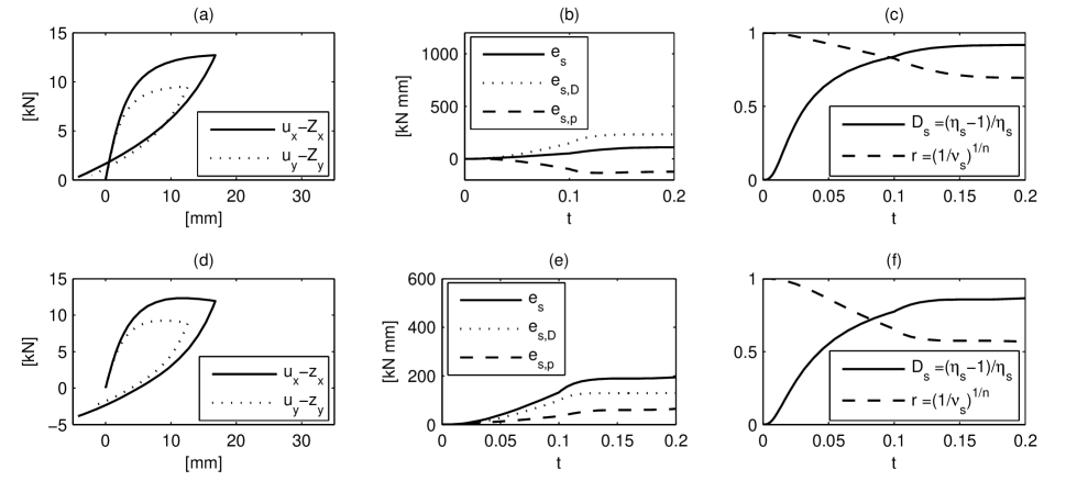
Figure 6: 2-DoF Bouc-Wen model with energetic linear degradation rules. Case of stiffness degradation proportional to $e_{s}$: (a) loading-unloading loop; (b) dissipated energies. Note that $e_{s,p}$ is negative; (c) damage evolution and strength reduction. Case of stiffness degradation proportional to $e_{s,p}$: (d) loading-unloading loop; (e) dissipated energies; (f) damage evolution and strength reduction.

As a result, (37)₂ imposes that the coefficient multiplying $\beta_{s}\nu_{s}\dot{\xi}_{s}$ in (39)₂ be less or equal than one, entailing $c_{\eta,s}\mathbf{\ Z}^{T}\mathbf{\cdot Z}\leq 2A$. This is an upper bound for the parameter $c_{\eta,s}\geq 0$, varying with the actual value of $\mathbf{Z}$. When it is violated, (37)₂ is not satisfied, leading to a negative plastic multiplier, i.e. $\dot{\zeta}_{s}<0$, and to negative increments of the energy dissipated by plasticity, i.e. $\dot{e}_{s,p}<0$. This situation is considered as non-admissible, since it is assumed that the energies dissipated by plasticity and damage must be separately increasing. A numerical simulation where this pathological situation occurs is presented in Figures 6a-c, where a 2-DoF BW model with intrinsic time of KBC type is considered; in detail, $A_{0}=0$, $A=3.5714$ $kN/mm$, $\beta_{s}=0.1308$ $kN^{1-n}mm^{-1}$, $\gamma_{s}=-\beta_{s}/4$ and $n=1.2$. The strength degradation is governed by (12)₁ with $c_{\nu,s}=0.005$ $J^{-1}$, while the stiffness degradation is given by (12)₂ with $c_{\eta,s}=0.1$ $J^{-1}$. Conversely, defining a stiffness degradation rule that depends linearly on the energy dissipated by plasticity

$$\begin{array}[]{l}\eta_{s}=1+c_{\eta,s}e_{s,p}\\ \dot{\eta}_{s}=c_{\eta,s}\textrm{ }\dot{e}_{s,p}=c_{\eta,s}\frac{\mathbf{Z}^{T}\mathbf{\cdot Z}}{A}\left(\beta_{s}\nu_{s}\dot{\xi}_{s}-\dot{\eta}_{s}\right)\textrm{\ \ \ }\rightarrow\textrm{ \ \ }\dot{\eta}_{s}=\frac{c_{\eta,s}\frac{\mathbf{Z}^{T}\mathbf{\cdot Z}}{A}}{1+c_{\eta,s}\frac{\mathbf{Z}^{T}\mathbf{\cdot Z}}{A}}\beta_{s}\nu_{s}\dot{\xi}_{s}\end{array}$$ (40)

the limit condition (37)₂ is always fulfilled. Hence, for a stiffness degradation proportional to the plastic dissipated energy, no limitations are needed on $c_{\eta,s}$. The numerical example illustrated in Figures 6d-f confirms this result. All the model parameters are the same used for the previous case.

The pivot rule (14)₂ is sometimes used for modeling the cyclic behavior of structures; see e.g. Sivaselvan and Reinhorn, (2000) in this respect. Some problems associated with this rule, occurring when it is applied with displacements histories with cycles of decreasing amplitude, were pointed out by Wang and Foliente, (2001). A BW model is considered here, with $A_{0}=0$, $A=50$, $\gamma_{s}=\beta_{s}=0.0189$, $n=1.2$ (entailing $Z_{u}=400$) and $\nu_{s}=1+c_{\nu,s}e_{s}$ with $c_{\nu,s}=1e-6$. The parameter $\alpha$ of the pivot rule is equal to $5$. In this example, the same difficulties mentioned by Wang and Foliente, (2001) appear, viz. the stiffness increases when the cycle amplitude decreases: see Figure 7c. Moreover, a deeper problem is also highlighted: even if the energy dissipated by plasticity and the total dissipated energy are non-decreasing, and the second principle is fulfilled, see Figure 7d, this rule may entail negative damage increments, both during increasing and decreasing amplitude loops. As a result, $\dot{D}_{s}<0\Longleftrightarrow\dot{\eta}_{s}<0$ with a violation of (37)₁, as shown in Figures 7e,f.

Let us now compare the pivot rule to the stiffness degradation rule (38). Figure 7b shows that it is possible to choose the parameters for both rules in such a way to have almost identical force-displacement loops during an initial phase characterized by increasing displacement amplitude cycles. In the specific case considered in the Figure, the new stiffness degradation rule (38) is characterized by $c_{\beta}=0.06$ and $m=1.3$. The damage evolution during this phase for both degradation laws is depicted in Figure 7e: the new degradation rule entails a monotonic increase of damage, consistent with the assumption that dissipated energies by plasticity and damage separately increase; while the pivot rule is characterized by phases with alternate increase and decrease of damage. Then, decreasing amplitude loops are considered for both models and they provide very different behaviors, as illustrated in Figure 7f: the rule (38) still entails an increase of damage, while the pivot rule induces an averaged decrease of damage, corresponding to an averaged increase of stiffness. A similar comparison can be made between the pivot rule and (40). Figure 8 shows the numerical results with $c_{\eta,s}=8.4e-6.$ The same remarks made for Figure 7 hold: Figure 8d shows the evolution of the total dissipated energy for the case of the pivot rule (thin line), the rule (40) (thick line) and the rule (38) considered in the previous example (dotted line). As expected, the pivot rule has a different evolution in the last part of the displacement history, where the stiffness increases instead of decreasing like for the other two rules.

An application application of the BW model (11) with the stiffness degradation (38) and the strength degradation $\nu_{s}=\left(1-\left(\frac{e_{s}}{e_{ult}}\right)^{\frac{1}{\beta_{3}}}\right)^{-n}$, inspired to the rule (14)₁ is shown in Figure 9. In detail, the experimental loops refer to a partial-strength beam-to-column steel joint, studied by Bursi et al., (2002). The assumed parameter values are $A_{0}=1.0$ $kNm/mrad$, $A=21.0$ $kNm/mrad$, $\beta_{s}=0.4888$ $\left(kNm\right)^{1-n}\left(mrad\right)^{-1}$, $\gamma_{s}=0,$ $n=0.8$, $Z_{u}=110$ $kNm$, $e_{ult}=210000$ $Nm$, $\beta_{3}=0.35$, $c_{\beta}=0.02$ and $m=1.8$. For the pivot rule, we assumed $\alpha=4$. An attentive reader can observe that a good agreement between experimental (Figure 9b) and numerical (Figure 9c,d) hysteretic loops is obtained. In addition, the evolution of damage predicted by the model with the rule (38) and with the pivot rule is illustrated in Figure 9e. Again, the drawback of the pivot rule is evident. In summary, one can state that (38) and (40) may be used as a valid alternative to the pivot rule to predict accurate loops; furthermore, they represent a significant improvement in terms of thermodynamic admissibility.

5 Conclusions

An exhaustive classification of Bouc-Wen-type models was provided in this paper. The models endowed with both strength and stiffness degradation were compared with an extended endochronic theory with isotropic damage. The thermodynamic formulation of this extended endochronic theory was discussed in a companion paper (Erlicher and Point,, 2007), using pseudo-potentials depending on state variables and on parameters related to the past history of the material. Using this theoretical framework, a rigorous thermodynamic definition of the energy dissipated by plasticity and damage was provided for Bouc-Wen models having both strength and stiffness degradation, as well as the definition of an elastic with damage Bouc-Wen model. Moreover, an important constraint on the stiffness degradation rules for Bouc-Wen models was highlighted and its consequences on the energetic linear rule were investigated. The non-monotonic damage evolution characterizing the pivot rule was illustrated. Finally, an improved formulation of the energetic linear rule and a new stiffness degradation rule were proposed; their effectiveness with respect to the pivot rule was proved by numerical examples and an application to beam-to-column steel joints.

6 Appendix: Notations

The following symbols are used in this paper:

$A_{0}=$ additional stiffness for structural BW models

$A=$ initial stiffness for structural BW models

$\mathbf{C}=$ fourth-order elasticity tensor

$D=$ internal variable associated with isotropic damage

$\mathbf{E}=$ additional fourth-order elasticity tensor

$E_{1}=$ bulk modulus of the additional elastic behavior

$E_{2}=$ shear modulus of the additional elastic behavior

$K=$ bulk modulus

$G=$ shear modulus

$\mathbf{I}=$ fourth-order identity tensor

$Y^{d}=$ dissipative part of the thermodynamic force dual of the damage variable

$\mathbf{1}=$ second-order identity tensor

$e=$ total dissipated energy per unit volume

$e_{s}=$ total structural dissipated energy

$e_{p}=$ energy per unit volume dissipated by plasticity

$e_{s,p}=$ structural energy dissipated by plasticity

$e_{D}=$ energy per unit volume dissipated by damage

$e_{s,D}=$ structural energy dissipated by damage

$g=$ hardening-softening function for EC models

$u=$ total displacement for 1-DoF BW models

$\mathbf{U}=$ total displacement vector for 2-DoF BW models

$w=$ total force for 1-DoF BW models

$\mathbf{W}=$ total force vector for 2-DoF BW models

$Z=$ hysteretic force for 1-DoF BW models

$\mathbf{z}=$ hysteretic part of the stress tensor

$\mathbf{Z}=$ hysteretic force vector for 2-D0F BW models

$\alpha=$ coefficient associated with the pivot degradation rule

$\beta=$ coefficient characterizing the flow rules of BW or EC stress-strain models

$\beta_{s}=$ coefficient characterizing the flow rules of structural BW models

$\gamma=$ additional coefficient defining the intrinsic time of BW or EC stress-strain models

$\gamma_{s}=$ additional coefficient defining the intrinsic time of structural BW models

$\mbox{\boldmath$\varepsilon$}=$ total small strain tensor

$\mbox{\boldmath$\varepsilon$}^{p}=$ plastic strain tensor

$\mu=$ hereditary kernel

$\nu=$ strength degradation function for BW stress-strain models

$\nu_{s}=$ strength degradation function for BW structural models

$\eta=$ stiffness degradation function for BW stress-strain models

$\eta_{s}=$ stiffness degradation function for BW structural models

$\mbox{\boldmath$\sigma$}=$ Cauchy stress tensor

$\vartheta=$ intrinsic time scale for EC models

$\xi=$ intrinsic time for BW stress-strain models

$\xi_{s}=$ intrinsic time for 1-DoF and 2-DoF BW models

$\zeta=$ intrinsic time measure for EC models; plastic multiplier for stress-strain BW models

$\zeta_{s}=$ structural plastic multiplier for 1-DoF and 2-DoF BW models

	Eq.	$\begin{array}[]{l}\nu_{s},\ \eta_{s}\end{array}$	$\dot{\xi}_{s}$
(Bouc,, 1967) (Bouc,, 1971)	(15)	$1$ ,  $1$	$\left|\dot{u}\right|$
(Bouc,, 1967) (Bouc,, 1971)	(15)	$1$  ,  $1$	$\left(1+\frac{\gamma_{s}}{\beta_{s}}\textrm{ }sgn\left(Z\textrm{ {\ }}\dot{u}\right)\right)\left|\dot{u}\right|$
(Wen,, 1976)	(15)	$1$  ,  $1$	$\left(1+\frac{\gamma_{s}}{\beta_{s}}\textrm{ }sgn\left(Z\textrm{{\ }}\dot{u}\right)\right)\left|\dot{u}\right|\left|Z\right|^{n-1}$ ,  $n>0$
$\begin{array}[]{l}\textrm{\cite[citep]{(\@@bibref{AuthorsPhrase1Year}{Baber81}{\@@citephrase{, }}{})} and}\vspace{-12pt}\\ \lx@intercol\hfil\textrm{\cite[citep]{(\@@bibref{AuthorsPhrase1Year}{Sivaselvan2000}{\@@citephrase{, }}{})}}\hfil\lx@intercol\end{array}$	(15)	$\begin{array}[]{l}\textrm{Eq. }(\ref{rules})\vspace{-12pt}\\ \lx@intercol\hfil\textrm{Eq. }(\ref{rulesSiva})\hfil\lx@intercol\end{array}$	$\left(1+\frac{\gamma_{s}}{\beta_{s}}\textrm{ }sgn\left(Z\textrm{{\ }}\dot{u}\right)\right)\left|\dot{u}\right|\left|Z\right|^{n-1}$,  $n>0$
This paper	(15)	$\begin{array}[]{l}\textrm{Eq. }(\ref{rules})_{1},(\ref{stiffNew1})\vspace{-12pt}\\ \lx@intercol\hfil\textrm{Eq. }(\ref{rulesSiva})_{1},(\ref{stiffNew1})\hfil\lx@intercol\\ \lx@intercol\hfil\textrm{Eq. }(\ref{rules})_{1},(\ref{StiffEnPlast})\hfil\lx@intercol\end{array}$	$\left(1+\frac{\gamma_{s}}{\beta_{s}}\textrm{ }sgn\left(Z\textrm{{\ }}\dot{u}\right)\right)\left|\dot{u}\right|\left|Z\right|^{n-1}$,  $n>0$

Table 1: Summary of the 1-DoF BW models for structures. $\dot{\xi}_{s}\geq 0$, provided that $\left|\gamma_{s}\right|\leq\beta_{s}$. For a thermodynamically admissible model, the stiffness degradation rule fulfills the condition $\dot{\eta}_{s}\leq\beta_{s}\nu_{s}\dot{\xi}_{s}$ (see equation (37)₂).

	Eq.	$\begin{array}[]{l}\nu_{s},\ \eta_{s}\end{array}$	$\dot{\xi}_{s}$
(Park et al.,, 1986)	(16)	Eq. (12)1, (19)	$\left|Z_{x}\textrm{ }\dot{u}_{x}\right|+\left|Z_{y}\textrm{ }\dot{u}_{y}\right|+\frac{\gamma_{s}}{\beta_{s}}\left(Z_{x}\textrm{ }\dot{u}_{x}+Z_{y}\textrm{ }\dot{u}_{y}\right)$
This paper	(16)	$\begin{array}[]{l}\textrm{Eq. }(\ref{rules})\vspace{-12pt}\\ \textrm{Eq. }(\ref{rules})_{1},(\ref{stiffNew1})\end{array}$	$\left|Z_{x}\textrm{ }\dot{u}_{x}\right|+\left|Z_{y}\textrm{ }\dot{u}_{y}\right|+\frac{\gamma_{s}}{\beta_{s}}\left(Z_{x}\textrm{ }\dot{u}_{x}+Z_{y}\textrm{ }\dot{u}_{y}\right)$
This paper	(16)	$\begin{array}[]{l}\textrm{Eq. }(\ref{rules})\vspace{-12pt}\\ \textrm{Eq. }(\ref{rules})_{1},(\ref{stiffNew1})\vspace{-12pt}\\ \textrm{Eq. }(\ref{rules})_{1},(\ref{rulesPAW})\vspace{-12pt}\\ \textrm{Eq. }(\ref{rules})_{1},(\ref{StiffEnPlast})\end{array}$	$\left(1+\frac{\gamma_{s}}{\beta_{s}}\textrm{ }sgn\left(\mathbf{Z}^{T}\cdot\dot{\mathbf{u}}\right)\right)\left|\mathbf{Z}^{T}\cdot\mathbf{\dot{u}}\right|\left\|\mathbf{Z}\right\|^{n-2}$,  $n>0$

Table 2: Summary of the 2-DoF BW models for structures. Both the conditions on the parameter $\gamma_{s}$ and on the stiffness degradation rule recalled in the caption of Table 1 hold for 2-DoF models too. The last definition of $\dot{\xi}_{s}$ is named here of the KBC-type.

	Eq.	$\nu,$ $\eta$	$\dot{\xi}$
(Valanis,, 1971)	(20)	$1$  ,  $1$	$\left\|dev\left(\mbox{\boldmath$\dot{\varepsilon}$}\right)\right\|$
$\begin{array}[]{l}\textrm{\cite[citep]{(\@@bibref{AuthorsPhrase1Year}{Karray89}{\@@citephrase{, }}{})}}\vspace{-12pt}\\ \textrm{and \cite[citep]{(\@@bibref{AuthorsPhrase1Year}{Casciati89}{\@@citephrase{, }}{})}}\end{array}$	(20)	$1$  ,  $1$	$\left(1+\frac{\gamma}{\beta}\textrm{ }sgn\left(\mathbf{z:}dev\left(\mbox{\boldmath$\dot{\varepsilon}$}\right)\right)\right)\left|\mathbf{z}:dev\left(\mbox{\boldmath$\dot{\varepsilon}$}\right)\right|\left\|\mathbf{z}\right\|^{n-2}$, $n>0$
(Erlicher and Point,, 2004)	(20)	$\textrm{Eq. }(\ref{rulesTens})$	$\left(1+\frac{\gamma}{\beta}\textrm{ }sgn\left(\mathbf{z:}dev\left(\mbox{\boldmath$\dot{\varepsilon}$}\right)\right)\right)\left|\mathbf{z}:dev\left(\mbox{\boldmath$\dot{\varepsilon}$}\right)\right|\left\|\mathbf{z}\right\|^{n-2}$, $n>0$
This paper	(20)	$\textrm{Eqs. }(\ref{rulesTens})_{1},(\ref{stiffNew})$	$\left(1+\frac{\gamma}{\beta}\textrm{ }sgn\left(\mathbf{z:}dev\left(\mbox{\boldmath$\dot{\varepsilon}$}\right)\right)\right)\left|\mathbf{z}:dev\left(\mbox{\boldmath$\dot{\varepsilon}$}\right)\right|\left\|\mathbf{z}\right\|^{n-2}$, $n>0$

Table 3: Summary of the BW stress-strain models. Observe that the first BW model coincides with the basic endochronic model proposed by Valanis, (1971). $\dot{\xi}\geq 0$, provided that $\left|\gamma\right|\leq\beta$. For a thermodynamically admissible model, the stiffness degradation rule fulfills the condition $\dot{\eta}\leq\beta\nu\dot{\xi}$ (see equation (30)).

Stress-strain law (20)	Force-displ. laws (15)-(16)	Bearing shear device
$\sigma$ $[Pa]$	$w_{x},w_{y}$ $[N]$	$w_{x}=\sigma_{xz}\textrm{ }S,$ $Z_{y}=\sigma_{yz}\textrm{ }S$
$\mathbf{z}$ $[Pa]$	$Z_{x},Z_{y}$ $[N]$	$Z_{x}=z_{xz}\textrm{ }S,$ $Z_{y}=z_{yz}\textrm{ }S$
$\varepsilon$	$u_{x},u_{y}[m]$	$u_{x}=2h\varepsilon_{xz},$ $u_{y}=2h\varepsilon_{yz}$
$\mathbf{E}$ $(E_{1},E_{2})$ $[Pa]$	$A_{0}$ $[N/m]$	$A_{0}=E_{2}S/h$
$\mathbf{C}$ $(K,G)$ $[Pa]$	$A$ $[N/m]$	$A=GS/h$
$\eta=\frac{1}{1-D},\ \ \nu$	$\eta_{s}:=\frac{1}{1-D_{s}},\ \ \nu_{s}$	$\eta_{s}:=\eta,\ \ \nu_{s}:=\nu$
$\dot{\xi}\left[Pa^{n-1}s^{-1}\right]$	$\dot{\xi}_{s}\left[N^{n-1}ms^{-1}\right]$	$\dot{\xi}_{s}:=\frac{\beta}{\beta_{s}}\dot{\xi}$
$\beta[Pa^{1-n}]$	$\beta_{s}\ [N^{1-n}m^{-1}]$	$\beta_{s}=\frac{S^{1-n}}{h}\left(\sqrt{2}\right)^{n-2}\beta$
$\gamma[Pa^{1-n}]$	$\gamma_{s}\ [N^{1-n}m^{-1}]$	$\gamma_{s}:=\frac{\gamma}{\beta}\beta_{s}=\frac{S^{1-n}}{h}\left(\sqrt{2}\right)^{n-2}\gamma$
$\dot{\zeta}\left[Pa^{n-1}s^{-1}\right]$	$\dot{\zeta}_{s}\left[N^{n-1}ms^{-1}\right]$	$\dot{\zeta}_{s}:=\frac{\beta}{\beta_{s}}\dot{\zeta}$
$e=e_{p}+e_{D}$	$e_{s}=e_{s,p}+e_{s,D}$	$e_{s,p}=Sh$ $e_{p},$ $e_{s,D}=Sh$ $e_{D}$

Table 4: Stress-strain vs. force-displacement rules. In the ideal case of a bearing device subjected to bi-directional shear, see Figure 2b, stresses and strains are uniform in the device volume. Both $\dot{\xi}_{s}$ and $\dot{\xi}$ are postulated to be of the KBC type. $\dot{\xi}_{s},$ $\eta_{s}$ and $\nu_{s}$ are expressed as functions of global quantities like forces and displacements, while $\dot{\xi},$ $\eta$ and $\nu$ depend on local quantities.

Figure 1: Classification of Bouc-Wen-type models.

Figure 2: (a) Scheme of the system associated with the 2-DoF model (16). m is the system mass. (b) An ideal bearing device subjected to bi-directional shear excitation.

Figure 7: Pivot rule (thin line) vs. the new stiffness degradation rule (38)(thick line). (a) Displacement history. (b) Force-displacement loops for the increasing amplitude phase and (c) for the decreasing amplitude phase. (d) Dissipated energy increments for the pivot rule. (e) Damage evolutions for the increasing amplitude phase and (f) for the decreasing amplitude phase.

Figure 8: Pivot rule (thin line) vs. the stiffness degradation rule (40), based on the dissipated energy by plasticity (thick line). (a) Force-displacement loops for the increasing amplitude phase and (b) for the decreasing amplitude phase. (c) Total dissipated energy by the pivot rule and by the plastic energy rule. The dotted line indicates the total energy dissipated in the case of the stiffness rule (38), shown in Figure 7. (d) Damage evolution.

Figure 9: Application to experimental data. (a) Partial strength beam-to-column steel joint JB1-3A (Bursi et al.,, 2002). (b) Experimental Moment-rotation loops: u=$\varphi_{b}-\varphi_{f}$, Z=M_beam (c) Predicted loops with the rule (38). (d) Predicted loops with the pivot rule (14)₂. (e) Damage evolution predicted by the model endowed with the rule (38) (thick line) and by the model with the pivot rule (14)₂ (thin line).

References

- Abe et al., (2004) Abe, M., Yoshida, J., Fujino, Y. (2004). ”Multiaxial behaviors of laminated rubber bearings and their modeling. II: Modeling.” J. Struct. Engrg., 130(8), 1133-1144.
- Ahmadi et al., (1997) Ahmadi, G., Fan, F.-G., and Noori, M.-N. (1997). ”A thermodynamically consistent model for hysteretic materials.” Iranian J. Sci. Tech., 21(3), 257-278.
- Baber and Wen, (1981) Baber, T.T., and Wen, Y.-K. (1981). ”Random vibrations of hysteretic, degrading systems.” J. Engrg. Mech. Div. ASCE, 107(6), 1069-1087.
- Bažant, (1978) Bažant, Z.P. (1978). ”Endochronic inelasticity and incremental plasticity.” Int. J. Solids Struct., 14, 691-714.
- Bouc, (1967) Bouc, R. (1967). ”Forced vibrations of a mechanical system with hysteresis.” Proc. 4th Conference in Nonlinear oscillations, Prague, Czechoslovakia.
- Bouc, (1971) Bouc, R. (1971). ”Modèle mathématique d’hystérésis.” Acustica, 24, 16-25 (in French).
- Bursi et al., (2002) Bursi, O. S., Ferrario, F., Fontanari, V. (2002) ”Non-linear Analysis of the Low-cycle Fracture Behaviour of Isolated Tee Stub Connections.” Computers & Structures, 80, 2333-2360.
- Capecchi and De Felice, (2001) Capecchi, D., and De Felice, G. (2001). ”Hysteretic systems with internal variables.” J. Engrg. Mech., 127(9), 891-898.
- Casciati, (1989) Casciati, F. (1989). ”Stochastic dynamics of hysteretic media.” Struct. Safety, 6, 259-269.