*

Abstract

An elasto-plasticity model with coupled hardening variables of strain type is presented. In the theoretical framework of generalized associativity, the formulation of this model is based on the introduction of two hardening variables with a coupled evolution. Even if the corresponding hardening rules are linear, the stress-strain hardening evolution is non-linear. The numerical implementation by a standard return mapping algorithm is discussed and some numerical simulations of cyclic behaviour in the univariate case are presented.

1 Introduction

Starting from the analysis of the dislocation phenomenon in metallic materials, Zarka and Casier [1] and Kabhou et al. [2] proposed an elasto-plasticity model (”four-parameter model”) where, in addition to the usual kinematic hardening internal variable, a second strain like internal variable was introduced. It plays a role in a modified definition of the von Mises criterion and its evolution, defined by linear flow rules, is coupled with the one of the kinematic hardening variable. The resulting elasto-plastic model depends only on four parameters. Its non-linear hardening behavior was studied in [4] and a parameter identification method using essentially a cyclic uniaxial test was presented in [5] . In this note, the thermodynamic formulation of the classical elasto-plastic model with linear kinematic and isotropic hardening is first recalled. Then, by using the same theoretical framework, a generalization of the four-parameter model is suggested, relying on the introduction of an additional isotropic hardening variable. Finally, a return mapping implementation of the generalized model is presented and some numerical simulations are briefly discussed.

2 Thermodynamic formulation of a plasticity model with linear kinematic/isotropic hardening

Under the assumption of isothermal infinitesimal transformations and of isotropic material, the hydrostatic and the deviatoric responses can be treated separately (see, among others, [7]). Hence, the free energy density $\Psi$ can be split into its spherical part $\Psi_{h}$ and its deviatoric part $\Psi_{d}$. To obtain linear state equations, $\Psi_{h}$ and $\Psi_{d}$ are assumed quadratic. Moreover, experimental results for metals show that permanent strain is only due to deviatoric slip. Hence, an elastic spherical behaviour is assumed, leading to the following definition :

$$\Psi_{h}=\frac{1}{2}\left(\lambda+\frac{2\mu}{3}\right)tr\left(\mathbf{\varepsilon}\right)^{2}=\frac{1}{2}K\text{ }tr\left(\mathbf{\varepsilon}\right)^{2}$$ (1)

where $\mathbf{\varepsilon}$ is the (small) strain tensor, $\lambda$ and $\mu$ are the Lamé constants and $K$ is the bulk modulus. Under the same assumptions, the deviatoric potential $\Psi_{d}$ must depend only on deviatoric state variables. The plastic flow is associated to the plastic strain $\mathbf{\varepsilon}^{p}$, while the kinematic/isotropic hardening behaviour is introduced by the tensorial internal variable $\mathbf{\alpha}$ and by the scalar variable $p$ :

$$\Psi_{d}=\Psi_{d}\left(\mathbf{\varepsilon}_{d}\mathbf{,\varepsilon}^{p},\mathbf{\alpha},p\right)=\frac{2\mu}{2}\left(\mathbf{\varepsilon}_{d}-\mathbf{\varepsilon}^{p}\right):\left(\mathbf{\varepsilon}_{d}-\mathbf{\varepsilon}^{p}\right)+\frac{B}{2}\text{ }\mathbf{\alpha:\alpha+}\frac{H}{2}p^{2}$$ (2)

where $tr\left(\mathbf{\alpha}\right)=tr\left(\mathbf{\varepsilon}^{p}\right)=0$ and $B,\ H>0$ . The evolution of $p$ will be related to the norm of $\mathbf{\varepsilon}^{p}$.
The state equation concerning the deviatoric stress tensor is easily derived:

$$\mathbf{\sigma}_{d}=\frac{\partial\Psi_{d}}{\partial\mathbf{\varepsilon}_{d}}=2\mu\left(\mathbf{\varepsilon}_{d}-\mathbf{\varepsilon}^{p}\right)$$ (3)

and the thermodynamic forces associated to $\mathbf{\varepsilon}^{p},$ $\mathbf{\alpha}$ and $p$ are defined by :

$$\left\{\begin{array}[]{l}\mathbf{\sigma}_{d}=-\frac{\partial\Psi_{d}}{\partial\mathbf{\varepsilon}^{p}}=2\mu\left(\mathbf{\varepsilon}_{d}-\mathbf{\varepsilon}^{p}\right)\\ \mathbf{X}=\frac{\partial\Psi_{d}}{\partial\mathbf{\alpha}}=B\text{ }\mathbf{\alpha}\\ R=\frac{\partial\Psi_{d}}{\partial p}=K\text{ }p\end{array}\right.$$ (4)

One can notice that $tr\left(\mathbf{\varepsilon}\right)=0$. The linearity of the hardening rules (4)_2-3 follows from the quadratic form assumed for the last two terms in (2). The second principle of thermodynamics can be written as follows [7] :

$$\mathbf{\sigma}_{d}:\mathbf{\dot{\varepsilon}}_{d}-\dot{\Psi}_{d}\geq 0$$ (5)

By using (4) in (5), the Clausius Duhem inequality is obtained :

$$\mathbf{\sigma}_{d}:\mathbf{\dot{\varepsilon}}^{p}-\mathbf{X}:\mathbf{\dot{\alpha}}-R\text{ }\dot{p}\geq 0$$ (6)

In order to fulfil this inequality, a classical assumption is to impose that $(\mathbf{\dot{\varepsilon}}^{p},\mathbf{\dot{\alpha}},$ $\dot{p})$ belongs to the subdifferential of a positive convex function $\phi_{d}^{\ast}$, equal to zero in zero, called pseudo-potential. In such a case, the evolution of the internal variables is compatible with (6) [3].

The von Mises criterion corresponds to a special choice for the pseudo-potential $\phi_{d}^{\ast}\left(\mathbf{\sigma}_{d},\mathbf{X},R\right)$ which is equal, in this case, to the indicator function $\mathbb{I}_{f\leq 0}$ of the elastic domain, or, to be more specific, of the set of $\left(\mathbf{\sigma}_{d},\mathbf{X},R\right)$ such that the so-called yielding function $f$ is non-positive :

$$f=f\left(\mathbf{\sigma}_{d},\mathbf{X},R\right)=\left\|\mathbf{\sigma}_{d}-\mathbf{X}\right\|-\sqrt{\frac{2}{3}}\sigma_{y}-R\leq 0$$ (7)

where $\left\|\cdot\right\|$ is the standard $L_{2}$-norm. To impose that $(\mathbf{\dot{\varepsilon}}^{p},\mathbf{\dot{\alpha}},$ $\dot{p})$ belongs to the subdifferential of $\mathbb{I}_{f\leq 0}$ is equivalent to write :

$$\left\{\begin{array}[]{l}\mathbf{\dot{\varepsilon}}^{p}=\dot{\lambda}\frac{\partial f}{\partial\mathbf{\sigma}_{d}}=\dot{\lambda}\frac{\mathbf{\sigma}_{d}-\mathbf{X}}{\left\|\mathbf{\sigma}_{d}-\mathbf{X}\right\|}\\ \mathbf{\dot{\alpha}}=-\dot{\lambda}\frac{\partial f}{\partial\mathbf{X}}=\dot{\lambda}\frac{\mathbf{\sigma}_{d}-\mathbf{X}}{\left\|\mathbf{\sigma}_{d}-\mathbf{X}\right\|}\\ \dot{p}=-\dot{\lambda}\frac{\partial f}{\partial R}=\dot{\lambda}\end{array}\right.$$ (8)

with the conditions $\dot{\lambda}\geq 0$ ,  $f\leq 0$  and $\dot{\lambda}f=0$ .
Equations (8) are called generalized associativity conditions or associative flow rules. The relations (8) yield in this case $\mathbf{\dot{\alpha}}\ =$ $\mathbf{\dot{\varepsilon}}^{p}$ and$\ \dot{\lambda}=\dot{p}=\left\|\mathbf{\dot{\varepsilon}}^{p}\right\|$.
¿From (8)₂ and (4)₂ one obtains the Prager’s linear kinematic hardening rule and a linear isotropic hardening rule :

$$\mathbf{\dot{X}}=B\text{ }\mathbf{\dot{\varepsilon}}^{p}\text{ \ , \ \ \ \ \ }\dot{R}=H\text{ }\dot{p}$$ (9)

The coefficient $\dot{\lambda}$ is strictly positive only if $f=0.$ In this case, its value can be derived from the so-called consistency condition $\dot{f}=0$, i.e.

$$\frac{\partial f}{\partial\mathbf{\sigma}_{d}}:\mathbf{\dot{\sigma}}_{d}\mathbf{+}\frac{\partial f}{\partial\mathbf{X}}:\mathbf{\dot{X}}+\frac{\partial f}{\partial R}\text{ }\dot{R}\text{ }\mathbf{=}\text{ }0$$

The introduction into the previous equation of the state equation (3), as well as the thermodynamic force definitions (4)_2-3 and the normality (8), yield :

$$\frac{\partial f}{\partial\mathbf{\sigma}_{d}}:\mathbf{\dot{\sigma}}_{d}\mathbf{-}\dot{\lambda}\text{ }B\frac{\partial f}{\partial\mathbf{X}}:\frac{\partial f}{\partial\mathbf{X}}-\dot{\lambda}\text{ }H\frac{\partial f}{\partial R}\frac{\partial f}{\partial R}\mathbf{=}0$$ (10)

Moreover, in a strain driven approach, Eq. (10) has to be rewritten still using the state equation (3). As a result, by collecting $\dot{\lambda}$, one obtains

$$\dot{\lambda}=\mathcal{H}\left(f\right)\frac{2\mu\left\langle\frac{\partial f}{\partial\mathbf{\sigma}_{d}}:\mathbf{\dot{\varepsilon}}_{d}\right\rangle}{2\mu\frac{\partial f}{\partial\mathbf{\sigma}_{d}}\text{:}\frac{\partial f}{\partial\mathbf{\sigma}_{d}}+B\frac{\partial f}{\partial\mathbf{X}}\text{:}\frac{\partial f}{\partial\mathbf{X}}+H\frac{\partial f}{\partial R}\frac{\partial f}{\partial R}}=\text{ }\frac{\mathcal{H}\left(f\right)}{1+\frac{B+K}{2\mu}}\frac{\left\langle\left(\mathbf{\sigma}_{d}-\mathbf{X}\right):\mathbf{\dot{\varepsilon}}_{d}\right\rangle}{\left\|\mathbf{\sigma}_{d}-\mathbf{X}\right\|}\geq 0$$

where $\mathcal{H}\left(f\right)$ is zero when $f<0$ and equal to $1$ for $f=0.$ The symbol $\langle.\rangle$ represents the MacCauley brackets.

3 A generalization of the four-parameter model

The linear hardening model discussed previously is used here to suggest a generalization of the 4-parameter model cited in the introduction. The tensor $\mathbf{\alpha}$ into Eq. (2) is replaced by a couple of tensors $(\mathbf{\alpha}_{1},\mathbf{\alpha}_{2})$. As a result, the scalar constant $B$ becomes a $2\times 2$ symmetric positive definite matrix, denoted by $\mathbf{B=[}b_{ij}\mathbf{]}$. For sake of simplicity, only the thermodynamic potential $\Psi_{d}$ is considered here and it is defined as:

$$\Psi_{d}\left(\mathbf{\varepsilon}_{d}\mathbf{,\varepsilon}^{p},\mathbf{\alpha}_{1},\mathbf{\alpha}_{2},p\right)=\frac{2\mu}{2}\left(\mathbf{\varepsilon}_{d}-\mathbf{\varepsilon}^{p}\right)\text{:}\left(\mathbf{\varepsilon}_{d}-\mathbf{\varepsilon}^{p}\right)+\frac{1}{2}\mathbf{\alpha}^{T}\ \mathbf{B\ \alpha}+\frac{H}{2}p^{2}$$

where $\mu$ and $H$ have the same meaning as before and $\mathbf{\alpha}$ is the column vector defined as $\mathbf{\alpha}=[\mathbf{\alpha}_{1};\mathbf{\alpha}_{2}]$. The state equation becomes :

$$\mathbf{\sigma}_{d}=\frac{\partial\Psi_{d}}{\partial\mathbf{\varepsilon}_{d}}=2\mu\left(\mathbf{\varepsilon}_{d}-\mathbf{\varepsilon}^{p}\right)$$ (11)

and the thermodynamic forces have the following form :

$$\left\{\begin{array}[]{l}\mathbf{\sigma}_{d}=-\frac{\partial\Psi_{d}}{\partial\mathbf{\varepsilon}^{p}}=2\mu\left(\mathbf{\varepsilon}_{d}-\mathbf{\varepsilon}^{p}\right)\\ \mathbf{X}_{1}=\frac{\partial\Psi_{d}}{\partial\mathbf{\alpha}_{1}}=b_{11}\text{ }\mathbf{\alpha}_{1}+b_{12}\text{ }\mathbf{\alpha}_{2}\text{ }\\ \mathbf{X}_{2}=\frac{\partial\Psi_{d}}{\partial\mathbf{\alpha}_{2}}=b_{21}\text{ }r\text{ }\mathbf{\alpha}_{1}+b_{22}\text{ }\mathbf{\alpha}_{2}\\ R=\frac{\partial\Psi_{d}}{\partial p}=H\text{ }p\end{array}\right.\qquad\text{or \ \ \ \ \ \ \ }\left\{\begin{array}[]{l}\mathbf{\sigma}_{d}=2\mu\left(\mathbf{\varepsilon}_{d}-\mathbf{\varepsilon}^{p}\right)\\ \mathbf{X}=\mathbf{B\ \alpha}\\ R=H\text{ }p\end{array}\right.$$ (12)

where $\mathbf{X}=[\mathbf{X}_{1};\mathbf{X}_{2}]$. The Clausius -Duhem inequality becomes in this case :

$$\mathbf{\sigma}_{d}:\mathbf{\dot{\varepsilon}}^{p}-\mathbf{X}_{1}:\mathbf{\dot{\alpha}}_{1}-\mathbf{X}_{2}:\mathbf{\dot{\alpha}}_{2}-R\text{ }\dot{p}\geq 0\qquad\text{or \ \ \ \ \ \ \ }\mathbf{\sigma}_{d}:\mathbf{\dot{\varepsilon}}^{p}-\mathbf{X}^{T}\ \mathbf{\dot{\alpha}}-R\text{ }\dot{p}\geq 0$$

Moreover, the loading function $f$ is defined as follows :

$$f=f\left(\mathbf{\sigma}_{d},\mathbf{X}_{1},\mathbf{X}_{2},R\right)=\sqrt{\left\|\mathbf{\sigma}_{d}-\mathbf{X}_{1}\right\|^{2}+\rho^{2}\left\|\mathbf{X}_{2}\right\|^{2}}-\sqrt{\frac{2}{3}}\sigma_{y}-R\leq 0$$ (13)

with $\rho$ a positive scalar. One can remark that for $\rho=0$ and $H=0$ the standard von Mises criterion is derived while for $\rho=1$ and $H=0$ the 4-parameter model is retrieved. The flow rules are defined by a normality condition :

$$\left(\mathbf{\dot{\varepsilon}}^{p},-\mathbf{\dot{\alpha}}_{1},-\mathbf{\dot{\alpha}}_{2},-\dot{p}\right)\in\partial\phi_{d}^{\ast}=\partial\mathbb{I}_{f\leq 0}$$

Therefore, the proposed model belongs to the framework of generalized associative plasticity [3] . The loading function (13) can be rewritten as
$f=g\left(\mathbf{Y}_{1},\mathbf{Y}_{2}\right)-\sqrt{\frac{2}{3}}\sigma_{y}-R\leq 0$ with $\mathbf{Y}_{1}=\mathbf{\sigma}_{d}-\mathbf{X}_{1}$ and $\mathbf{Y}_{2}=-\mathbf{X}_{2}$ . Hence

$$\left\{\begin{array}[]{l}\mathbf{\dot{\varepsilon}}^{p}=\dot{\lambda}\frac{\partial f}{\partial\mathbf{\sigma}_{d}}=\dot{\lambda}\frac{\mathbf{\sigma}_{d}-\mathbf{X}_{1}}{\sqrt{\left\|\mathbf{\sigma}_{d}-\mathbf{X}_{1}\right\|^{2}+\rho^{2}\left\|\mathbf{X}_{2}\right\|^{2}}}\\ \mathbf{\dot{\alpha}}_{1}=-\dot{\lambda}\frac{\partial f}{\partial\mathbf{X}_{1}}=\dot{\lambda}\frac{\mathbf{\sigma}_{d}-\mathbf{X}_{1}}{\sqrt{\left\|\mathbf{\sigma}_{d}-\mathbf{X}_{1}\right\|^{2}+\rho^{2}\left\|\mathbf{X}_{2}\right\|^{2}}}\\ \mathbf{\dot{\alpha}}_{2}=-\dot{\lambda}\frac{\partial f}{\partial\mathbf{X}_{2}}=-\dot{\lambda}\frac{\rho^{2}\text{ }\mathbf{X}_{2}}{\sqrt{\left\|\mathbf{\sigma}_{d}-\mathbf{X}_{1}\right\|^{2}+\rho^{2}\left\|\mathbf{X}_{2}\right\|^{2}}}\\ \dot{p}=-\dot{\lambda}\frac{\partial f}{\partial R}=\dot{\lambda}\end{array}\right.\text{ \ \ or \ \ }\left\{\begin{array}[]{l}\mathbf{\dot{\varepsilon}}^{p}=\dot{\lambda}\frac{\partial f}{\partial\mathbf{\sigma}_{d}}\\ \mathbf{\dot{\alpha}}=\dot{\lambda}\nabla g\\ \dot{p}=\dot{\lambda}\end{array}\right.$$ (14)

It can be seen from (14) that $\mathbf{\dot{\alpha}}_{1}=\mathbf{\dot{\varepsilon}}^{p}$ and $\dot{p}=\dot{\lambda}=\left\|\mathbf{\dot{\alpha}}\right\|=\sqrt{\left\|\mathbf{\dot{\alpha}}_{1}\right\|^{2}+\left\|\mathbf{\dot{\alpha}}_{2}\right\|^{2}}.$ Moreover, from (14)_1-2 and (12)_2-4 one obtains the kinematic and isotropic hardening rules :

$$\mathbf{\dot{X}}_{1}=b_{11}\mathbf{\dot{\varepsilon}}^{p}+b_{12}\text{ }\mathbf{\dot{\alpha}}_{2}\text{, \ \ \ \ \ }\mathbf{\dot{X}}_{2}=b_{21}\mathbf{\dot{\varepsilon}}^{p}+b_{22}\text{ }\mathbf{\dot{\alpha}}_{2}\text{, \ \ \ \ \ }\dot{R}=H\text{ }\dot{p}$$

In [4] it was proved that $\mathbf{B}$ can be written as :

$$\mathbf{B=}\left[\begin{array}[]{cc}\left(A_{\infty}+r^{2}b\right)&-rb\\ -rb&b\end{array}\right]$$

where the scalars $A_{\infty}$ and  $b$ are strictly positive and have the dimension of stresses. For $r=0,$ there is no coupling and $\mathbf{B}$ is diagonal, so that the dimensionless scalar $r$ can be seen as a coupling factor in the evolutions of $\mathbf{X}_{1}$ and $\mathbf{X}_{2}$ :

$$\mathbf{\dot{X}}_{1}=A_{\infty\ }\mathbf{\dot{\varepsilon}}^{p}+rb\text{ }(r\mathbf{\dot{\varepsilon}}^{p}-\mathbf{\dot{\alpha}}_{2})\text{, \ \ }\mathbf{\dot{X}}_{2}=b(r\mathbf{\dot{\varepsilon}}^{p}-\text{ }\mathbf{\dot{\alpha}}_{2})\text{, \ }\Longrightarrow\text{\ \ }\mathbf{\dot{X}}_{1}+r\mathbf{\dot{X}}_{2}=A_{\infty\ }\mathbf{\dot{\varepsilon}}^{p}$$

In the first two flow rules a recalling term appears, as in the non-linear kinematic hardening model of Frederich and Armstrong [8]. As before, the plastic multiplier can be explicitly computed by the consistency condition :

$$\dot{\lambda}=\mathcal{H}\left(f\right)\frac{\left\langle\frac{\partial f}{\partial\mathbf{\sigma}_{d}}:\mathbf{\dot{\varepsilon}}_{d}\right\rangle}{1+\frac{\nabla g.\mathbf{B}.\nabla g+H}{2\mu}}\geq 0.$$

4 Implementation and some numerical results

In this section, a numerical implementation of the model is proposed. A standard return mapping algorithm is considered (see [6]). The formulation is explicitly described in the univariate case, but the tensorial generalization is straightforward. Let $\Delta t_{n}$ be the amplitude of the time step defined by $t_{n}$ and $t_{n+1}$ and let $\mathbf{\tilde{\alpha}}_{n}=\left[\alpha_{1,n},\alpha_{2,n},p_{n}\right]^{T}$  and $\mathbf{\tilde{X}}_{n}=\left[X_{1,n},X_{2,n},R_{n}\right]^{T}$ be the vectors collecting the internal variables and the corresponding thermodynamic forces. Moreover, let

$$\begin{array}[]{l}\mathbf{D}=\left[\begin{array}[]{cc}\mathbf{B}&\mathbf{0}\\ \mathbf{0}&H\end{array}\right]\end{array}$$

be the global hardening modulus matrix. In a strain driven approach, knowing the value of all the variables at the time $t_{n}$ and the strain increment  $\Delta\varepsilon_{n}$ occurring during the time step $t_{n}\rightarrow t_{n+1}$, the numerical scheme computes the variables value at $t_{n+1}$:

$$\left(\varepsilon_{n},\varepsilon_{n}^{p},\mathbf{\tilde{\alpha}}_{n},\sigma_{n},\mathbf{\tilde{X}}_{n},f_{n}\right)+\Delta\varepsilon_{n}\Longrightarrow\left(\varepsilon_{n+1},\varepsilon_{n+1}^{p},\mathbf{\tilde{\alpha}}_{n+1},\sigma_{n+1},\mathbf{\tilde{X}}_{n+1},f_{n+1}\right)$$

The flow equations (14) define a first order differential system, which can be solved by the implicit Euler method. Therefore, the discrete form of the model evolution rules is (the notation $\partial_{\mathbf{w}}f$ is equivalent to $\partial f/\partial\mathbf{w}$) :

$f_{n+1}:=\sqrt{\left(\sigma_{n+1}\mathbf{-}X_{1,n+1}\right)^{2}+\rho^{2}\left(X_{2,n+1}\right)^{2}}-\left(\sigma_{y}+R_{n+1}\right)\leq 0$

$\sigma_{n+1}=E\left(\varepsilon_{n+1}-\varepsilon_{n+1}^{p}\right)$  ;      $\mathbf{\tilde{X}}_{n+1}=\mathbf{D\tilde{\alpha}}_{n+1}$    with $E=\mu\frac{3\lambda+2\mu}{\lambda+\mu}$

$\varepsilon_{n+1}^{p}-\varepsilon_{n}^{p}=\Delta\gamma_{n+1}$ $\partial_{\sigma}f_{n+1}$ ;           $\mathbf{\tilde{\alpha}}_{n+1}-\mathbf{\tilde{\alpha}}_{n}=-\Delta\gamma_{n+1}$ $\partial_{\mathbf{\tilde{X}}}f_{n+1}$

$\Delta\gamma_{n+1}\geq 0,$     $f_{n+1}\leq 0,$     $\Delta\gamma_{n+1}$ $f_{n+1}=0.$

An elastic predictor-plastic corrector algorithm is used to take into account the Kuhn-Tucker conditions [6] (cf the last row). At every time step, in the first predictor phase it holds $f_{n}<0$ , an elastic behaviour is assumed and a trial value of $f_{n+1}$ , i.e. $f_{n+1}^{(0)}$, is computed. If $f_{n+1}^{(0)}\leq 0$ , then an elastic behaviour occurs, $\Delta\gamma_{n+1}$ has to be zero and no corrector phase is required. On the other hand, if $f_{n+1}^{(0)}>0$ , then plastic strains occur, the elastic prediction has to be corrected and $\Delta\gamma_{n+1}>0$ has to be computed. This is done by a suitable return mapping algorithm, described below :

i)

Initialization

$k=0;$ $\varepsilon_{n+1}^{p\left(0\right)}=\varepsilon_{n}^{p},\mathbf{\tilde{\alpha}}_{n+1}^{\left(0\right)}=\mathbf{\tilde{\alpha}}_{n},\gamma_{n+1}^{\left(0\right)}=0$

ii)

Check yield condition and evaluate residuals

$\begin{array}[]{l}\sigma_{n+1}^{\left(k\right)}:=E\left(\varepsilon_{n+1}-\varepsilon_{n+1}^{p\left(k\right)}\right)\text{ \ ; \ }\mathbf{\tilde{X}}_{n+1}^{\left(k\right)}:=\mathbf{D}\text{ }\mathbf{\tilde{\alpha}}_{n+1}^{\left(k\right)}\text{ \ ; \ }f_{n+1}^{\left(k\right)}:=f\left(\sigma_{n+1}^{\left(k\right)},\mathbf{\tilde{X}}_{n+1}^{\left(k\right)}\right)\\ \mathbf{R}_{n+1}^{\left(k\right)}:=\left[\begin{array}[]{c}-\varepsilon_{n+1}^{p\left(k\right)}+\varepsilon_{n}^{p}\\ \mathbf{\tilde{\alpha}}_{n+1}^{\left(k\right)}-\mathbf{\tilde{\alpha}}_{n}\end{array}\right]+\gamma_{n+1}^{\left(k\right)}\left[\begin{array}[]{c}\partial_{\sigma}f\\ \partial_{\mathbf{\tilde{X}}}f\end{array}\right]_{n+1}^{\left(k\right)}\\ \text{if: }f_{n+1}^{\left(k\right)}<tol_{1}\text{ \ \ \ \& \ \ \ }\left\|\mathbf{R}_{n+1}^{\left(k\right)}\right\|<tol_{2}\text{ \ \ \ then: \ EXIT}\end{array}$

iii)

Elastic moduli and consistent tangent moduli

$\begin{array}[]{l}C_{n+1}^{\left(k\right)}=E\text{ \ \ \ \ \ \ \ \ \ }\mathbf{D}_{n+1}^{\left(k\right)}=\mathbf{D}\\ \left(\mathbf{A}_{n+1}^{\left(k\right)}\right)^{-1}=\left[\begin{array}[]{cc}\left(C_{n+1}^{-1}+\gamma_{n+1}\partial_{\sigma\sigma}^{2}f_{n+1}\right)&\gamma_{n+1}\partial_{\sigma\mathbf{\tilde{X}}}^{2}f_{n+1}\\ \gamma_{n+1}\partial_{\mathbf{\tilde{X}}\sigma}^{2}f_{n+1}&\left(\mathbf{D}_{n+1}^{-1}+\gamma_{n+1}\partial_{\mathbf{\tilde{X}\tilde{X}}}^{2}f_{n+1}\right)\end{array}\right]^{\left(k\right)}\end{array}$

iv)

Increment of the consistency parameter

$\Delta\gamma_{n+1}^{\left(k\right)}=\frac{f_{n+1}^{\left(k\right)}-\left[\begin{array}[]{cc}\partial_{\mathbf{\sigma}}f_{n+1}^{\left(k\right)}&\partial_{\mathbf{\tilde{X}}}f_{n+1}^{\left(k\right)}\end{array}\right]^{T}\mathbf{A}_{n+1}^{\left(k\right)}\mathbf{R}_{n+1}^{\left(k\right)}}{\left[\begin{array}[]{cc}\partial_{\sigma}f_{n+1}^{\left(k\right)}&\partial_{\mathbf{\tilde{X}}}f_{n+1}^{\left(k\right)}\end{array}\right]^{T}\mathbf{A}_{n+1}^{\left(k\right)}\left[\begin{array}[]{cc}\partial_{\sigma}f_{n+1}^{\left(k\right)}&\partial_{\mathbf{\tilde{X}}}f_{n+1}^{\left(k\right)}\end{array}\right]^{T}}$

v)

Increments of plastic strain and internal variables

$\left[\begin{array}[]{c}\Delta\varepsilon_{n+1}^{p\left(k\right)}\\ \Delta\mathbf{\tilde{\alpha}}_{n+1}^{\left(k\right)}\end{array}\right]=\left[\begin{array}[]{cc}C_{n+1}^{-1}&0\\ \mathbf{0}&-\mathbf{D}_{n+1}^{-1}\end{array}\right]^{\left(k\right)}\mathbf{A}_{n+1}^{\left(k\right)}\left(\mathbf{R}_{n+1}^{\left(k\right)}+\Delta\gamma_{n+1}^{\left(k\right)}\left[\begin{array}[]{c}\partial_{\sigma}f_{n+1}^{\left(k\right)}\\ \partial_{\mathbf{\tilde{X}}}f_{n+1}^{\left(k\right)}\end{array}\right]\right)$

vi)

Update state variables and consistency parameter

$\varepsilon_{n+1}^{p\left(k+1\right)}=\varepsilon_{n+1}^{p\left(k\right)}+\Delta\varepsilon_{n+1}^{p\left(k\right)}$  ;   $\mathbf{\tilde{\alpha}}_{n+1}^{\left(k+1\right)}=\mathbf{\tilde{\alpha}}_{n+1}^{\left(k\right)}+\Delta\mathbf{\tilde{\alpha}}_{n+1}^{\left(k\right)}$  $\gamma_{n+1}^{\left(k+1\right)}=\gamma_{n+1}^{\left(k\right)}+\Delta\gamma_{n+1}^{\left(k\right)}\vskip 12.0pt plus 4.0pt minus 4.0pt$

This procedure to determine $\Delta\gamma_{n+1}$ requires the computation, at each iteration, of the gradient and the Hessian matrix of $f$ . Other algorithmic approaches by-pass the need of the Hessian of $f$ , but they are not considered here.

This implementation is used to obtain hysteresis loops in some particular cases. The values of the four parameters $E,$ $\sigma_{y},$ $A_{\infty}$ and $b$ are the same as those used in [5] and correspond to the identified values of an Inconel alloy ($E=205580$ Mpa, $\sigma_{y}=1708,9$ Mpa, $A_{\infty}=35500$ Mpa, $b=380700$ Mpa). The value of the new parameter $\rho$ is $\rho=1$ and the values of $r$ and $H$ are indicated in the caption of each figure. /newline Fig. 1 llustrates the hysteresis loops obtained with an increasing amplitude strain history. The effect of the newly introduced isotropic hardening term is highlighted. Fig. 2 refers to a stress input history, with constant amplitude and non-zero mean. The plastic strain accumulation (ratchetting) and the shakedown phenomenon are modelled by changing only one parameter. The hysteresis loops are qualitatively similar to the ones of the non-linear kinematic hardening model of Armstrong and Frederick [8].

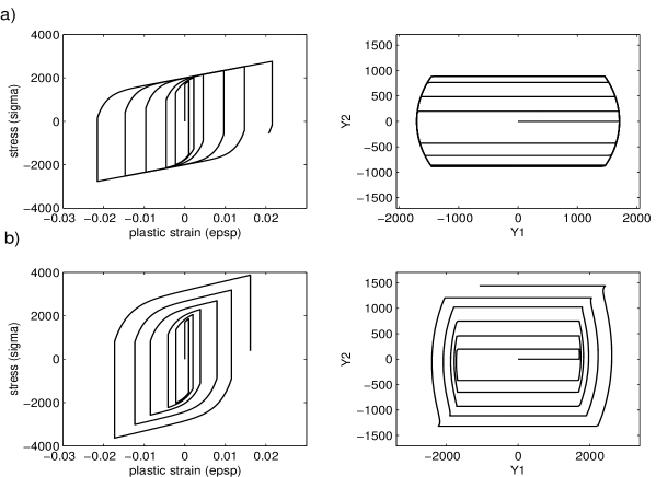
Figure 1: Hysteresis loops for an imposed history with increasing strain amplitude. a) $r=0.608,$ $H=0$ MPa b) $r=0.608,$ $H=6500$ MPa.

5 Conclusions

A model with coupled hardening variables of strain type has been presented. It permits to take into account isotropic hardening and to have an elastic unloading path of varying length depending on the history of the loading. The simplicity of this model, which depends only on six parameters, seems to be very attractive for structural modelling applications with ratchetting effects. To this aim, the proposed return mapping algorithm is a useful numerical tool, which allows numerical simulations to be performed in an effective way.

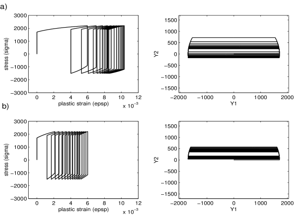
Figure 2: Hysteresis loops for an imposed history with constant stress amplitude and non-zero mean stress. a) $r=0.608,$ $H=0$ MPa; b) $r=0.9,$ $H=0$ MPa.

References

• [1] Zarka J., Casier J. (1979) Elastic plastic response of a structure to cyclic loadings: practical rules. Mechanics Today, 6, Ed. Nemat-Nasser, Pergamon Press
• [2] Khabou M.L., Castex L., Inglebert G. (1985) Eur. J. Mech., A/Solids, 9, 6, 537-549.
• [3] Halphen B., Nguyen Q.S., (1975) Sur les matériaux standards généralisés. J. de Mécanique, 14, 1 , 39-63
• [4] Inglebert G., Vial D., Point N. (1999) Modèle micromécanique à quatre paramètres pour le comportement élastoplastique. Groupe pour l’Avancement de la Mécanique Industrielle, 52, march 1999
• [5] Vial D., Point N. (2000) A Plasticity Model and Hysteresis Cycles. Colloquium Lagrangianum, 6-9 décembre 2000, Taormina, Italy.
• [6] Simo J.C., Hughes T.J.R. (1986), Elastoplasticity and viscoplasticity. Computational aspects.
• [7] J. Lemaitre, J.L. Chaboche (1990), Mechanics of Solid Materials, Cambridge University Press, Cambridge, UK.
• [8] Armstrong P.J., Frederick C.O. (1966), A mathematical representation of the multiaxial Baushinger effect. CEGB Report, RD/B/N731, Berkeley Nuclear Laboratories.