Pseudo-potentials and loading surfaces for an endochronic plasticity theory with isotropic damage

Abstract

The endochronic theory, developed in the early seventies, allows the plastic behavior of materials to be represented by introducing the notion of intrinsic time. With different viewpoints, several authors discussed the relationship between this theory and the classical theory of plasticity. Two major differences are the presence of plastic strains during unloading phases and the absence of an elastic domain. Later, the endochronic plasticity theory was modified in order to introduce the effect of damage. In the present paper, a basic endochronic model with isotropic damage is formulated starting from the postulate of strain equivalence. Unlike the previous similar analyses, in this presentation the formal tools chosen to formulate the model are those of convex analysis, often used in classical plasticity: namely pseudo-potentials, indicator functions, sub-differentials, etc. As a result, the notion of loading surface for an endochronic model of plasticity with damage is investigated and an insightful comparison with classical models is made possible. A damage pseudo-potential definition allowing a very general damage evolution is given.

CE DATABASE SUBJECT HEADINGS: Plasticity, Thermodynamics, Damage, Constitutive models

,

1 Introduction

In the early seventies, Valanis, (1971) proposed the endochronic theory of visco-plasticity, which postulates the existence of an intrinsic time governing the rate-independent evolution of stress and strains in materials, whereas the Newtonian time is exploited to model the viscous behavior; see also (Schapery,, 1968; Bažant and Bath,, 1976). In the case of plasticity without viscous effects, the resulting constitutive laws are characterized by the absence of an elastic domain and the corresponding hysteresis loops are typically smooth and open. The flow rules of these models were not originally formulated in terms of pseudo-potentials, which made the direct comparison of this class of models with classical plasticity theories difficult (Valanis,, 1980). However, it was recently proven by Erlicher and Point, (2006) that endochronic models do admit a representation based on pseudo-potentials and on the normality assumption, provided that pseudo-potentials be endowed with an additional dependence on state variables. This proof, given for the case of plastically incompressible models, showed the strong relationship between the endochronic theory and the generalized plasticity (Phillips and Sierakowski,, 1965; Eisenberg and Phillips,, 1971; Lubliner et al.,, 1993; Auricchio and Taylor,, 1995). It was also shown that the non-linear kinematic hardening model, that is associated, but is not in a generalized sense, admits a representation in terms of a pseudo-potential. Recently, the same authors extended this analysis to other models, like the Mróz model (Point and Erlicher,, 2007) and the non-associated Drucker-Prager model (Erlicher and Point,, 2005); see also Ziegler and Wehrli, (1987), Houlsby and Puzrin, (2000). In summary, this thermodynamically well-posed approach can be used for a very large class of existing classical or non-classical plasticity models. Actually, a similar approach is used in geotechnical engineering, see e.g. Collins and Houlsby, (1997), where pseudo-potentials have an additional dependence on the so-called true stresses, distinguished from the generalized stresses.

The standard endochronic theory was modified by several authors through the introduction of a damage variable. Using the strain equivalence postulate, Xiaode, (1989) proposed an endochronic model with isotropic damage, while Valanis, (1990) discussed an endochronic model with anisotropic damage, in the larger theoretical framework of fracture mechanics. Later, a different approach based on the postulate of energy equivalence was used, among others, by Chow and Chen, (1992) and Wu and Nanakorn, (1998, 1999).

In the aforementioned works, the thermodynamic formulation of flow rules is not based on the notions of pseudo-potentials and loading surfaces, as it is typical for other classical plasticity models with or without damage. Hence, in this paper, a simple endochronic model of plasticity with isotropic damage similar to that discussed by Xiaode, (1989) is presented: no generalization is introduced with respect to the previously cited models, but a new approach is suggested for their description. In detail, the postulate of strain equivalence is adopted; the Helmholtz energy is assumed to have a regular quadratic term and an additional singular term; the tools of the convex analysis such as indicator functions and sub-differentials (Rockafellar,, 1969; Moreau,, 1970; Frémond,, 2002) are used to define the flow rules starting from well-suited pseudo-potentials. This presentation leads to the proper definition of the plasticity loading surface for an endochronic model with damage and is a direct extension of the results concerning the endochronic model without damage already discussed in Erlicher and Point, (2006). Only plastically incompressible models are considered here, since they permit to explain the main ideas, without introducing a too complex formalism. The extension to the general case is possible, but it is omitted for simplicity. The proposed analysis has an intrinsic interest, since it allows an easier comparison between endochronic models with damage and classical plasticity models with damage. Nonetheless, in the authors’ opinion, another important reason justifies the interest towards this class of models: they represent the suitable theoretical basis for the analysis of the thermodynamic admissibility of the Bouc-Wen models with strength and stiffness degradation; see among others (Bouc,, 1971; Wen,, 1976; Baber and Wen,, 1981; Casciati,, 1989; Karray and Bouc,, 1989). This was one of the main motivation at the origin of the present study and the related developments about degrading Bouc-Wen models are presented in a companion paper (Erlicher and Bursi,, 2007).

After the introduction, the endochronic theory is presented in the second section: in the first part, standard endochronic models are described, while the second part concerns the definition of the flow rules of the extended endochronic theory, characterized by an additional scalar variable endowed with damage. The thermodynamic framework, with the definition of the suited pseudo-potentials, is discussed in the following section and is supplemented by numerical examples. Then, a brief discussion about stability and uniqueness is made and the concluding remarks are given, where the topics dealt with in the companion paper (Erlicher and Bursi,, 2007) are pointed out.

2 Endochronic models

2.1 Flow rules of plastically incompressible ND-EC models

The endochronic theory was first formulated by Valanis, (1971), who suggested the use of a positive scalar variable $\vartheta$, called the intrinsic time scale, in the definition of constitutive plasticity models. The evolution laws are described by convolution integrals involving past values of the strain $\varepsilon$ and suitable scalar functions $\mu$ depending on $\vartheta$, called memory kernels. When the memory kernel is exponential, the integral expressions can be rewritten as simple differential equations, the flow rules; in the case of an isotropic endochronic model without hardening or softening, called here ND-EC model (see Figure 1), fulfilling the plastic incompressibility assumption, they read:

$$\left\{\begin{array}[]{l}tr\left(\mbox{\boldmath$\sigma$}\right)=3K\ tr\left(\mbox{\boldmath$\varepsilon$}\right),\text{ \ \ \ \ \ }dev\left(\mbox{\boldmath$\sigma$}\right)=\mathbf{z}\\ \mathbf{\dot{z}}=2G\ dev\left(\mbox{\boldmath$\dot{\varepsilon}$}\right)\mathbf{-}\beta\ \mathbf{z}\dot{\vartheta}\end{array}\right.$$ (1)

where $\beta>0$ (notice that $\beta$ different from zero is needed to have a non elastic behavior); the superposed dot indicates the time derivative; $\varepsilon$ is the small strain tensor; $\sigma$ is the Cauchy stress tensor; $tr$ and $dev$ are the trace and deviatoric operators; $K$ is the bulk modulus while $G$ is the shear modulus. The simplest choice for the intrinsic time scale flow indicated in (1) is $\dot{\vartheta}=\left\|dev\left(\mbox{\boldmath$\dot{\varepsilon}$}\right)\right\|$. It is interesting to note that relationships (1) are equivalent to

$$\left\{\begin{array}[]{l}\mbox{\boldmath$\sigma$ }=\mathbf{C:}\left(\mbox{\boldmath$\varepsilon-\varepsilon$ }^{p}\right)\\ tr\left(\mbox{\boldmath$\dot{\varepsilon}$}^{p}\right)=0\text{ \ \ \ \ \ \ \ and \ \ \ \ \ \ \ \ \ }\mbox{\boldmath$\dot{\varepsilon}$}^{p}=\beta\frac{dev\left(\sigma\right)}{2G}\ \dot{\vartheta}\end{array}\right.$$ (2)

where the trace of the plastic strain flow $\dot{\mbox{\boldmath$\varepsilon$}}^{p}$ is zero, consistently with the assumption of plastic incompressibility. $\mathbf{C}=\left(K-2G/3\right)\mathbf{1\otimes 1}+2G\mathbf{I}$ is the elasticity fourth-order tensor for isotropic materials; $\mathbf{1}$ is the second-order identity tensor; $\mathbf{I}$ is the fourth-order identity tensor and $\mathbf{\otimes}$ represents the tensor product.

2.2 Flow rules of plastically incompressible D-EC and DD-EC models

An endochronic model with isotropic hardening or softening with plastically incompressible flow is defined as follows:

$$\left\{\begin{array}[]{l}tr\left(\mathbf{\mbox{\boldmath$\sigma$ }}\right)=3K\text{ }tr\left(\mbox{\boldmath$\varepsilon$ }\right)\text{ , \ \ \ \ \ \ \ \ \ }dev\left(\mbox{\boldmath$\sigma$ }\right)=\mathbf{z}\\ \mathbf{\dot{z}}=2G\text{ }dev\left(\mbox{\boldmath$\dot{\varepsilon}$}\right)-\beta\text{ }\mathbf{z}\text{ }\dot{\vartheta}\text{ \ \ \ \ }\ \ \ \ \ \text{with }\dot{\vartheta}=\frac{\dot{\zeta}}{g}\end{array}\right.$$ (3)

where $g>0$ is called the hardening-softening function (Bažant,, 1978). As stated by its name, the function $g$ introduces isotropic hardening (or softening), which distinguishes this model (D-EC) from the basic ones presented in the previous section and indicated as ND-EC (see Figure 1). In the classical endochronic formulations, $g$ is a function of $\zeta$, where $\zeta$ is the intrinsic time measure. A standard choice is $\dot{\zeta}=\left\|dev\left(\mbox{\boldmath$\dot{\varepsilon}$}\right)\right\|$ according to Valanis, (1971). Another more general definition, leading to a cyclic behavior similar to that of the Prandtl-Reuss model (Lemaitre and Chaboche,, 1990) when the positive parameter $n$ is large enough, reads

$$\dot{\zeta}=\left(1+\frac{\gamma}{\beta}sgn\left(\mathbf{z}:dev\left(\mbox{\boldmath$\dot{\varepsilon}$}\right)\right)\right)\left|\mathbf{z}:dev\left(\mbox{\boldmath$\dot{\varepsilon}$}\right)\right|\left\|\mathbf{z}\right\|^{n-2}$$ (4)

with $\gamma\in\left[-\beta,\beta\right]$ in order to ensure the non-negativity of $\dot{\zeta}$; $sgn$ is the signum function. An important difference between (4) and the standard definition $\dot{\zeta}=\left\|dev\left(\mbox{\boldmath$\dot{\varepsilon}$}\right)\right\|$ is related to the product $\mathbf{z}:dev\left(\mbox{\boldmath$\dot{\varepsilon}$}\right)$, entailing $\dot{\zeta}=0$ when the deviatoric strain increment is orthogonal to the stress. However, $\dot{\zeta}$ can be different from zero during unloading, i.e. when $\mathbf{z}:dev\left(\mbox{\boldmath$\dot{\varepsilon}$}\right)<0$. Eq. (4) shows that $\gamma$ affects the difference between the loading and unloading values of the intrinsic time increment at a given stress $\mathbf{z}$. In particular, when $\gamma=\beta$ these increments are zero during unloading, while $\gamma$ close to (and greater than) $-\beta$ leads to relatively small increments during loading, while $\dot{\zeta}$ is relatively large during unloading. The influence of $n$ on the endochronic model behavior is discussed in the last Section, with reference to the strain accumulation and the stress relaxation effects. According to (3) and (4) and assuming $\beta+\gamma>0$, the norm of the tensor $\mathbf{z}\left(t\right)$ is bounded as follows:

$$\left\|\mathbf{z}\left(t\right)\right\|=\left\|dev\left(\mbox{\boldmath$\sigma$}\left(t\right)\right)\right\|<\sigma_{u}=\left(\frac{2G}{\beta+\gamma}\right)^{\frac{1}{n}}$$ (5)

for $t>0$, provided that $\left\|\mathbf{z}\left(0\right)\right\|<\sigma_{u}$. This inequality proves that a limit strength value exists and only concerns the deviatoric part of the stress $\sigma$, consistently with the plastic incompressibility requirement. Eq. (5) also shows that this bounding stress depends on the parameters $\beta,$ $\gamma$ and $n$.

The expression (3) is equivalent to

$$\left\{\begin{array}[]{l}\mbox{\boldmath$\sigma$ }=\mathbf{C:}\left(\mbox{\boldmath$\varepsilon-\varepsilon$ }^{p}\right)\\ tr\left(\mbox{\boldmath$\dot{\varepsilon}$}^{p}\right)=0\text{ \ \ \ \ \ \ \ and \ \ \ \ \ \ \ \ \ }\mbox{\boldmath$\dot{\varepsilon}$}^{p}=\frac{dev\left(\mathbf{\sigma}\right)}{2G/\beta}\ \frac{\dot{\zeta}}{g}\end{array}\right.$$ (6)

From the last relationship in (6), it appears that the parameters $\beta,\gamma$ and $n$ introduced in (4) affect the amplitude of the plastic strain flow, while the direction is always that of $dev\left(\mbox{\boldmath$\sigma$}\right)$.

A larger class of endochronic models can be defined by the following relationships

$$\left\{\begin{array}[]{l}\mbox{\boldmath$\sigma$ }=\left(1-D\right)\mathbf{C:}\left(\mbox{\boldmath$\varepsilon-\varepsilon$ }^{p}\right)\\ tr\left(\mbox{\boldmath$\dot{\varepsilon}$}^{p}\right)=0\text{ \ \ \ \ \ \ \ and \ \ \ \ \ \ \ \ \ }\mbox{\boldmath$\dot{\varepsilon}$}^{p}=\frac{1}{1-D}\frac{dev\left(\mathbf{\sigma}\right)}{2G/\beta}\ \frac{\dot{\zeta}}{g}\end{array}\right.$$ (7)

where $D$ is a scalar variable introducing isotropic damage. The plasticity model with damage defined by (7) is named here the extended endochronic model and it belongs to the class of DD-EC models, as indicated in Figure 1. Note that the stress is defined by introducing the factor $\left(1-D\right)$, consistently with the definition of effective stress and the principle of strain equivalence (Lemaitre and Chaboche,, 1990). Moreover, it can be observed that the relationships (7) are equivalent to

$$\left\{\begin{array}[]{l}tr\left(\mathbf{\mbox{\boldmath$\sigma$}}\right)=\left(1-D\right)3K\text{ }tr\left(\mbox{\boldmath$\varepsilon$}\right)\text{ , \ \ \ \ \ \ \ }dev\left(\mbox{\boldmath$\sigma$}\right)=\mathbf{z}\\ \mathbf{\dot{z}}=\left(1-D\right)\text{ }2G\text{ }dev\left(\mbox{\boldmath$\dot{\varepsilon}$}\right)-\beta\text{ }\mathbf{z}\text{ }\dot{\vartheta}-\dot{D}\text{ }\frac{\mathbf{z}}{1-D}\text{ \ \ \ \ }\ \ \ \ \ \text{with }\dot{\vartheta}=\frac{\dot{\zeta}}{g}\end{array}\right.$$ (8)

which can be compared with (3).

A possible choice for $\dot{\zeta}$ is given by

$$\dot{\zeta}=\left(1+\frac{\gamma}{\beta}sgn\left(\mathbf{z}:dev\left(\mbox{\boldmath$\dot{\varepsilon}$}\right)\right)\right)\left|\mathbf{z}:dev\left(\mbox{\boldmath$\dot{\varepsilon}$}\right)\right|\left\|\mathbf{z}\right\|^{n-2}\left(1-D\right)^{1-n}$$ (9)

which represents a direct generalization of (4): the last factor depending on $D$ and $n$ is introduced in order to have an intrinsic time depending on the effective stress instead of the actual one, consistently with the strain equivalence postulate. An elastic with damage model can be defined by assuming $\dot{\zeta}=0$. In the authors’ knowledge, the notions of pseudo-potential and loading surface were never applied to the extended endochronic theory; therefore, these aspects are analyzed in detail in the next section.

3 A thermodynamic framework for the extended endochronic theory

The aim of this section is to define the Helmholtz free energy and the pseudo-potential leading to the flow rules (7) or, equivalently, (8). Under the assumption of isothermal and small transformations, the Helmholtz free energy density is chosen as follows:

$$\Psi=\Psi\left(\mathbf{v}\right)=\psi\left(\mbox{\boldmath$\varepsilon$},\mbox{\boldmath$\varepsilon$}^{p}\mathbf{,}\zeta\mathbf{,}D\right)+\mathbb{I}_{\mathbb{H}}\left(\mbox{\boldmath$\varepsilon$},\mbox{\boldmath$\varepsilon$}^{p}\mathbf{,}\zeta\mathbf{,}D\right)$$ (10)

where $\mathbf{v}=\left(\mbox{\boldmath$\varepsilon$},\mbox{\boldmath$\varepsilon$}^{p}\mathbf{,}\zeta\mathbf{,}D\right)$ is the vector of state variables; $\varepsilon$, $\mbox{\boldmath$\varepsilon$}^{p}$ and $D$ were previously defined; $\zeta$ is a scalar internal variable associated with isotropic hardening. For all the state variables, an initial zero value is assumed. The choice of $\zeta$ to indicate an internal variable might seem misleading, since the symbol $\zeta$ was also used in (3)-(8) to define the intrinsic time measure. However, as it will be seen hereafter, this choice is the proper one, as for endochronic models, $\zeta$ has simultaneously both meanings; $\psi$ is the regular part of the Helmholtz energy; $\mathbb{I}_{\mathbb{H}}$ is the indicator function of the closed set $\mathbb{H}$: by definition, an indicator function is equal to $0$ inside $\mathbb{H}$ and equal to $+\infty$ outside (Rockafellar,, 1969); the set $\mathbb{H}$ indicates the admissibility domain for the state variables $\mathbf{v}$ and should be introduced every time some conditions on state variables are to be imposed: for instance, it is equal to the interval $D\in[0,1]$ in order to impose the admissible values for the damage variable (Frémond,, 2002).

Once $\Psi$ is known, the non-dissipative thermodynamic forces $\mathbf{q}^{nd}=(\mbox{\boldmath$\sigma$}^{nd},\mbox{\boldmath$\tau$}^{nd},R^{nd},Y^{nd})$ are defined as the gradient of $\psi\left(\mbox{\boldmath$\varepsilon$},\mbox{\boldmath$\varepsilon$}^{p}\mathbf{,}\zeta\mathbf{,}D\right)$:

$$\mbox{\boldmath$\sigma$}^{nd}:=\frac{\partial\psi}{\partial\mbox{\boldmath$\varepsilon$}},\text{ \ \ }\mbox{\boldmath$\tau$}^{nd}:=\frac{\partial\psi}{\partial\mbox{\boldmath$\varepsilon$}^{p}},\text{ \ \ }R^{nd}:=\frac{\partial\psi}{\partial\zeta},\text{ \ \ }Y^{nd}:=\frac{\partial\psi}{\partial D}$$ (11)

while the non-dissipative reaction forces $\mathbf{q}^{ndr}=(\mbox{\boldmath$\sigma$}^{ndr},\mbox{\boldmath$\tau$}^{ndr},R^{ndr},Y^{ndr})$ are given by

$$\left(\mbox{\boldmath$\sigma$}^{ndr},\mbox{\boldmath$\tau$}^{ndr},R^{ndr},Y^{ndr}\right)\in\partial\mathbb{I}_{\mathbb{H}}\left(\mbox{\boldmath$\varepsilon$},\mbox{\boldmath$\varepsilon$}^{p}\mathbf{,}\zeta\mathbf{,}D\right)$$ (12)

where $\partial$ is the sub-differential operator (Rockafellar,, 1969). If the constraints imposed by $\mathbb{H}$ are fulfilled, the indicator function $\mathbb{I}_{\mathbb{H}}$ is zero and $\Psi\left(t\right)=\psi\left(t\right)$. This entails the identity of the time-derivatives, viz. $\dot{\Psi}\left(t\right)=\dot{\psi}\left(t\right)+\mathbf{q}^{ndr}\cdot\mathbf{\dot{v}}=\dot{\psi}\left(t\right)$. In other words, one has $\mathbf{q}^{ndr}\cdot\mathbf{\dot{v}=}0$ for every instant $t$ (Frémond,, 2002).

Due to the assumptions of isothermal and small transformations, the expression of the second principle reads:

$$\Phi_{1}\left(t\right)=\mbox{\boldmath$\sigma:\dot{\varepsilon}$}-\dot{\psi}\geq 0$$ (13)

(13) states that the intrinsic (or mechanical) dissipation $\Phi_{1}$ has to be non-negative. Introducing the dissipative thermodynamic forces $\mathbf{q}^{d}=(\mbox{\boldmath$\sigma$}^{d},\mbox{\boldmath$\tau$}^{d},R^{d},Y^{d})$ as

$$\mbox{\boldmath$\sigma$}^{d}:=\mbox{\boldmath$\sigma-\sigma$}^{nd}-\mbox{\boldmath$\sigma$}^{ndr}\text{ ,\ \ \ \ \ }\mbox{\boldmath$\tau$}^{d}:=-\mbox{\boldmath$\tau$}^{nd}-\mbox{\boldmath$\tau$}^{ndr},\text{\ \ \ \ }R^{d}:=-R^{nd}-R^{ndr},\text{\ \ \ \ }Y^{d}:=-Y^{nd}-Y^{ndr}$$ (14)

and substituting (14) in (13), one obtains:

$$\Phi_{1}\left(t\right)=\mbox{\boldmath$\sigma$}^{d}:\mbox{\boldmath$\dot{\varepsilon}$}+\mbox{\boldmath$\tau$}^{d}:\mbox{\boldmath$\dot{\varepsilon}$}^{p}+R^{d}\dot{\zeta}+Y^{d}\text{ }\dot{D}\text{ }\mathbf{\geq}\text{ }0$$ (15)

In order to fulfill (15), the flows of the state variables $\mbox{\boldmath$\dot{\varepsilon}$},\mbox{\boldmath$\dot{\varepsilon}$}^{p}\mathbf{,}\dot{\zeta}$ and $\dot{D}$ have to be suitably correlated with the dissipative thermodynamic forces $\mbox{\boldmath$\sigma$}^{d},\mbox{\boldmath$\tau$}^{d},R^{d}$ and $Y^{d}$. Therefore, some additional complementarity rules need to be defined: usually, a scalar non-negative function called pseudo-potential

$$\phi=\phi\left(\mathbf{\dot{v}}^{\prime};\mathbf{v};\mbox{\boldmath$\rho$}\right)\text{ \ \ such that \ \ \ \ \ \ }\phi\left(\mathbf{0};\mathbf{v};\mbox{\boldmath$\rho$}\right)=0\text{ \ \ \ for all }\mathbf{v}\text{ and }\mbox{\boldmath$\rho$}$$ (16)

is introduced and the dissipative forces $\mathbf{q}^{d}=(\mbox{\boldmath$\sigma$}^{d},\mbox{\boldmath$\tau$}^{d},R^{d},Y^{d})$ are derived imposing the so-called generalized normality assumption on it. Equivalently, one can define the flow rules $\mathbf{\dot{v}}$ by imposing the generalized normality assumption on the dual pseudo-potential $\phi^{\ast}$, which is the Legendre-Fenchel transform of $\phi$ (Rockafellar,, 1969). This last method will be explicitly exploited herein. The generic flow $\mathbf{\dot{v}}^{\prime}$ is noted with ”prime”, while the actual flow at the present state is noted with $\mathbf{\dot{v}}$. As a matter of fact, the pseudo-potential is assumed to vary with the present value of state variables $\mathbf{v}$ and with some additional parameters collected in the vector $\rho$. These parameters may be any quantity related to the past history of the material (Frémond,, 2002). For instance, one may have $\mbox{\boldmath$\rho$}(\mathbf{x})=\left(e(\mathbf{x}),\left\|\mbox{\boldmath$\varepsilon$}(\mathbf{x})\right\|_{\max}\right)=\left(e(\mathbf{x}),\max_{0\leq t^{\prime}\leq t}\left\|\mbox{\boldmath$\varepsilon$}\left(\mathbf{x},t^{\prime}\right)\right\|\right)$, where $e$ is the dissipated energy per unit volume at the point $\mathbf{x}$ of the body volume and $\left\|\mbox{\boldmath$\varepsilon$}\right\|_{\max}$ is the maximum (from $t^{\prime}=0$ to the present state $t^{\prime}=t$) of the strain norm at the same point. Observe that the parameters collected in $\rho$ could also be non-local, like $\rho\left(\mathbf{x}\right)\mathbf{=}\int_{V_{0}\left(\mathbf{x}\right)}edV$ , i.e. the energy dissipated in a given volume $V_{0}\left(\mathbf{x}\right)$ around the point $\mathbf{x}$ of body volume.

When no viscous effect occurs, the case of plasticity with damage is recovered. This corresponds to choose a pseudo-potential $\phi$ independent from $\dot{\varepsilon}$, entailing $\mbox{\boldmath$\sigma$}^{d}=\mathbf{0}$; for a detailed derivation of these relationships, see, for instance, Erlicher and Point, (2006). Moreover, ”plastic flow may occur without damage and damage may occur without appreciable macroscopic plastic flow” (Lemaitre and Chaboche,, 1990). Therefore, (15) with $\mbox{\boldmath$\sigma$}^{d}=\mathbf{0}$ ”must be split in two independent inequalities”:

$$\dot{e}_{p}:=\mbox{\boldmath$\tau$}^{d}:\mbox{\boldmath$\dot{\varepsilon}$}^{p}+R^{d}\text{ }\dot{\zeta}\geq 0,\text{ \ \ \ \ \ \ \ \ \ \ \ \ \ \ }\dot{e}_{D}:=Y^{d}\text{ }\dot{D}\geq 0$$ (17)

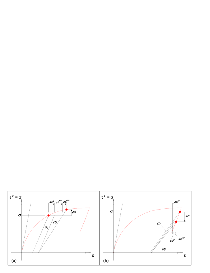
Figure 2: The increment $de_{p}$ of the energy dissipated by plastic strain (1) and the increment $de_{D}$ of the energy dissipated by damage (2). The increments of the elastic and plastic strain as well as of the stress are also schematically illustrated for a) the loading phase; and b) the unloading phase.

The two scalar quantities $\dot{e}_{p}$ and $\dot{e}_{D}$ respectively define the rate of energy per unit volume dissipated by plasticity-related phenomena and by damage phenomena; see Figure 2. Their sum $\dot{e}=\dot{e}_{p}+\dot{e}_{D}$ is the rate of the total dissipated energy per unit volume and coincides with the intrinsic dissipation $\Phi_{1}$. The restrictions imposed by these two inequalities are more severe than the original unique inequality of Clausius-Duhem (15). However, they are usually adopted as basic thermodynamic criterion for the formulation of plasticity models with damage (Lemaitre and Chaboche,, 1990). This assumption will be adopted hereafter. Taking into account (17), the pseudo-potential is supposed to split into two pseudo-potentials $\phi_{D}$ and $\phi_{p}$, respectively related to damage and plastic flow:

$$\phi\left(\mbox{\boldmath$\dot{\varepsilon}$}^{p^{\prime}},\dot{\zeta}^{\prime},\dot{D}^{\prime};\mathbf{v};\mbox{\boldmath$\rho$}\right)=\phi_{D}\left(\dot{D}^{\prime};\mathbf{v};\mbox{\boldmath$\rho$}\right)+\phi_{p}\left(\mbox{\boldmath$\dot{\varepsilon}$}^{p^{\prime}},\dot{\zeta}^{\prime};\mathbf{v};\mbox{\boldmath$\rho$}\right)$$ (18)

In the following sections, the Helmholtz free energy, the pseudo-potentials $\phi_{D}$ and $\phi_{p}$, as well as their Legendre-Fenchel transforms (Rockafellar,, 1969), are formulated for the endochronic model with damage (7).

3.1 The Helmholtz free energy

According to (10), for the DD-EC models one has the following Helmholtz free energy:

$$\Psi\left(\mathbf{v}\right)=\psi\left(\mathbf{v}\right)+\mathbb{I}_{\mathbb{H}}=\left(1-D\right)\frac{1}{2}\left(\mbox{\boldmath$\varepsilon-\varepsilon$}^{p}\right)\mathbf{:C:}\left(\mbox{\boldmath$\varepsilon-\varepsilon$}^{p}\right)+\mathbb{I}_{\mathbb{H}}$$ (19)

In this paper, two cases are considered:

$$\mathbb{H}=\left\{\begin{array}[]{l}\left(\mbox{\boldmath$\varepsilon,\varepsilon$}^{p},\zeta,D\right)\ \ \text{such\ that \ \ }D\geq 0,\ D\leq 1\\ \text{and \ \ }\left(1-D\right)^{s}R\left(\tilde{\mathbf{v}},\mbox{\boldmath$\rho$}\right)-r_{0}\leq 0\end{array}\right\}$$ (20)

where $s$ and $r_{0}$ are positive parameters; $\tilde{\mathbf{v}}=\left(\mbox{\boldmath$\varepsilon,\varepsilon$}^{p},\zeta\right)$ collects all state variables except $D$ and $R=R\left(\tilde{\mathbf{v}},\mbox{\boldmath$\rho$}\right)$ is a non-negative function called source of damage. The first two conditions on $D$ impose the minimum and the maximum values for this variable. As it will be seen, the third condition in (20) is strictly related to the definition of the damage limit surface. The second case is characterized by a different assumption:

$$\mathbb{H}=\left\{\left(\mbox{\boldmath$\varepsilon,\varepsilon$}^{p},\zeta,D\right)\ \ \text{such\ that \ }D\geq 0,\ D\leq 1\right\}$$ (21)

where only the two basic inequalities on $D$ are retained.

Making use of (14), (19), (20) and of the pseudo-potential (25), i.e. the Definition 1 of $\phi_{D}$ given in the following section, it is possible to prove that the assumption $\mathbf{q}^{ndr}=\mathbf{0}$ is admissible. The same holds for the model defined by (19),(21) and (34) (Definition 2 of $\phi_{D}$). For brevity, the details of this proof, are omitted. As a result, the non-dissipative thermodynamic forces fulfill the following relationships:

$$\begin{array}[]{l}\mbox{\boldmath$\sigma$}^{nd}=\frac{\partial\psi}{\partial\mbox{\boldmath$\varepsilon$}}=\left(1-D\right)\text{ }\mathbf{C:}\left(\mbox{\boldmath$\varepsilon-\varepsilon$}^{p}\right)=\mbox{\boldmath$\sigma$}-\mbox{\boldmath$\sigma$}^{d}=\mbox{\boldmath$\sigma$}\\ \mbox{\boldmath$\tau$}^{nd}=\frac{\partial\psi}{\partial\mbox{\boldmath$\varepsilon$}^{p}}=\mathbf{-}\left(1-D\right)\text{ }\mathbf{C:}\left(\mbox{\boldmath$\varepsilon-\varepsilon$}^{p}\right)=-\mbox{\boldmath$\tau$}^{d}\\ R^{nd}=\frac{\partial\psi}{\partial\zeta}=0=-R^{d}\\ Y^{nd}=\frac{\partial\psi}{\partial D}=-\frac{1}{2}\left(\mbox{\boldmath$\varepsilon-\varepsilon$}^{p}\right)\mathbf{:C:}\left(\mbox{\boldmath$\varepsilon-\varepsilon$}^{p}\right)=-Y^{d}\end{array}$$ (22)

Moreover using (22) and supposing $D<1$, the energy dissipation rate reads

$$\begin{array}[]{l}\dot{e}=\dot{e}_{p}+\dot{e}_{D}=\mbox{\boldmath$\sigma$}:\mbox{\boldmath$\dot{\varepsilon}$}^{p}+\frac{1}{2}\mbox{\boldmath$\sigma$}:\frac{\mathbf{C}^{-1}:\mbox{\boldmath$\sigma$}}{\left(1-D\right)^{2}}\dot{D}\\ =dev\left(\mbox{\boldmath$\sigma$}\right):dev\left(\mbox{\boldmath$\dot{\varepsilon}$}^{p}\right)+\frac{tr\left(\sigma\right)}{3}tr\left(\mbox{\boldmath$\dot{\varepsilon}$}^{p}\right)+\frac{1}{2}\left(\frac{dev\left(\sigma\right)\mathbf{:}dev\left(\sigma\right)}{2G}\mathbf{+}\frac{\left(tr\left(\mathbf{\sigma}\right)\right)^{2}}{9K}\right)\text{ }\frac{\dot{D}}{\left(1-D\right)^{2}}\end{array}$$ (23)

Taking the time-derivative of (22)₁ and recalling that no viscous effect is considered ($\mbox{\boldmath$\sigma$}^{d}=\mathbf{0}$), one obtains

$$\mbox{\boldmath$\dot{\varepsilon}$}=\mbox{\boldmath$\dot{\varepsilon}$}^{p}+\mbox{\boldmath$\dot{\varepsilon}$}^{e}=\mbox{\boldmath$\dot{\varepsilon}$}^{p}+\mathbf{C}^{-1}:\frac{\mbox{\boldmath$\dot{\sigma}$}}{1-D}+\mathbf{C}^{-1}:\frac{\mbox{\boldmath$\sigma$}\dot{D}}{\left(1-D\right)^{2}}:=\mbox{\boldmath$\dot{\varepsilon}$}^{p}+\mbox{\boldmath$\dot{\varepsilon}$}^{e,\sigma}+\mbox{\boldmath$\dot{\varepsilon}$}^{e,D}$$ (24)

where $\mbox{\boldmath$\dot{\varepsilon}$}^{e,\sigma}$ is an elastic strain flow at constant damage and $\mbox{\boldmath$\dot{\varepsilon}$}^{e,D}$ is an elastic strain flow at constant stress. It follows that $\dot{e}_{D}=1/2\left(\mbox{\boldmath$\sigma$}:\mbox{\boldmath$\dot{\varepsilon}$}^{e,D}\right)$. Note that in general the endochronic theory may present non-zero energy rates $\dot{e}_{p}$ and $\dot{e}_{D}$ also during unloading phases; see Figure 2b in this respect.

3.2 The pseudo-potential for the damage flow

The formalism of the loading function $f_{D}$, as well as the pseudo-potential $\phi_{D}^{\ast}=\mathbb{I}_{f_{D}\leq 0}$ , can be used to express the damage evolution (Lemaitre and Chaboche,, 1990; Salari et al.,, 2004; Nedjar,, 2001; Frémond,, 2002). We present herein a well-known damage evolution rule by using both pseudo-potentials $\phi_{D}$ and its dual $\phi_{D}^{\ast}$. Then, a discussion is done about a novel pseudo-potential leading to a damage evolution where $\dot{D}$ may be different from 0 also during unloading phases. In detail, the main difference between the two cases is related to the role of the damage limit surface. Standard damage evolution rules, viz. Definition 1, are characterized by the possibility for the actual state point to be inside the damage domain delimited by this limit surface; in this situation and in particular during unloading phases, damage increments are null. Conversely, in the damage evolution which we propose here, i.e. Definition 2, the present state point is forced to be always on the damage limit surface also during unloading phases.

3.2.1 Definition 1 of $\phi_{D}$

Let us begin with the following pseudo-potential, associated with the Helmholtz free energy (19)-(20):

$$\phi_{D}\left(\dot{D}^{\prime};\mathbf{v};\mbox{\boldmath$\rho$}\right)=\left[\frac{1}{2}\left(\mbox{\boldmath$\varepsilon-\varepsilon$}^{p}\right):\mathbf{C:}\left(\mbox{\boldmath$\varepsilon-\varepsilon$}^{p}\right)-\left(1-D\right)^{s}R\left(\tilde{\mathbf{v}},\mbox{\boldmath$\rho$}\right)+r_{0}\right]\text{ }\dot{D}^{\prime}+\mathbb{I}_{\mathbb{D}_{D}}\left(\dot{D}^{\prime}\right)$$ (25)

and

$$\mathbb{D}_{D}=\left\{\dot{D}^{\prime}\text{ such that }\dot{D}^{\prime}\geq 0\right\}$$ (26)

The pseudo-potential $\phi_{D}$ is the sum of a regular part, proportional to $\dot{D}^{\prime}$ and of the indicator function $\mathbb{I}_{\mathbb{D}_{D}}$. The term multiplying $\dot{D}^{\prime}$ in the regular part of $\phi_{D}$ is always non-negative, by virtue of the third condition defining $\mathbb{H}$ in (20). The regular part of $\phi_{D}$, considered for the actual flow $\dot{D}^{\prime}=\dot{D}$, represents the rate of dissipated energy $\dot{e}_{D}$. (25)-(26) allow a large number of standard damage evolution rules to be represented, according to the specific definition of $R\left(\tilde{\mathbf{v}},\mbox{\boldmath$\rho$}\right)$. An interesting example is

$$R=R\left(\mbox{\boldmath$\varepsilon$}\right)=\frac{1}{2}\left(2G\mbox{\boldmath$\varepsilon$}^{e,+}:\mbox{\boldmath$\varepsilon$}^{e,+}+\lambda\left(\left[tr\left(\mbox{\boldmath$\varepsilon$}^{e}\right)\right]^{+}\right)^{2}\right)$$ (27)

where $\lambda=K-2G/3$ is the Lamé constant. For a scalar $x$, $\left[x\right]^{+}:=\left\langle x\right\rangle$, where $\left\langle{}\right\rangle$ are the McCauley brackets. The positive part $\mbox{\boldmath$\varepsilon$}^{e,+}$ of the tensor $\mbox{\boldmath$\varepsilon$}^{e}$ is obtained after diagonalisation. Other definitions for $R$ can be adopted; see, among others, Nedjar, (2001) and Salari et al., (2004).

In order to derive the damage flow, it is convenient to consider the Legendre-Fenchel transform of $\phi_{D}$, which reads:

$$\begin{array}[]{l}\phi_{D}^{\ast}\left(Y^{d^{\prime}};\mathbf{v};\mbox{\boldmath$\rho$}\right)=\sup_{\dot{D}^{\prime}\in\mathbb{D}_{D}}\left[\left(Y^{d^{\prime}}-\frac{1}{2}\left(\mbox{\boldmath$\varepsilon-\varepsilon$}^{p}\right):\mathbf{C:}\left(\mbox{\boldmath$\varepsilon-\varepsilon$}^{p}\right)+\left(1-D\right)^{s}R\left(\tilde{\mathbf{v}},\mbox{\boldmath$\rho$}\right)-r_{0}\right)\dot{D}^{\prime}\right]\\ =\mathbb{I}_{\mathbb{E}_{D}}\left(Y^{d^{\prime}};\mathbf{v};\mbox{\boldmath$\rho$}\right)\end{array}$$ (28)

where $\mathbb{E}_{D}\mathbb{=}\left\{Y^{d^{\prime}}\text{ such that \ \ }f_{D}\left(Y^{d^{\prime}};\mathbf{v};\mbox{\boldmath$\rho$}\right)\leq 0\right\}$ is the damage loading domain and the corresponding loading function is:

$$f_{D}\left(Y^{d^{\prime}};\mathbf{v};\mbox{\boldmath$\rho$}\right)=Y^{d^{\prime}}-\frac{1}{2}\left(\mbox{\boldmath$\varepsilon-\varepsilon$}^{p}\right):\mathbf{\ C:}\left(\mbox{\boldmath$\varepsilon-\varepsilon$}^{p}\right)+\left(1-D\right)^{s}R\left(\tilde{\mathbf{v}},\mbox{\boldmath$\rho$}\right)-r_{0}:=Y^{d^{\prime}}-Y_{\max}^{d^{\prime}}$$ (29)

By using the normality assumption, the relevant damage flow rule reads

$$\begin{array}[]{l}\dot{D}=\dot{\lambda}_{D}\frac{\partial f_{D}\left(Y^{d}\right)}{\partial Y^{d^{\prime}}}=\dot{\lambda}_{D}\\ \text{with }f_{D}\left(Y^{d};\mathbf{v};\mbox{\boldmath$\rho$}\right)\dot{\lambda}_{D}=0,\text{ \ \ }\dot{\lambda}_{D}\geq 0,\text{ \ \ \ \ }f_{D}\left(Y^{d};\mathbf{v};\mbox{\boldmath$\rho$}\right)\leq 0.\end{array}$$ (30)

At the actual state, it holds $Y^{d^{\prime}}=Y^{d}=-Y^{nd}$, and therefore:

$$f_{D}=f_{D}\left(Y^{d};\mathbf{v};\mbox{\boldmath$\rho$}\right)=\left(1-D\right)^{s}R\left(\tilde{\mathbf{v}},\mbox{\boldmath$\rho$}\right)-r_{0}\leq 0,$$ (31)

which is the damage limit surface, but also is one of the conditions defining the set $\mathbb{H}$. It becomes evident that the positive constant $r_{0}$ is the initial damage threshold. The Kuhn-Tucker conditions state that $f_{D}<0$ implies no damage increment, while $f_{D}\left(Y^{d};\mathbf{v};\mbox{\boldmath$\rho$}\right)=0$ corresponds to a damage increment which can be computed by enforcing the consistency condition:

$$\dot{f}_{D}=\left(1-D\right)^{s}\left(\frac{\partial R\left(\tilde{\mathbf{v}},\mbox{\boldmath$\rho$}\right)}{\partial\tilde{\mathbf{v}}}\mathbf{\dot{\tilde{v}}+}\frac{\partial R\left(\tilde{\mathbf{v}},\mbox{\boldmath$\rho$}\right)}{\partial\mbox{\boldmath$\rho$}}\mbox{\boldmath$\dot{\rho}$}\right)-R\left(\tilde{\mathbf{v}},\mbox{\boldmath$\rho$}\right)s\left(1-D\right)^{s-1}\dot{D}=0$$ (32)

leading to the explicit expression of the damage flow

$$\dot{D}=H\left(f_{D}\right)\left(\frac{\partial R\left(\tilde{\mathbf{v}},\mbox{\boldmath$\rho$}\right)}{\partial\tilde{\mathbf{v}}}\mathbf{\dot{\tilde{v}}+}\frac{\partial R\left(\tilde{\mathbf{v}},\mbox{\boldmath$\rho$}\right)}{\partial\mbox{\boldmath$\rho$}}\mbox{\boldmath$\dot{\rho}$}\right)\frac{1-D}{s\text{ }R\left(\tilde{\mathbf{v}},\mbox{\boldmath$\rho$}\right)},$$ (33)

where $H$ is the Heaviside function. The presence of the Heaviside function in the damage flow definition indicates that damage increments are zero during unloading phases. Note that (33) entails that the limit condition $D=1$ is never reached.

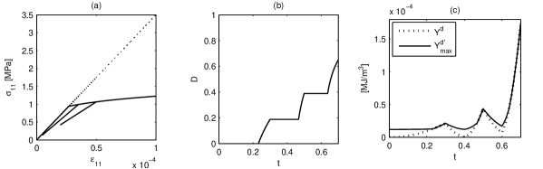
Figure 3: Elastic with damage model. Uniaxial behavior. (a) The stress-strain evolution. The dotted line indicates the effective stress $\sigma_{11}/(1-D)$. (b) The damage evolution, with the damage increasing only during loading phases. (c) Time-evolution of $Y^{d}$, i.e. the actual value of the thermodynamic force $Y^{d^{\prime}}$, and of $Y^{d^{\prime}}_{max}$, i.e. the upper bound of $Y^{d^{\prime}}$ defined in (29).

Figure 3 illustrates some loading-unloading cycles of an elastic with damage model ($\dot{\zeta}=0$). The uniaxial stress is considered, viz. all the components of the Cauchy tensor are supposed to be null, except $\sigma_{11}$. The parameter values represent a hypothetical material for which the Young modulus $E=35000$ $MPa$ and the Poisson ratio $\nu=0.18$ are close to those of concrete; damage is defined by (20) and (27), with $s=2.5$ and $r_{0}=1.2e-05$ $MJ/m^{3}$; see also the numerical examples in Nedjar, (2001). Together with the stress-strain and damage evolution of this model, Figure 3 depicts the evolution of $Y^{d}=1/2\left(\mbox{\boldmath$\varepsilon-\varepsilon$}^{p}\right):\mathbf{C:}\left(\mbox{\boldmath$\varepsilon-\varepsilon$ }^{p}\right)$, i.e. the actual value of $Y^{d^{\prime}}$, and of the quantity $Y_{\max}^{d^{\prime}}=1/2\left(\mbox{\boldmath$\varepsilon-\varepsilon$ }^{p}\right):\mathbf{C:}\left(\mbox{\boldmath$\varepsilon-\varepsilon$ }^{p}\right)+r_{0}-(1-D)^{s}R\left(\mbox{\boldmath$\varepsilon$}\right)$, defining the upper limit of $Y^{d^{\prime}}$ according to (29). When these two curves are superposed, the damage increases.

3.2.2 Definition 2 of $\phi_{D}$

Unfortunately, a definition of $\dot{D}$ of the type (33), deriving from the pseudo-potential (25) and the condition (20), is not able to represent the case of damage increasing during both loading and unloading phases, owing to the condition $f_{D}\leq 0$. We recall that the case of damage increasing during unloading may occur in Bouc-Wen models with stiffness degradation (Erlicher and Bursi,, 2007). A damage pseudo-potential, simpler than (25), is more suited:

$$\phi_{D}\left(\dot{D}^{\prime};\mathbf{v}\right)=\left[\frac{1}{2}\left(\mbox{\boldmath$\varepsilon-\varepsilon$ }^{p}\right):\mathbf{C:}\left(\mbox{\boldmath$\varepsilon-\varepsilon$}^{p}\right)\right]\text{ }\dot{D}^{\prime}+\mathbb{I}_{\mathbb{D}_{D}}\left(\dot{D}^{\prime}\right)$$ (34)

with $\mathbb{D}_{D}$ still provided by (26) and with the conditions on the damage state variable defined in (21). As already observed, it is possible to prove that the assumption $\mathbf{q}^{ndr}=\mathbf{0}$ is admissible also for this Definition 2 of the damage pseudo-potential. The dual pseudo-potential becomes $\phi_{D}^{\ast}\left(Y^{d^{\prime}};\mathbf{v}\right)=\mathbb{I}_{\mathbb{E}_{D}}\left(Y^{d^{\prime}};\mathbf{\ \ \ v}\right)$ where $\mathbb{E}_{D}\mathbb{=}\left\{Y^{d^{\prime}}\text{ such that \ }f_{D}\left(Y^{d^{\prime}};\mathbf{v}\right)\leq 0\right\}$ is the corresponding damage loading domain, with the damage loading function

$$f_{D}\left(Y^{d^{\prime}};\mathbf{v}\right)=Y^{d^{\prime}}-\frac{1}{2}\left(\mbox{\boldmath$\varepsilon-\varepsilon$ }^{p}\right):\mathbf{C:}\left(\mbox{\boldmath$\varepsilon-\varepsilon$ }^{p}\right):=Y^{d^{\prime}}-Y^{d^{\prime}}_{max}$$ (35)

At the actual state, $Y^{d^{\prime}}=Y^{d}=-Y^{nd}$ and therefore $f_{D}\left(Y^{d};\mathbf{v}\right)=0$ at every instant. Therefore, the relationships (30) reduce to $\dot{D}=\dot{\lambda}_{D}\partial f_{D}/\partial Y^{d^{\prime}}=\dot{\lambda}_{D}$, with $\dot{\lambda}_{D}\geq 0$. Moreover, $\dot{D}=\dot{\lambda}_{D}$ can no longer be computed by the consistency condition, fulfilled as an identity at every instant. Hence, it must be rather defined by an additional condition. Any definition ensuring rate-independence, consistent with (21) and fulfilling $\dot{D}=\dot{\lambda}_{D}\geq 0$ is admissible, even though is characterized by non-zero damage increments during unloading phases.

3.3 The pseudo-potential for the plastic flow

The usual method to define associated plastic flows is based on the notion of loading function, indicated here by $f_{p}$, as well as on the normality assumption. Another equivalent formalism is based on the use of the dual pseudo-potential $\phi_{p}^{\ast}=\mathbb{I}_{f_{p}\leq 0}$ (Moreau,, 1970). A third way to formulate plasticity models is based on the pseudo-potential $\phi_{p}$, Legendre-Fenchel conjugate of $\phi_{p}^{\ast}$ (Frémond,, 2002; Ziegler and Wehrli,, 1987; Houlsby and Puzrin,, 2000; Erlicher and Point,, 2006). The advantage of using the formalism based on $f_{p}$ (or $\phi_{p}^{\ast}=\mathbb{I}_{f_{p}\leq 0}$) is essentially simplicity. Moreover, when a non-associated flow is to be defined, the simple introduction of a second function $g_{p}$ called plastic potential matches this purpose. Nonetheless, for some non-classical plasticity theories, like endochronic theory and generalized plasticity (Lubliner et al.,, 1993), it is not straightforward to provide a proper definition of the loading function $f_{p}$. It was proved by Erlicher and Point, (2006) that for these plasticity theories (without damage) a way to define the loading function is to start from the definition of the pseudo-potential $\phi_{p}$, to compute the dual potential $\phi_{p}^{\ast}$ and then to derive $f_{p}$. An important point is the additional dependence of $\phi_{p}$, and therefore of $\phi_{p}^{\ast}$ and the loading function too, on the state variables. This dependence is only optional for standard plasticity theories but is essential both for the endochronic theory and the generalized plasticity. Moreover, we notice that some models with non-associated flow also admit a representation based on the definition of a suited pseudo-potential $\phi_{p}$, depending on state variables. The example of a non-associated Drucker-Prager model can be found in Erlicher and Point, (2005); in particular, it is shown that a suited pseudo-potential $\phi_{p}$ leads to a modified loading function which plays both roles of the traditional loading function and of the plastic potential.

For the endochronic models with damage, the plasticity pseudo-potential is defined as follows:

$$\phi_{p}\left(\mbox{\boldmath$\dot{\varepsilon}$}^{p^{\prime}},\dot{\zeta}^{\prime};\mathbf{v};\mbox{\boldmath$\rho$ }\right)=\left(1-D\right)\frac{\left\|dev\left(\mathbf{C:}\left(\mbox{\boldmath$\varepsilon-\varepsilon$}^{p}\right)\right)\right\|^{2}}{2G/\beta}\frac{\dot{\zeta}^{\prime}}{g\left(\mathbf{v},\mbox{\boldmath$\rho$ }\right)}+\mathbb{I}_{\mathbb{D}}\left(\mbox{\boldmath$\dot{\varepsilon}$}^{p^{\prime}},\dot{\zeta}^{\prime};\mathbf{v};\mbox{\boldmath$\rho$ }\right)$$ (36)

where $\mathbb{I}_{\mathbb{D}}$ is the indicator function of the convex set

$$\mathbb{D=}\left\{\begin{array}[]{l}\left(\mbox{\boldmath$\dot{\varepsilon}$}^{p^{\prime}},\dot{\zeta}^{\prime}\right)\text{ such that }\\ tr\left(\mbox{\boldmath$\dot{\varepsilon}$}^{p^{\prime}}\right)=0,\text{ \ }\dot{\zeta}^{\prime}\geq 0\text{ and }\\ \mbox{\boldmath$\dot{\varepsilon}$}^{p^{\prime}}=\frac{dev\left(\mathbf{C:}\left(\mbox{\boldmath$\varepsilon-\varepsilon$}^{p}\right)\right)}{2G/\beta}\frac{\dot{\zeta}^{\prime}}{g\left(\mathbf{v},\rho\right)}\end{array}\right\}$$ (37)

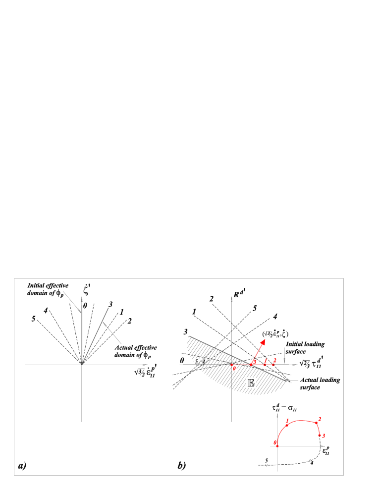
Figure 4: Endochronic model with damage in the uniaxial stress regime. (a) Several configurations of the effective domain $\mathbb{D}$ of the pseudo-potential $\phi_{p}$. (b) Corresponding configurations of the loading domain $\mathbb{E}$, associated with the loading function $f_{p}$. The actual stress point always occurs at $R^{d^{\prime}}=R^{d}=0$ and, at this point, the flows $\dot{\mbox{\boldmath$\varepsilon$}}^{p}$ and $\dot{\zeta}$ are defined by the normality condition.

(see Figure 4a). The first equality in $\mathbb{D}$ imposes the plastic incompressibility of the flow. Moreover, since $D$ is supposed to be less or equal to one and $g=g\left(\mathbf{v},\mbox{\boldmath$\rho$}\right)$, the hardening-softening function, is positive by assumption, the second condition in $\mathbb{D}$ ensures the positivity of $\phi_{p}$. Therefore, the standard properties of $\phi_{p}$, viz. non-negativity, convexity and positive homogeneity of order 1, are matched. The third condition in $\mathbb{D}$ gives the plastic flow and is consistent with (7). It can be proven that when $\mbox{\boldmath$\dot{\varepsilon}$}^{p^{\prime}}=\mbox{\boldmath$\dot{\varepsilon}$}^{p}$ and $\dot{\zeta}^{\prime}=\dot{\zeta}$, i.e. when the actual flows are considered, the first term of the sum in (36) represents the rate of energy $\dot{e}_{p}$ dissipated by the plastic flow, defined in (17) for the general case. Note that the pseudo-potential has an additional dependence on the state variables and on the past-history dependent parameters collected in $\rho$.

The dual dissipation potential $\phi_{p}^{\ast}$ is obtained by the Legendre-Fenchel transformation of $\phi_{p}$ (Rockafellar,, 1969). Since $\phi_{p}$ is positively homogeneous of order 1, then $\phi_{p}^{\ast}$ is an indicator function:

$$\begin{array}[]{l}\phi_{p}^{\ast}\left(\mbox{\boldmath$\tau$}^{d^{\prime}},R^{d^{\prime}};\mathbf{\ v};\mbox{\boldmath$\rho$}\right)=\underset{\left(\dot{\varepsilon}^{p^{\prime}},\dot{\zeta}^{\prime}\right)\in\mathbb{D}}{\sup}\left(\mbox{\boldmath$\tau$}^{d^{\prime}}:\mbox{\boldmath$\dot{\varepsilon}$}^{p^{\prime}}+R^{d^{\prime}}\dot{\zeta}^{\prime}-\phi_{p}\left(\mathbf{\dot{v}}^{\prime};\mathbf{v};\mbox{\boldmath$\rho$}\right)\right)\\ \text{ \ \ \ }=\underset{\left(\dot{\varepsilon}^{p^{\prime}},\dot{\zeta}^{\prime}\right)\in\mathbb{D}}{\sup}\left(dev\left(\mathbf{\tau}^{d^{\prime}}\right)\mathbf{:}\frac{dev\left(\mathbf{C:}\left(\mbox{\boldmath$\varepsilon-\varepsilon$}^{p}\right)\right)}{2G\text{ }g\left(\mathbf{v},\rho\right)\text{ }/\beta}\dot{\zeta}^{\prime}+R^{d^{\prime}}\dot{\zeta}^{\prime}-\left(1-D\right)\frac{\left\|dev\left(\mathbf{C:}\left(\mbox{\boldmath$\varepsilon-\varepsilon$}^{p}\right)\right)\right\|^{2}}{2Gg\left(\mathbf{v},\rho\right)/\beta}\dot{\zeta}^{\prime}\right)\\ \text{ \ \ \ }=\mathbb{I}_{\mathbb{E}}\left(\mbox{\boldmath$\tau$}^{d^{\prime}},R^{d^{\prime}};\mathbf{v};\mbox{\boldmath$\rho$}\right)\end{array}$$ (38)

The indicator function $\mathbb{I}_{\mathbb{E}}$ is associated with the convex set
$\mathbb{E=}\left\{\left(\mbox{\boldmath$\tau$}^{d^{\prime}},R^{d^{\prime}}\right)\text{ such that }f_{p}\left(\mbox{\boldmath$\tau$}^{d^{\prime}},R^{d^{\prime}};\mathbf{v};\mbox{\boldmath$\rho$}\right)\leq 0\right\}$ (see Figure 4b) with

$$f_{p}\left(\mbox{\boldmath$\tau$}^{d^{\prime}},R^{d^{\prime}};\mathbf{v};\mbox{\boldmath$\rho$}\right)=dev\left(\mbox{\boldmath$\tau$}^{d^{\prime}}\right)\mathbf{:}\frac{dev\left(\mathbf{C:}\left(\mbox{\boldmath$\varepsilon-\varepsilon$}^{p}\right)\right)}{2Gg\left(\mathbf{v},\mbox{\boldmath$\rho$}\right)/\beta}-\left(1-D\right)\frac{\left\|dev\left(\mathbf{C:}\left(\mbox{\boldmath$\varepsilon-\varepsilon$}^{p}\right)\right)\right\|^{2}}{2Gg\left(\mathbf{v},\mbox{\boldmath$\rho$}\right)/\beta}+R^{d^{\prime}}$$ (39)

The function $f_{p}$ is the loading function for an endochronic model with plastic incompressibility and with isotropic damage. It is associated with the loading domain $\mathbb{E}$. If the past-history parameter $\rho$ is a scalar equal to $e_{p}$, the plastic dissipated energy, then a work-hardening behavior is defined, in the sense that the loading function evolves with the plastic dissipated energy. A different approach to define work-hardening plasticity models was proposed by Ristinmaa, (1999).

The generalized normality conditions imposed on $\phi_{p}^{\ast}$ leads to:

$$\left\{\begin{array}[]{l}\mbox{\boldmath$\dot{\varepsilon}$}^{p}=\dot{\lambda}\frac{\partial f_{p}\left(\mathbf{\tau}^{d},R^{d};\mathbf{v};\rho\right)}{\partial\mathbf{\tau}^{d^{\prime}}}=\dot{\lambda}\frac{dev\left(\mathbf{C:}\left(\mathbf{\varepsilon-\varepsilon}^{p}\right)\right)}{2Gg\left(\mathbf{v},\rho\right)/\beta}\\ \dot{\zeta}=\dot{\lambda}\frac{\partial f_{p}\left(\mathbf{\tau}^{d},R^{d};\mathbf{v};\rho\right)}{\partial R^{d^{\prime}}}=\dot{\lambda}\\ \dot{\lambda}f_{p}\left(\mbox{\boldmath$\tau$}^{d},R^{d};\mathbf{v};\mbox{\boldmath$\rho$ }\right)=0\text{ \ \ \ \ \ \ \ }f_{p}\left(\mbox{\boldmath$\tau$}^{d},R^{d};\mathbf{v};\mbox{\boldmath$\rho$ }\right)\leq 0,\text{ \ \ \ \ \ \ }\dot{\lambda}\geq 0\end{array}\right.$$ (40)

where the last three inequalities are the Kuhn-Tucker conditions. The plastic flow defined in (7) is retrieved. Note that the derivatives are taken with respect to the generic variables $\mbox{\boldmath$\tau$}^{d^{\prime}}$ and $R^{d^{\prime}}$, but they are computed at the present state $\mbox{\boldmath$\tau$}^{d^{\prime}}=\mbox{\boldmath$\tau$}^{d}$ and $R^{d^{\prime}}\mathbf{=}R^{d}$. In summary, the usual notions of plastic multiplier and loading surface have been defined for an endochronic model with damage. This kind of thermodynamic formulation for endochronic models is quite innovative and has been first presented in Erlicher and Point, (2006), for the case of no damage. As was pointed out in that paper, an important property characterizing endochronic models is the fact that at the actual state, the loading function $f_{p}$ is always zero: for this reason, the consistency condition $\dot{f}_{p}=0$ is always fulfilled as an identity and cannot be used to compute the plastic multiplier $\dot{\lambda}$. This is also true in this case, where the actual state is $\left(\mbox{\boldmath$\tau$}^{d},R^{d}\right)=\left(\left(1-D\right)\mathbf{C:}\left(\mbox{\boldmath$\varepsilon-\varepsilon$}^{p}\right),0\right).$ As a result, the Kuhn-Tucker conditions reduce to $\dot{\lambda}=\dot{\zeta}\geq 0$, where $\dot{\zeta}$ is the flow of the internal variable associated with $R^{d}$ and, using the language of the endochronic theory, is also the flow of the intrinsic time measure; it can be freely defined, provided that it is non-negative and that rate-independence is guaranteed. As already observed, the standard choice is $\dot{\zeta}=\left\|dev\left(\mbox{\boldmath$\dot{\varepsilon}$}\right)\right\|$.

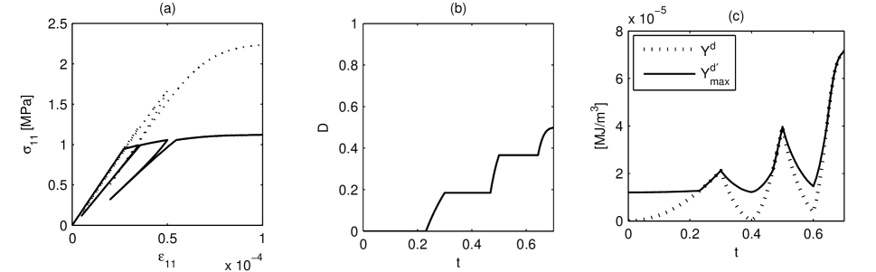
Figure 5: Uniaxial behavior of an endochronic plasticity model with damage (Definition 1). (a) The stress-strain evolution. The dotted line indicates the effective stress $\sigma_{11}/(1-D)$. (b) Damage evolution. (c) See Figure 3c.

Figure 5 illustrates an example of uniaxial behavior of an endochronic plasticity model with damage. The parameters of the elastic phase and of damage (Definition 1) are the same as those of Figure 3. In addition, $g=1$, $\dot{\zeta}$ is given by ( 9) with $n=5$ , $\beta=2834.9$ $MPa^{1-n}$ and $\gamma/\beta=-0.5$ ; as a result, $\sigma_{u}=\left(2G/\left(\beta+\gamma\right)\right)^{1/n}=2.25\ast\sqrt{2/3}=1.8371$ $MPa$, where $\sigma_{u}$ is the upper limit of $\|dev\left(\mbox{\boldmath$\tau$}^{d}/\left(1-D\right)\right)\|=\|dev\left(\mbox{\boldmath$\sigma$}/\left(1-D\right)\right)\|=\sqrt{2/3}\ \sigma_{11}/\left(1-D\right)$ when $g=1$.

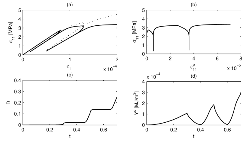
Figure 6: Uniaxial behavior of an endochronic plasticity model with damage (Definition 2). (a) The stress-strain evolution. The dotted line indicates the effective stress $\sigma_{11}/(1-D)$. (b) The stress as function of the plastic strain. Observe that the plastic strain increases during unloading phases. (c) The damage evolution, with damage slightly increasing also during unloading phases. (d) Evolution of $Y^{d}$ vs. time.

In the example of Figure 6, the damage is defined by the rule $D=1-1/\left(1+c_{\eta}e_{p}\right)$, with $c_{\eta}=1500$ $m^{3}MJ^{-1}$ (Definition 2). The parameter $c_{\eta}$ indicates the sensitivity of damage to the energy $e_{p}$ dissipated by plasticity. If $c_{\eta}$ is large, the damage increment at a given $e_{p}$-value is larger than in the case of small $c_{\eta}$. The Young modulus and the Poisson ratio are the same as in the previous figures. The parameters defining the intrinsic time flow (9) are: $n=15$, $\beta=16.1846$ $MPa^{1-n}$ and $\gamma/\beta=-0.8$ ; as a result, $\sigma_{u}=\left(2G/\left(\beta+\gamma\right)\right)^{1/n}=2.25\ast\sqrt{2/3}=1.8371$ $MPa$. Moreover, the hardening function is defined as $g=\left(1+\|dev\left(\mbox{\boldmath$\varepsilon$}\left(t^{\prime}\right)\right)\|_{max_{t^{\prime}\in[0,t]}}/\varepsilon_{u}\right)^{n}$, where $t$ is the present time and $\varepsilon_{u}=0.0002$. Figure 6d depicts the evolution of $Y^{d}=1/2\left(\mbox{\boldmath$\varepsilon-\varepsilon$ }^{p}\right):\mathbf{C:}\left(\mbox{\boldmath$\varepsilon-\varepsilon$}^{p}\right)$, i.e. the actual value of $Y^{d^{\prime}}$. According to (35), this quantity is also equal to $Y_{\max}^{d^{\prime}}$, which is the upper limit of $Y^{d^{\prime}}$. The typical endochronic behavior with plastic strains increasing during unloading phases is highlighted in Figure 6b. As a result, owing to the damage rule depending on the dissipated plastic energy, also the damage slightly increases during the unloading phases: observe the damage evolution after t=0.3 and t=0.5, which are the instants where unloading phases begin.

4 A brief discussion about stability and uniqueness

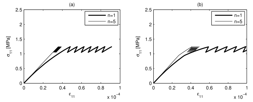
Figure 7: Strain accumulation, uniaxial behavior with stress varying between $1.05$ and $1.24$ $MPa$. (a) Endochronic model without damage, with the intrinsic time (4). (b) Endochronic model with damage, with the intrinsic time (9) and the damage evolution given by (27) and (33), with $r_{0}=0.000012$ and $s=6$.

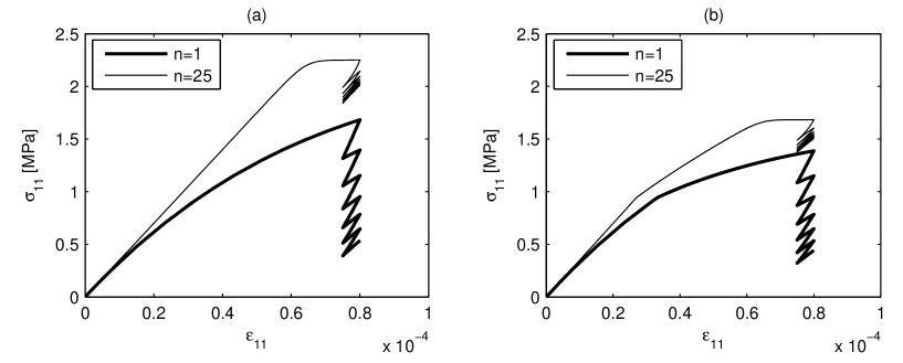
Figure 8: Stress relaxation, uniaxial behavior with strain varying between 0.000075 and 0.00008. (a) Endochronic model without damage. (b) Endochronic model with damage, with the same damage parameters as in Figure 7b.

It is well-known that standard endochronic models violate the Drucker’s postulate and the Ilyushin’s postulate, see e.g. (Sandler,, 1978). As a result, inelastic strains may continuously increase if a cyclic stress of constant and arbitrarily small amplitude is imposed around a given static stress (Figure 7a). Dually, a stress relaxation occurs when cycling straining is imposed (Figure 8a). The parameters used for the numerical simulations of Figures 7 and 8 are: $E=35000$ $MPa$, $\nu=0.18$, $g=1$, $\gamma/\beta=-0.5$, while $\beta$ has a value such that $\left(2G/\left(\beta+\gamma\right)\right)^{1/n}=1.8371$ $MPa$, for the given $n$ values used in the figures. The strain accumulation entails a violation of a Lyapunov-type stability condition. For this reason, endochronic theory have been repeatedly criticized in the past years. However, Bažant, (1978, p.705) showed that endochronic models do fulfil some weaker physically motivated stability conditions. Moreover, there are materials that are stable in the Drucker’s sense and others that are not. Hence, for these materials, a proper model cannot fulfil the postulate of Drucker. All the aspects concerning this subject have been explored in detail in the previously cited references (Sandler,, 1978; Bažant,, 1978) for endochronic models without damage. A detailed analysis for the case of models with damage would deserve further studies, but this is beyond the purposes of this paper. Figures 7a and 8a simply show the influence of the parameter $n$ on the strain accumulation and the stress relaxation for an endochronic model without damage. When $n$ tends to infinity, a plastic behavior of Prandtl-Reuss type is retrieved, where neither strain accumulation nor stress relaxation occur. Figures 7b and 8b concern models with damage.

Another important topic concerning plasticity and/or damage models is the loss of uniqueness due to strain-softening; see e.g. (Jirásek and Bažant,, 2002). An exhaustive treatment of this subject for endochronic models with damage requires further analyses. However, for illustrative purposes, a simple analytical study of a uniaxial model is presented hereafter. Let $\sigma$, $\varepsilon$ and $\varepsilon^{p}$ be the stress, the total strain and the plastic strain in the axial direction, respectively. Then, the uniaxial behavior can be represented by the following law: $\sigma=\left(1-D\right)E\left(\varepsilon-\varepsilon^{p}\right)=\left(1-D\right)E\varepsilon^{e}$, where $E$ is the Young modulus. The incremental form reads

$$d\sigma=\left(1-D\right)E\left(d\varepsilon-d\varepsilon^{p}\right)-\sigma\frac{dD}{1-D}=\left(1-D\right)Ed\varepsilon-\beta\sigma\frac{d\zeta}{g}-\sigma\frac{dD}{1-D}$$ (41)

where the intrinsic time increment is

$$d\zeta=\left(1+\frac{\gamma}{\beta}sign\left(\sigma d\varepsilon\right)\right)\left|\sigma\right|^{n-1}\left(1-D\right)^{1-n}\left|d\varepsilon\right|$$ (42)

and the damage increment writes

$$dD=H\left(f_{D}\right)\frac{dR}{d\varepsilon^{e}}d\varepsilon^{e}\frac{1-D}{s\text{ }R\left(\varepsilon^{e}\right)}$$ (43)

with $R\left(\varepsilon^{e}\right)=E\left\langle\varepsilon^{e}\right\rangle^{2}/2$ and $f_{D}=\left(1-D\right)^{s}R\left(\varepsilon^{e}\right)-r_{0}\leq 0$. Assume $\sigma>0$ and $d\varepsilon>0$ (loading); the case $\sigma<0$, $d\varepsilon<0$ is analogous. Then, the condition to avoid strain-softening is

$$d\sigma\geq 0$$ (44)

The generic damage increment when $f_{D}=0$ is given by

$$dD=\frac{2}{s}\frac{1-D}{\varepsilon^{e}}d\varepsilon^{e}=\frac{2}{s}E\frac{\left(1-D\right)^{2}}{\sigma}\left(d\varepsilon-d\varepsilon^{p}\right)$$

Moreover, from (41) one has $d\varepsilon^{p}=\beta\sigma d\zeta/\left[E\left(1-D\right)g\right].$ Hence, the condition (44) assumes the following form

$$\left(\left(1-D\right)Ed\varepsilon-\beta\sigma\frac{d\zeta}{g}\right)\left(1-\frac{2}{s}\right)\geq 0$$ (45)

The first factor is always positive provided that $g\geq 1$. This can be proven using the definition of $d\zeta$ given in (42) with $\sigma>0,d\varepsilon>0$ and observing that the non-negativity of the first factor in (45) is equivalent to the condition $\sigma/\left(1-D\right)\leq\left(E/\left(\beta+\gamma\right)\right)^{1/n}\left(g\right)^{1/n}=\sigma_{y}\left(g\right)^{1/n}$, stating that the effective stress is always less or equal than the bounding axial stress $\sigma_{y}$, modified by the hardening function $g$. If $g\geq 1$, this inequality is always strictly fulfilled. Hence, strain-softening can be avoided if $s\geq 2$ . The same result can be obtained using the tensor expressions (7), (9), (27) and (33) and imposing that all the stress components are zero except $\sigma_{11}:=\sigma$. This proof is omitted for brevity. The same condition on $s$ has been found for the case of elasticity with damage (Nedjar,, 2001). Note that $g<1$ induces strain-softening also when there is no damage. The analysis of the unloading case is not necessary, since at a given stress-strain state with $\sigma\neq 0$, the unloading stiffness is always greater than the loading one. A more complex analysis, not considered here, is needed for the multi-axial case, where the fourth-order tensor of tangential moduli for the endochronic model with damage should be computed. If strain-softening is avoided, the uniaxial behavior in what concerns the strain accumulation and the stress relaxation is analogous to that of standard endochronic models.

5 Conclusions

An extended endochronic theory with a scalar damage variable was developed, based on the postulate of strain equivalence and by using pseudo-potentials depending on state variables and on parameters related to the past history of the material. The relevant loading surfaces, for damage and for plasticity, were defined. Two different damage pseudo-potentials were discussed and a formalization of the conditions on state variables affecting the definition of damage was provided, by an additional indicator function in the Helmholtz free energy. In a companion paper (Erlicher and Bursi,, 2007) , a link between this extended endochronic theory and the Bouc-Wen type models with both strength and stiffness degradation is established. This will permit to prove the thermodynamic admissibility of these Bouc-Wen models and to highlight a constraint for the relevant stiffness degradation rules.

6 Appendix: Notations

The following symbols are used in this paper:

$\mathbf{C}=$ fourth-order elasticity tensor

$D=$ internal variable associated with isotropic damage

$e_{D}=$ energy per unit volume dissipated through damage

$e_{p}=$ energy per unit volume dissipated through plasticity

$f_{D}=$ loading function for damage

$f_{p}=$ loading function for plasticity

$G=$ shear modulus

$g=$ hardening-softening function

$H(\cdot)=$ Heaviside function

$\mathbf{I}=$ fourth-order identity tensor

$\mathbb{I}_{\mathbb{H}}=$ indicator function of the set $\mathbb{H}$

$K=$ bulk modulus

$\mathbf{q}^{d}=$ dissipative thermodynamic forces vector

$\mathbf{q}^{nd}=$ non-dissipative thermodynamic forces vector

$R^{d}=$ dissipative part of the thermodynamic force introducing isotropic hardening(softening)

$R^{nd}=$ non-dissipative part of the thermodynamic force introducing isotropic hardening(softening)

$\mathbf{v}=$ state variables vector

$Y^{d}=$ dissipative part of the thermodynamic force dual to the damage variable

$Y^{nd}=$ non-dissipative part of the thermodynamic force dual to the damage variable

$\mathbf{z}=$ hysteretic part of the stress tensor

$\beta=$ coefficient defining the plastic flow of Endochronic models

$\gamma=$ coefficient defining the plastic flow of Endochronic models

$\mbox{\boldmath$\varepsilon$}=$ total small strain tensor

$\mbox{\boldmath$\varepsilon$ }^{p}=$ plastic small strain tensor

$\zeta=$ intrinsic time measure for Endochronic models. Moreover, it is the internal variable associated with isotropic hardening/softening of Endochronic models

$\vartheta=$ intrinsic time scale for Endochronic models

$\dot{\lambda}=$ plastic multiplier

$\dot{\lambda_{D}}=$ damage multiplier

$\mu=$ hereditary kernel

$\mbox{\boldmath$\rho$}=$ history-dependent parameters vector

$\mbox{\boldmath$\sigma$}=$ Cauchy stress tensor

$\mbox{\boldmath$\sigma$}^{d}=$ dissipative part of the Cauchy stress tensor

$\mbox{\boldmath$\sigma$}^{nd}=$ non-dissipative part of the Cauchy stress tensor

$\mbox{\boldmath$\tau$}^{d}=$ dissipative part of the thermodynamic force dual to the plastic strain tensor

$\mbox{\boldmath$\tau$}^{nd}=$ non-dissipative part of the thermodynamic force dual to the plastic strain tensor

$\Phi_{1}=$ mechanical or intrinsic dissipation

$\phi=$ pseudo-potential or dissipation potential for plasticity

$\phi^{\ast}=$ dual pseudo-potential for plasticity

$\phi_{D}=$ pseudo-potential or dissipation potential for damage

$\phi_{D}^{\ast}=$ dual pseudo-potential for damage

$\Psi=$ Helmholtz free energy volume density

$\mathbf{1}=$ second-order identity tensor

$\langle\rangle$=McCauley brackets

Figure 1: Classification of Endochronic models and most relevant references. The black square indicates that a thermodynamic formulation based on a suited pseudo-potential was found for the associated group of models.

References

- Auricchio and Taylor, (1995) Auricchio, F., and Taylor, R.L. (1995). ”Two material models for cyclic plasticity: nonlinear kinematic hardening and generalized plasticity.” Int. J. Plast., 11(1), 65-98.
- Baber and Wen, (1981) Baber, T.T., and Wen, Y.-K. (1981). ”Random vibrations of hysteretic, degrading systems.” J. Engrg. Mech. Div. ASCE, 107(6), 1069-1087.
- Bažant and Bath, (1976) Bažant, Z.P., and Bath, P.D. (1976). ”Endochronic theory of inelasticity and failure of concrete.” J. Engrg. Mech. Div. ASCE, 102, 701-722.
- Bažant, (1978) Bažant, Z.P. (1978). ”Endochronic inelasticity and incremental plasticity.” Int. J. Solids Struct., 14, 691-714.
- Bouc, (1971) Bouc, R. (1971). ”Modèle mathématique d’hystérésis.” Acustica, 24, 16-25 (in French).
- Casciati, (1989) Casciati, F. (1989). ”Stochastic dynamics of hysteretic media.” Struct. Safety, 6, 259-269.
- Chow and Chen, (1992) Chow, C.L., Chen, X.F. (1992). ”An anisotropic model of damage mechanics based on endochronic theory of plasticity.” Int. J. Fracture, 55, 115-130.
- Collins and Houlsby, (1997) Collins, I.F., and Houlsby, G.T. (1997). ”Application of thermomechanical principles to the modelling of geotechnical materials.” Proc. Royal Society of London, Series A, 453, 1975–2001.
- Eisenberg and Phillips, (1971) Eisenberg, M.A., and Phillips, A. (1971). ”A theory of Plasticity with non-coincident yield and loading surfaces.” Acta Mechanica, 11, 247-260.
- Erlicher and Bursi, (2007) Erlicher, S., and Bursi, O.S. (2007). ”Bouc-Wen type models with stiffness degradation: thermodynamic analysis and applications.”, J. Engrg. Mech., accepted.
- Erlicher and Point, (2005) Erlicher, S., and Point, N. (2005). ”On the associativity of the Drucker-Prager model.” Proc. VIII Int. Conf. on Computation Plasticity COMPLAS VIII. Eds: E. Oñate, D.R.J. Owen., ECCOMAS-IACM, Barcelona, Spain.
- Erlicher and Point, (2006) Erlicher, S., and Point, N. (2006). ”Endochronic theory, non-linear kinematic hardening rule and generalized plasticity: a new interpretation based on generalized normality assumption.” Int. J. Solids Struct., 43(14-15), 4175-4200.
- Frémond, (2002) Frémond, M. (2002). Non-Smooth Thermomechanics, Springer-Verlag, Berlin.
- Houlsby and Puzrin, (2000) Houlsby, G.T., and Puzrin, A.M. (2000). ”A thermomechanical framework for constitutive models for rate-independent dissipative materials.” Int. J. Plast., 16(9), 1017-1047.
- Jirásek and Bažant, (2002) Jirásek, M., and Bažant, Z.P. (2002). Inelastic analysis of structures, Wiley, Chichester.
- Karray and Bouc, (1989) Karray, M.A., and Bouc, R. (1989). ”Étude dynamique d’un système d’isolation antisismique.” Annales ENIT, 3(1), 43-60 (in French).
- Lemaitre and Chaboche, (1990) Lemaitre, J., and Chaboche, J.-L. (1990). Mechanics of solid materials, Cambridge University Press, Cambridge.
- Lubliner et al., (1993) Lubliner, J., Taylor, R.L., and Auricchio, F. (1993). ”A new model of generalized plasticity.” Int. J. Solids Struct., 30, 3171-3184.
- Moreau, (1970) Moreau, J.J. (1970). ”Sur les lois de frottement, de plasticité et de viscosité.” C.R. Acad. Sci., Série II, 271, 608-611 (in French).
- Nedjar, (2001) Nedjar, B. (2001). ”Elastoplastic-damage modelling including the gradient of damage: formulation and computational aspects.” Int. J. Solids Struct., 38, 5421-5451.
- Phillips and Sierakowski, (1965) Phillips, A., and Sierakowski, R.L. (1965). ”On the concept of yield surface.” Acta Mechanica, 1, 29-65.
- Point and Erlicher, (2007) Point, N., and Erlicher, S. (2007). ”Application of the orthogonality principle to the endochronic and Mróz models of plasticity.” Mat. Sci. Engrg. A, In Press, Corrected Proof, Available online 18 May 2007.
- Ristinmaa, (1999) Ristinmaa, M. (1999). ”Thermodynamic Formulation of Plastic Work Hardening Materials.” J. Engrg. Mech., 125(2), 152-155.
- Rockafellar, (1969) Rockafellar, R.T. (1969). Convex Analysis, Princeton University Press, Princeton.
- Sandler, (1978) Sandler, I.S. (1978). ”On the uniqueness and stability of endochronic theories of material behavior.” J. Appl. Mech., 45, 263-266.
- Salari et al., (2004) Salari, M.R., Saeb, S., Willam, K.J., Patchet, S.J., and Carrasco, R.C. (2004). ”A coupled elastoplastic damage model for geomaterials.” Comp. Meth. Appl. Mech. Engrg., 193, 2625-2643.
- Schapery, (1968) Schapery, R.A. (1968). ”On a thermodynamic constitutive theory and its applications to various nonlinear materials.” Proc. IUTAM Symp. East Kilbride, Ed.: B.A. Boley, Springer, New York.
- Valanis, (1971) Valanis, K.C. (1971). ”A theory of viscoplasticity without a yield surface.” Arch. Mech. Stossowanej, 23(4), 517-551.
- Valanis, (1980) Valanis, K.C. (1980). ”Fundamental consequences of a new intrinsic time measure. Plasticity as a limit of the endochronic theory.” Arch. Mech. Stossowanej, 32(2), 171-191.
- Valanis, (1990) Valanis, K.C. (1990). ”A theory of damage in brittle materials.” Engrg. Fracture Mech., 36(3), 403-416.
- Wen, (1976) Wen, Y.-K. (1976). ”Method for random vibration of hysteretic systems.” J. Engrg. Mech. Div. ASCE, 102, 249-263.
- Wu and Nanakorn, (1998) Wu, H.C., and Nanakorn, C.K. (1998). ”Endochronic theory of continuum damage mechanics.” J. Engrg. Mech, 124(2), 200-208.
- Wu and Nanakorn, (1999) Wu, H.C., and Nanakorn, C.K. (1999). ”A constitutive framework of plastically deformed damaged continuum and a formulation using the endochronic concept.” J. Engrg. Mech., 124(2), 200-208.
- Xiaode, (1989) Xiaode, N. (1989). ”Endochronic plastic constitutive equations coupled with isotropic damage and damage evolution models.” Eur. J. Mech., A/Solids, 8(4), 293-308.
- Ziegler and Wehrli, (1987) Ziegler, H. and Wehrli, C. (1987). ”The derivation of constitutive relations from the free energy and the dissipation function.” Avd. Appl. Mech., 25, 183-238.