On the derivation of structural models with general thermomechanical prestress
Abstract
The vibrating behaviour of thin structures is affected by prestress states. Hence, the effects of thermal prestress are important research subjects in view of ambient vibration monitoring of civil structures. The interaction between prestress, geometrically non-linear behaviour, as well as damping and its coupling with the aforementioned phenomena has to be taken into account for a comprehensive understanding of the structural behaviour. Since the literature on this subject lacks a clear procedure to derive models of thin prestressed and damped structures from 3D continuum mechanics, this paper presents a new derivation of models for thin structures accounting for generic prestress, moderate rotations and viscous damping. Although inspired by classical approaches, the proposed procedure is quite different, because of (i) the definition of a modified Hu-Washizu (H-W) functional, accounting for stress constraints associated with Lagrange multipliers, in order to derive lower-dimensional models in a convenient way; (ii) an original definition of a (mechanical and thermal) strain measure and a rotation measure enabling one to identify the main terms in the strain energy and to derive a cascade of lower-dimensional models (iii) a new definition of ”strain-rotation domains” providing a clear interpretation of the classical assumptions of ”small perturbations” and ”small strains and moderate rotations”; (iv) the introduction of a pseudo-potential with stress constraints to account for viscous damping. The proposed procedure is applied to thin beams.
keywords:
prestress state , thermal effects , small strains and moderate rotations , geometric non-linearity , damping1 Introduction
Ambient vibration monitoring (e.g. Wenzel and Pichler, (2005), Basseville et al., (2004) ) has now become widely accepted as an important tool for Structural Health Monitoring (SHM). But structural vibrations are affected by prestress states. In particular, thermal variations may cause very significant changes in a bridge spectrum (Peeters and De Roeck,, 2001; Farrar et al.,, 1994). Since temperature effects may be orders of magnitude larger than the effect of a damage, overlooking them prevents from a reliable damage detection based on vibration monitoring. Most attempts to eliminate thermal effects have favoured blind approaches not taking advantage of predictive models (Sohn et al.,, 2003). However, successful endeavours to eliminate the temperature from subspace-based damage detection algorithms prove the relevance of relying on predictive thermomechanical models yielding the prestress state due to temperature (Nasser,, 2006; Basseville et al.,, 2006). This suggests to deeper understand the way temperature interacts with structural dynamics and to revisit associated models. This paper steps forward in this direction.
On the other hand, identification of the geometrically non-linear behaviour of beams or plates has recently given rise to numerous papers (e.g. (Kerschen et al.,, 2003), (Argoul and Le,, 2003), (Perignon et al.,, 2003)), often using the notion of non-linear modes (Rosenberg,, 1962) (Vakakis,, 1997). Non-linear dynamics of prestressed beams or plates undergoing small strains and moderate rotations is simulated in (Ribeiro,, 2001), (Perignon et al.,, 2003), (Amabili,, 2005). However, the dynamics used in these contributions seems to be based on some ”historical” assumptions, whose justification is often skipped.
The purpose of this paper is then to provide a new viewpoint on this classical subject, where a very large number of contributions, sometimes not clearly related, have been superposed over the years. We make clear the series of simplifying assumptions leading from the 3D continuous thermo-elasticity theory to the equations governing the dynamics of thin structures with prestress and thermal field, under the assumption of ”small strains and moderate rotations”. Attention is paid to the definition of the range of validity of these classical equations, introducing the notion of strain-rotation domains. More precisely: a Hu-Washizu functional including suitable stress constraints and the associated Lagrange multipliers is defined: the constitutive law, the strain-displacement relationship as well as the dynamic equilibrium equations are then derived by imposing the stationarity conditions. Stress constraints characterizing thin body theories are introduced in the 3D models in view of a convenient derivation of 1D beam models. The most important configurations characterizing the structural behaviour are clearly identified. The assumption that the prestressed configuration has a known geometry, adopted as Lagrangian reference configuration (see e.g. (Géradin and Rixen,, 1995)), is removed. When the pre-stress field and the original geometry of the structure are very simple, this hypothesis is convenient. However, for more general conditions, e.g. when the prestress state is time-dependent or related to a general thermal field, this assumption appears to be over-simplified. Hence, a different analysis, where prestressed and Lagrangian reference configurations are distinct , seems to be more suitable. The equilibrium equation governing the dynamics of a structure subjected to a generic prestress is defined as the difference between the Lagrangian equations at the dynamic configuration and at the statically prestressed configuration. A rigorous formalization of the assumption of ”small strain and moderate rotations” is provided. To this end, measures of the strain amplitude (symmetric part of the displacement gradient) and of the rotations (skew-symmetric part) are introduced in the 3D continuous framework, whereas standard approaches use the aspect ratio as the governing parameter (e.g. (Ciarlet,, 1980)). The new solution-dependent measures enables one to define strain-rotation domains in which the leading terms of the strain energy are clearly identified.
Damping, due to internal friction or other dissipative phenomena, should carefully be taken into account in the structural analysis. Several damping models exist, like general linear damping or viscous proportional or non-proportional linear damping; see e.g. (Adhikari Woodhouse,, 2001). However, the link between these structural damping models and the corresponding dissipative material behaviour, described by a given strain-stress law, does not seem to be clearly established in the literature. Here the beam dynamic equations with linear viscous damping are derived for the case of ”small strains and moderate rotations”, thus filling the gap.
The different configurations characterizing a vibrating structure subjected to static and dynamic loads and to a thermal field are defined in Section 2. Then, the thermo-elastic constitutive rule is presented in Section 3. Physical linearization is considered. Section 4 introduces a modified Hu-Washizu functional accounting for stress constraints. The corresponding stationarity conditions are discussed. In Section 5, two global measures for the strains and the rotations are introduced and used to suggest approximated expressions of the strain energy, each approximation being valid in a strain-rotation domain. 2D finite element simulations substantiate the approximation of the strain energy. Section 6 introduces a dissipative stress tensor in view of modelling damping effect. Section 7 leads to a general expression of the weak equilibrium of a continuum subjected to a general static prestress. In Section 8 the previous general procedure is used to derive the Euler-Bernoulli beam equations for small strains and moderate rotations in the undamped case, while the damped case is treated in Section 9. After the Conclusions, the Appendix explains how to compute the Lagrange multipliers.
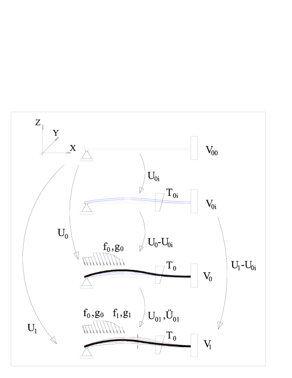
2 Configurations of a structure
-
1.
is the geometric reference configuration, where the displacements are assumed to vanish. For a beam, is the straight configuration. Let be the reference position of a material point.
-
2.
is the initial configuration of the body, where the temperature field is constant and where no external force is applied. This configuration is relevant in the case of geometric imperfections, where differs from . In this paper, however, we assume , i.e. . The stress may not vanish since a self-equilibrated stress may exist.
-
3.
is the equilibrium configuration under static external loads , and a temperature field resulting in a displacement , a relative displacement between and equal to and a stress field .
-
4.
is the instantaneous configuration of a vibrating structure subjected to the static loads , , to the temperature field and to dynamic volume and surface forces and . The relative displacement field between and is indicated by . In practical situations , and may vary with time, e.g. on a daily period, but their variations are supposed to be very slow with respect to free vibrations of the structure. This decomposition of a given external force into a static part and dynamic part is convenient but not unique, e.g. it may depend on the time interval considered if two different static loads are successively imposed. Therefore, the total response of the structure does not split uniquely in a static component and a dynamic response.
3 Constitutive law and physical linearization
Based the objectivity principle, (see e.g. Mandel, (1966, p. 602)), the Helmholtz free energy can be defined as a function of the Green-Lagrange strain tensor
| (1) |
and of the temperature , viz. . As usual, indicates the dot product and is the displacement measured with respect to the given reference configuration . When and the temperature variations are small, can be approximated by a truncated series expansion. Truncating at the second order around the given initial configuration , characterized by and (physical linearization) leads to
| (2) |
where denotes the doubly contracted inner product, the fourth order tensor of the elastic constants, the temperature variation and a diagonal second order tensor accounting for thermal expansion, the initial volume entropy and the specific volume heat [ ]. When a St. Venant-Kirchhoff material is considered, one has
| (3) |
where is the outer tensor product; is the second order identity tensor; is the fourth order identity tensor; and are the Lamé coefficients, is the thermal dilation coefficient. As it is well-known, the following identities hold:
| (4) |
where is the Young modulus, is the Poisson ratio. In this case, the Helmholtz energy (2) becomes
| (5) |
Eq. (2) leads to a constitutive law linear with respect to and :
| (6) |
where is the (second) Piola-Kirchhoff symmetric stress tensor, the index means non-dissipative. Eq. (6) also reads
| (7) |
For isotropic materials having elastic non-linear constitutive behaviour, a direct generalization of (7) can be defined. It is called second order elasticity (Mandel,, 1966, p. 607), supplemented here by the self-equilibrated stress :
| (8) |
where and are the material parameters introduced in addition to the usual ones , and .
Remark: the temperature variations can be considered small when
| (9) |
viz. when strains associated with them are small with respect to unity, similarly to strains fulfilling condition . For isotropic materials, the temperature variations are small if . This condition is consistent with the assumption of physical linearization.
4 A Hu-Washizu functional with additional stress constraints
In this section, a special representation of the problem at hand is introduced, in view of taking into account stress constraints in a three-dimensional framework without forgetting about compatibility issues. A Hu-Washizu (H-W) functional depending on the stress the strain measure and the displacement , considered independent is supplemented with constraints on the stress, in order to model thin bodies. Let , and denote spaces of smooth enough displacement fields, of symmetric second order tensor fields and scalar fields of Lagrange multipliers, respectively. The proposed H-W functional reads
| (10) |
with , and , where is the number of stress constraints and is the given displacement on the boundary . Note that is a functional defined on fields. At a solution of the static problem, the functional above satisfies the stationarity with respect to the fields. The last term leads to linear stress constraints:
| (11) |
where is a vector and is a second order constant tensor. Eq. (11) imposed on carries over to an equivalent condition on the Cauchy stress . The use of this kind of constraints to derive beam equations from 3D elasticity is illustrated in Section 7. The case of a general 3D structure with no constraint can be addressed by formally setting and . The well-known impossibility to derive beam or plate equations from purely kinematical assumptions in the three-dimensional equations of elasticity in pure displacement motivate the introduction of internal constraints as in (Nardinocchi and P. Podio Guidugli,, 1994), (Lembo and Podio Guidugli,, 2001). These constraints enable one to use a pure displacement approach while mimicking the averaging process underlying the convergence of the equations of elasticity when the aspect ratio tends to zero. The derivation of lower-dimensional models without assumptions can rely on -convergence (Acerbi Buttazzo,, 1986), asymptotic analysis (Ciarlet,, 1980), or energy methods (Babuska et al.,, 1992). This paper aims at deriving the equations governing the evolution of thin structures subject to prestress states without above mathematical apparatus.
4.1 Action functional and stationarity conditions
While the stationarity of the H-W functional leads to statics, the action functional leads to elastodynamics over a time interval . Let us set . The kinetic energy , combined with the H-W functional enables one to define the action
| (12) |
Hamilton’s principle is given by , where small variations are considered. The stationarity operator is intended as isochronous, viz. and (see also Quadrelli and Atluri, (1999)). Hamilton’s principle leads to the stationarity conditions
| (13) |
In the physically linear case, Eq. (13-3) corresponds to (6). If isotropy is assumed, Eq. (13-3) is equal to (7). The first equation expresses the stress constraints, the second one defines the strain , which differs from due to the stress constraints. Moreover, depends on the strain accounting for the Lagrange multipliers and not on the standard strain measure . The stationarity condition of the action with respect to displacements leads to
| (14) |
where it has been used the identity on , given in (13). Moreover, the virtual strain is defined by
| (15) |
Integrating by parts in time leads to the virtual works principle at every
| (16) |
where
| (17) |
denote the virtual work of internal, inertia and external forces, respectively. Finally, by integration by parts, one obtains the corresponding strong form equation and the boundary conditions on :
| (18) |
with the initial conditions and in .
5 Physical linearization, strain-rotation domains and dominant terms in the strain energy
Let and denote the fields defining the equilibrium at time . The strain energy density associated with the strain field reads
| (19) |
where is given by (5). The displacement gradient writes
| (20) |
where the symmetric tensor is called small strain tensor, while the skew-symmetric part is called the small rotation tensor. For brevity, hereinafter they will be referred to as strain tensor and rotation tensor. In the same way, the strain increment (15) writes
| (21) |
5.1 A global measure for strains and for rotations and a hierarchy for the strain energy terms
In view of finding out the dominant terms in (19), let us introduce the solution-dependent scalar parameters and as follows:
| (22) |
where is the -norm associated with the domain . The strain measure is supposed to be small. Observe that: (i) is only defined whenever . Thus infinitesimal rigid body motions at initial temperature are excluded from the following analysis; (ii) If the rotations are not large, is a rotation tensor and the quantity is a global measure of the rotations. Hence, can be interpreted as a global index of the relative amplitude of rotations with respect to strains. As a result (see Eq. (1))
| (23) |
Under dynamic conditions and provided that the vibration frequency is bounded, one also has and . In addition, let us make a consistent hypothesis on the self-equilibrated prestress :
| (24) |
Since the Lagrange multipliers fulfill the relationship for all
| (25) |
then, provided the stress constraints are linearly independent, , is the solution of a linear Gram system and splits as follows (see Appendix):
| (26) |
where , and can be evaluated analytically in simple cases. This implies that the Lagrange multipliers, (Eq. (13-2)) and split in terms of the same order.
From Eqs. (13) and (26), the stress splits in four terms:
| (27) |
where
| (28) |
Finally, assume that
| (29) |
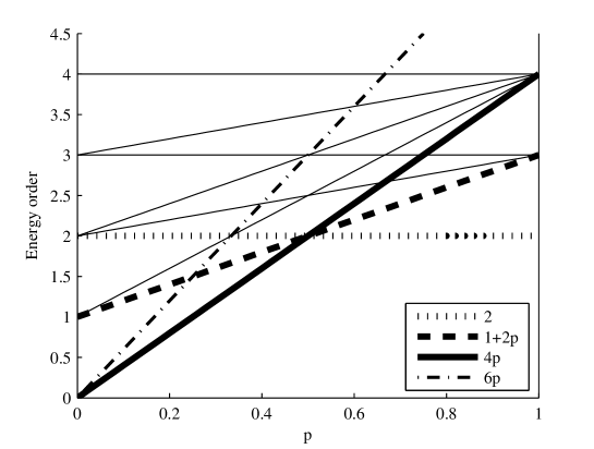
Since , the terms with the smallest exponent are the largest ones. The comparison between different terms must be done for a given -value. If , viz. when is of the same order of magnitude as, or smaller than, (case of small rotations), all non-linear terms in the Green-Lagrange strain and in the Lagrange multipliers can be discarded and the standard condition of small transformation is retrieved. The exponent is introduced in order to account for the possibility of having rotations larger than strains. The complete expression of the strain energy reads (recall Eq. (2), where the terms that depends only on the temperature are omitted for brevity):
i.e. , where
More precisely,
| (30) |
Eq. (30) shows all terms of the strain energy not depending on . The exponents of these energy terms are indicated in Figure 2 and in Table 2. The strain and rotation measures and lead to a hierarchy between the different terms. For every value, the smallest exponents are , (see Fig. 2). Then, the dominant terms are
| (31) |
Likewise, the dominant contribution to splits in three terms:
In summary, one can write
| (32) |
with
A strain energy containing only the three dominant terms, viz. , can be directly derived starting from the Hu-Washizu functional (10), provided that the strain measure is chosen as follows:
| (33) |
The virtual works of the internal forces (see (17), (21) and (28)) read
| (34) |
where .
5.2 Definition of ”strain-rotation domains” and of approximated expressions of the strain energy
Eq. (32) reveals the dominant energy terms. However, it is also interesting to find the strain-rotation domains (depending on and ) where the approximation of the exact strain energy by a simplified expression is acceptable. Three domains are of special interest:
- (a)
-
The domain where
(35) Eq. (35) represents the situation usually called of small perturbations. The corresponding virtual work of internal forces reduces to ; see Eq. (34). As it is seen hereafter, a suitable name for is domain of small strains and relatively small squared rotations (the ratio is small).
- (b)
-
The domain where
(36) i.e. three energy terms are considered together, of order , and , after the discussion of the previous Section. The virtual work reduces to
This region is the domain of small strains and relatively moderate squared rotations (the ratio ), called moderate rotation domain for brevity.
- (c)
-
The domain where
(37) and i.e. the energy term of order is larger than all the others (domain of small strains and relatively large squared rotations, i.e. the ratio is large).
In order to draw these domains, let us introduce a small positive number , for instance . Then, the situations and can be distinguished, since for the dominant term is of order and in the other case the term of order is the largest (Figure 2). When , look for the conditions on and such that all energy terms are small compared with the second order term. The following system of inequalities defines :
| (38) |
Every condition enjoys a simple log-log representation, , since , where and are integer numbers. For instance, when , one has , which relates with . This condition is associated with a line which is the bottom limit of the domain ; see Figure 3a. If , one has , leading to the condition , associated with an horizontal line as shown in same Figure. This means that the ratio between the energy term of order 3 and that of order 2 is smaller or equal to , provided that . Still assuming , one can define the conditions such that all the energy terms are small compared with that of order , except those of order and :
| (39) |
The third relationship shows that inside this domain, the ratio between the term of order and that of order may be either small, equal or greater than . When , the conditions such that all the energy terms are small compared with that of order read:
| (40) |
This set is associated with the approximated energy (37). If the terms of order and are not small, one has
| (41) |
The set is associated to the approximated energy (36). Inside this domain, three energy terms (of order , and ) are retained. The ratios and and their inverses (Eqs. (39), (41)) give an estimation of the relative amplitude of these dominant terms.
Observe that is extended to large rotations ( close to ) because we have compared the energy terms of the first four rows of Table 2 characterizing the physically linear and isotropic constitutive law (7). However, it is of interest here to determine the conditions under which the physical linearization is a reasonable approximation of any real material behaviour. It is expected that this is the case when the rotations are not too large. In order to derive sharp bounds on the rotations, the quadratic constitutive law (8) has to be considered, and the associated strain energy must be computed. This leads to (see also (27))
| (42) |
i.e. some energy terms have to be added to those of the physically linear case, as indicated in Table 2. Then, the same conditions as in (38)-(41) are considered, with substituted by , in order to compute the conditions under which all the physically non-linear terms are small compared with the dominant ones, either of order 2 or 4p. These conditions define the regions depicted in Figure 3b: they are the strain-rotation domains where the physical linearization is admissible. An important difference with respect to Figure 3a is that and are bounded by the vertical line , equivalent to , viz. the squared rotations, not only the strains, must be small. It can be proven that this limitation derives from the condition , imposing that the term of order associated with the physically non-linear law remains small compared with the term of order , dominant for .
The condition of having small Green-Lagrange strain reads: . It easy to identify in Figure 3 the domains in the strain-rotation plane where the first, the second and the fourth term of are less or equal to . It can be also proven that the condition of having a small third term, i.e. , is fulfilled in the three sets , and .
Other approximations retaining at least four energy terms are possible. However, (a), (b) and (c) define situations often discussed in the literature and for this reason the present analysis is restricted to them. Case (b), collecting three terms, is formally more complex than the others and is discussed in detail hereinafter.
5.3 Numerical example: ”exact” values of and and comparison of the exact and ”simplified” energy maps
Consider a problem of plain stress elasticity (, the dimension of the problem, is equal to ). The corresponding conditions on the Piola-Kirchhoff tensor are . A St.Venant- Kirchhoff material is chosen with and . Then
| (43) |
where due to plain stress assumption and
| (44) |
is the 2D Green-Lagrange strain with The relevant H-W functional is given by (10), without the term depending on and with given by (43-1). For a static problem with the external volume force and surface force , the weak form of the equilibrium equation reads:
| (45) |
with and defined by the right-hand side of Eq. (15). Eq. (45) is a non-linear partial differential equation, which can be discretized by a standard finite element method. The standard Newton algorithm has been implemented in the code FreeFEM++ (Danaila et al.,, 2003): given the displacement at iteration , the increment is computed by
with
Set . Repeat until is small enough.
The structure examined in this example is a parallelepiped beam lying in the -plane, the dimensions are and . The beam is clamped at both ends and the volume load is . Exploiting the symmetry of the problem, only a half-beam is meshed, with the boundary conditions for and and for and . The material parameters (steel) read . A mesh of triangular elements has been chosen, with two elements inside every cell of a regular grid of 15x375 squares. The finite element space is of P1 type. The numerical simulations give the results collected in Tables 3 and 4, where , , , and
| (46) |
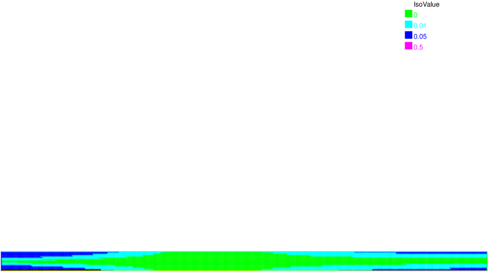
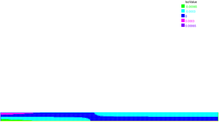
The last column of Table 4 provides a global estimation of the energy error between the exact and the approximated energies and . Observe the maximum absolute value of the strain , reported in the third column of Table 3: in the first four cases it is less than which is the limit elastic strain for a steel having yielding stress approximately equal to . For these situations, the material is truly physically linear. Conversely, when , see the last row of Table 3, the maximum absolute value of is larger than . Hence, the physical linearity is truly fulfilled only for steels having a greater yielding stress. The coordinates of the strain-rotation points associated with each value are reported in the seventh and eighth columns of Table 3. The corresponding graphical representation is given in Figure 3-b, depicted assuming . The map , viz. the strain energy density at the static equilibrium is shown in Figure 4. The energy density corresponding to the approximated strain energy is given in Figure 5. The relative difference of energy density between the two cases is illustrated in Figure 6. With a surface load and , the results are similar, as one can see from Tables 5, 6 and Figure 7. This confirms that and are not too sensitive to the load distribution.
6 Dissipative stress, Hu-Washizu functional and damping pseudo-potential with stress constraints
The linear law (6) can be generalized by adding to a dissipative term:
| (47) |
The index indicates the dissipative part of the stress. Let
| (48) |
be the functional associated with a dissipative stress. It is assumed that it depends on the dissipative stress , the generic strain flow and , i.e. the Lagrange multipliers associated with the constraints imposed on . Moreover, the actual strain flow plays the role of additional parameter: for this reason it is separated from the main variables by the semi-colon ”;”, instead of the comma. The actual strain flow is computed from the problem associated with the Hu-Washizu functional defined in Eq. (54). The scalar non-negative and convex function is called pseudo-potential or dissipation potential. A classical definition is , i.e. a quadratic function. For an isotropic material, one has , where and are analogous to the Lamé constants and . The stationarity conditions imposed on (48) lead to following strong form expressions
| (49) |
The first equation indicates the stress constraints imposed on , the second one shows that the strain flow governing the dissipative behaviour is not equal to the time derivative of the strain when . Finally, the third equation is the constitutive law for the dissipative stress, obtained from the pseudo-potential . The constraints on the dissipative stress read
| (50) |
where are known from the analysis of the non-dissipative part of the stress. Following the procedure indicated in the Appendix, one can prove that , is the solution of a linear Gram system. Therefore
| (51) |
Using Eqs. (49) and (51), one obtains
| (52) |
where the following four terms of different orders are distinguished:
| (53) |
In order to define the non-dissipative part of the stress, as well as the equilibrium equation, the following Hu-Washizu type functional is introduced:
| (54) |
Eq. (54) should be compared with (10). An attentive reader can see that the functional depends on the non-dissipative part of the stress instead of on the total stress . Moreover, an additional dependence on is introduced, where is the stationary solution of (48). Stationarity imposed on leads to the strong form expressions:
| (55) |
Moreover, recalling (12) and imposing stationarity in the displacements, one obtains the following weak form equilibrium equation:
where is defined in (17), is also given in (17), with and
| (56) |
The virtual work of inertia forces is the same as in the previous non-dissipative case. The dynamics of the system is ruled by (18), where is given by (47). The case of moderate rotations is obtained by just substituting with in Eqs. (48) and (54). This corresponds to the substitutions and , where (see Eq. (34))
| (57) |
7 Accounting for a static prestress
As already discussed, when a static prestress due external mechanical and/or thermal loading occurs, the structure passes from the state to a state . It is interesting to write the equations governing the equilibrium at the generic configuration as a function of the unknown displacement , expressing the motion with respect to , as illustrated in Figure 1. This can be easily done subtracting the equilibrium equations established in the previous sections, written at and at . Both equilibrium conditions at and should be written, together with the other expressions coming from the stationarity of the relevant H-W type functional. For the sake of simplicity, only the weak form of the dynamic equilibrium is reported in the analysis of this section. As seen above, the virtual work of the internal forces is indicated by in the general case, and by in the case of moderate rotations. All the equations of this section are written as function of , and then refer to the general case. However, the formal substitution of at the place of gives the equations for the moderate rotation case.
The static problem defining the prestressed configuration reads
| (58) |
where are the Lagrange multipliers associated with the static problem and the prestress accounts for the temperature field . The dynamic problem defining the generic configuration reads
| (59) |
where are the Lagrange multipliers computed for the dynamic problem. The difference between (59) and (58) leads to
| (60) |
with
| (61) |
knowing that . Eq. (60) describes the dynamics around a statically prestressed configuration for the general case. Observe that all the equations are defined in the Lagrangian configuration , free of any external prestress effect by definition. The case of moderate rotations is retrieved introducing in the same equation instead of and instead of . From Eq. (31) and recalling (36), (52) and (53), Eq. (61) becomes
| (62) |
8 Moderate rotations and Bernoulli-Navier kinematic assumptions: undamped case
In this section, the stationarity conditions (13) with suited stress constraints are used in conjunction with the strain measure (33) for moderate rotations and the so-called Navier kinematic assumptions for beams, in order to obtain the corresponding strong form of the dynamic equilibrium equations. This analysis will enable a better understanding of the general equations previously presented. In particular, a simple way of estimating and is suggested with reference to the example of a clamped-clamped beam. In the non deformed configuration , the beam axis coincides with the cartesian axis and the beam motion is supposed to be limited to the plane . A quadratic Helmholtz energy is adopted, leading to a linear constitutive law depending on the tensors and :
| (63) |
with
| (64) |
For an isotropic material, one has . Moreover, since , one has . The Navier kinematic assumption reads
| (65) |
where are the X-and Y-displacement fields; the apex ′ indicates the derivation with respect to . The strains and read:
For the prestress , we assume:
Off-diagonal terms of may not vanish. Nonetheless, they have no influence on the following analysis, since they are associated with zero virtual strain components in the virtual work product. The thermal and load fields write
The stress constraints usually imposed to retrieve beam equations are , formally expressed by the conditions
| (66) |
Eqs. (22),(24) and (29) written for this case become
| (67) |
where is the area of the generic beam section; is the inertia moment and is the beam length. Then, the same procedure as in the general case can be applied here, in order to determine the strain-rotation domains , and . As it is well-known, the Navier-Bernoulli kinematic assumptions entails that all shear strains, i.e. the off-diagonal elements of , are equal to zero. As a result, one can easily prove that also the terms of order , and in the strain energy
| (68) |
become zero (see Figure 8 and compare to Figure 2). As a result, the strain-rotation domains are not the same as in the general case, as illustrated in Figure 9. The difference is highlighted by the small region excluded in the general case and admitted by the Navier kinematic conditions. Inside this region, the pertinence of the Navier assumptions (65) should be further investigated. Other kinematic assumptions, like for instance those of Timoshenko, appear to be more sound.
8.1 Strong form equations
Eqs. (63), (66) and (65) lead to the Lagrange multipliers
| (69) |
from which (see (64)) and
where and while the other stress components are zero. Moreover, the virtual works read
| (70) |
where and are the reaction forces and the reaction moment at the boundary . Observe the second and third term in : it can be proven that the ratio between the third term (rotational inertia) and the second term (translational inertia) reads , where is the beam width. When the squared aspect ratio is small, is small too. Note that this ratio can be easily expressed in terms of and when and . In this case, Eqs. (67-1,2) entail . Hence, under these assumptions and suffice to have small. The first condition is always fulfilled due to physical linearization assumption, while the second one is equivalent to and (see Figure 9) and is satisfied in a large portion of . For simplicity, the rotational inertia is always omitted hereinafter. The strong form equations corresponding to (70) are derived using the standard procedure:
| (71) |
where and are the horizontal and vertical loading per unit beam length, respectively; is a couple per unit length. The boundary conditions of type involving the external forces , and the external couple at the ends of the beam, are not reported for brevity. At the configuration , one has , with zero loads, entailing and . This implies that is constant along the length of the beam. Since zero force is applied on , i.e. , this constant is equal to zero and the same holds for . This means that the initial self-equilibrated stress is zero and the equilibrium equations become
| (72) |
This is the general expression of the beam equation with temperature field. The corresponding expression of the strain energy (see (31) and (36)) becomes
| (73) |
8.2 The geometric interpretation of and
In this Section, an interpretation of and in terms of suitable deflection and shape ratios, and as functions of the temperature field is provided for the case of a homogeneous beam. A first example concerns a beam with very small bending stiffness, i.e. . A static vertical load is applied at the midspan, where it induces a transversal displacement . Moreover, and an axial temperature field is introduced. Then, Eq. (72) becomes
| (74) |
where is the constant horizontal reaction at . Boundary conditions write , , and . Since is piecewise constant, with a discontinuity at the midspan, integration of the first equation in (74) yields
where is the averaged temperature variation. It follows i.e. when the axial temperature field is constant, even if non-zero. In this case and by using (67), one obtains
| (75) |
which provide a simple interpretation of and in terms of temperature difference and of ratios between the maximum displacements and the beam length. Hence, the strain-rotation domains of Figure 9, which depend on and , can also be interpreted using these ratios. For instance, consider the case of zero temperature field and given value, such that : the strain-rotation points corresponding to this situation and for different values of are depicted in Figure 9-b: they have the same -value (constant ) and different -values. The larger , the larger : then, according to the value of , the point representing the structural state may belong to any of the sets or and the relevant equilibrium equation is different in each case. Since the strain-rotation domains depend on , Figure 9 refers to the case . Observe in addition that gives an estimate of the relative importance of the thermal and mechanical strains.
Let us now consider a homogeneous beam with a distributed vertical static load , a generic temperature field and with . The same structure has been studied in the numerical examples of Section 5.3. Eq. (72) becomes
| (76) |
For the -direction, the boundary conditions (b.c.) are and in the vertical direction one has . Integrating the first equation with the b.c. at and leads to
| (77) |
It follows, according to (76-1)
| (78) |
where has the same definition as in the previous example. Assume that and are constant and substitute (78) into the definition (67) of . Hence
In order to have a better understanding of the geometrical meaning of , the solution , depending on , and should be analytically expressed. However, this is not a simple task in general. Hence, accounting for the b.c., we assume here that the deformed shape is approximately co-sinusoidal:
| (79) |
Hence, by using the definitions (67), one obtains
| (80) |
where , with the beam width. When the transversal displacement is different from zero, the ratio between the thermal and mechanical contributions in is equal to
| (81) |
The interest of Eq. (80) is that it gives a geometrical interpretation for the case of beams of the quantities and defined in (22) for the general case and in (67) when the Navier-Bernoulli kinematic assumptions are adopted. They can be easily related to geometrical ratios involving the maximum deflection, the width and the length of the beam. These geometrical ratios are known to be important for beam analysis, but they are clearly related here to the tensorial quantities of a full 3D formulation of the structural problem. When both maximum deflection and geometry of the beam are known (or estimated), it is easy to find the corresponding point in strain-rotation domains and to establish how many terms need to be taken into account for the computation of the solution.
In order to find the explicit expression of the strain energy, note that constant entails from Eq. (78)
| (82) |
and . Hence, using (79) and the expression of given in (80), the strain energy contributions (73) read
The ratio between the energy terms of order and reads
and it only depends on the ratio . The virtual works of internal and external forces (see (70)) read
with supposed constant, and by the virtual work principle, one obtains
| (83) |
which provides a simple nonlinear relationship between and . Eq. (83) does not depend on since this quantity is assumed constant on the beam length. Using Eq. (83) with and supposing , and like in Section 5.3, one obtains the values collected in the first column of Table 7. Moreover, by means of (80), it is easy to compute and . These values are good estimations of the corresponding quantities computed from the numerical tests (Table 3). The difference between estimated as in (80) and in the numerical analysis is due to the shear stress as well as the component. On the other hand, issued by the numerical analysis and the analytical estimation of according to (80) are very close. The corresponding co-ordinates in the strain-rotation domain are reported in the fifth and the sixth column of Table 7 (see also Figure 9). The influence of a thermal field with , and on the strain can be estimated as follows: Eq. (83) with the true temperature field is used to compute , then and are separately evaluated, as well as their ratio (see the seventh column of Table 8). A more useful comparison may be done by the ratio between of this last case and for the case at the same level of (see the last column of Table 8). This ratio correctly neglects the influence of .
8.3 Equilibrium around a prestressed configuration: strong form equations
By subtracting Eq. (72) written at the state from the same equation at the state , one obtains
| (84) |
where , are the axial and transversal displacements characterizing the statically prestressed configuration, measured between and ; is the axial temperature field; is the static axial prestress; the unknowns , are the displacements between the dynamic configuration and the static one. The first and the second term of the bending equation (84-2) are linear. The second one is related to the static configuration (, and ): it is the effect of the static prestress due to external static loads, i.e. it is not self-equilibrated and is associated with a body configuration different from . The bending equation in (84) contains a term coupling with the static and the dynamic rotations and . This term seems to be of paramount importance since experimental investigations (Treyssède,, 2006) prove that pre-bending effect play a crucial role, and not only prestress. When is different from zero, this term cannot be neglected in front of the static prestress contribution associated with . This situation occurs when a pulsating axial loading is applied at one end of the beam, inducing parametric resonance. In this case, the first equation in (84) becomes
where by assumption. The influence of the axial inertia on the solution is discussed, e.g., by Ribeiro, (2001).
9 Moderate rotations and Bernoulli-Navier kinematic assumptions: viscous damping case
The stress when linear viscous damping occurs is given by (see (47), (49) and (55)):
where the Lagrange multipliers can be computed imposing the constraints and , where and are given in (66). Since the two parts of the stress must be separately equal to zero, the Lagrange multipliers do not change with respect to the non-dissipative case, and they are given in Eq. (69). Hence, their time derivatives can be computed under the assumption, previously discussed, that the time variations of the temperature field are very small compared to those of displacements. Hence, and , with . As a result, one has
Let us assume that damping is proportional to the stiffness and to the mass, viz. with and . Then, the constraints on the dissipative stress read
It entails , and with
This expression relates the ”structural” viscous damping coefficient and the ”material” parameters , and . The virtual work of dissipative forces becomes (see Eq. (56))
and the strong form equations read
| (85) |
When , i.e. damping proportional to the stiffness, one has and . Moreover, around a static configuration with prestress , one has
| (86) |
10 Conclusions
Based on a Hu-Washizu functional accounting for stress constraints, an original derivation of the dynamic equations for thin prestressed and prestrained structures from continuum mechanics has been presented. The assumption of small strains and moderate rotations, as well as the physical linearization, have been formalized by the notion of strain-rotation domains associated with new strain and rotation global measures. The corresponding approximated expressions for the strain energy have been justified by 2D non-linear finite element investigations. The presence of a generic mechanical or thermal prestress and physically linear viscous damping has been discussed in detail. In particular, damping is introduced by the original definition of a pseudo-potential with stress constraints. Coupled beam equations governing traction and bending for small strains and moderate rotations have been derived by using the proposed general procedure.
References
- Acerbi Buttazzo, (1986) Acerbi, E., Buttazzo, G., 1986. Limit problems for plates surrounded by soft material, Arch. Rational Mech. Anal. 92, 355-370.
- Adhikari Woodhouse, (2001) Adhikari S., Woodhouse J., Identification of Damping: Part 1, Viscous damping; Part 2, Non-viscous damping, J. Sound Vibr. 243(1), 43-88.
- Amabili, (2005) Amabili, M., 2005. Theory and experiments for large-amplitude vibrations of rectangular plates with geometric imperfections, J. Sound Vibr. (in press).
- Argoul and Le, (2003) Argoul, P., Le, T.P., 2003. Instantaneous indicators of structural behaviour based on continuous Cauchy wavelet transform, Mech. Syst. Signal Proc. 17, 243-250.
- Babuska et al., (1992) Babuska, I., Szabo, B. A. and Actis, R. L., 1992. Hierarchic Models for Laminated Composites, Int. J. Num. Meth. Engrg. 33, 503-535.
- Basseville et al., (2004) Basseville, M., Mevel, L., Goursat, M., 2004. Statistical model-based damage detection and localization: subspace-based residuals and damage-to-noise sensitivity ratios, J. Sound Vibr. 275, 769-794.
- Basseville et al., (2006) Basseville, M., Bourquin, F., Mevel, L., Nasser, H., Treyssède, F., 2006. Handling the temperature effect in SHM: combining a subspace-based statistical test and a temperature-adjusted null space, in: Proc. 3rd European Workshop on Structural Health Monitoring, Granada, Spain.
- Ciarlet, (1980) Ciarlet, P.G., 1980. A justification of the von Kármán equations, Arch. Rational Mech. Anal. 73, 349-389. Ciarlet and Gratie, 2001]PGCgeneralvonkarman Ciarlet, P.G., Gratie, L., 2001. Generalized von Kármán equations. Journal de Math ématiques Pures et Appliquées 80(3), 263-279.
- Danaila et al., (2003) Danaila, I., Hecht, F., Pironneau, O., 2003. Simulation numérique en C++, http://www.freefem.org/.
- Farrar et al., (1994) Farrar, C.R., Baker, W.E., Bell, T.M., Cone, K.M., Darling, T.W., Duffey, T.A., Eklund, A., Migliori, A., 1994. Dynamc characterization and damage detection in the I-40 bridge over the Rio Grande. Technical Report, LA-12767-MS, Los Alamos National Laboratory, NM (USA).
- Géradin and Rixen, (1995) Géradin, M., Rixen, D., 1994. Mechanical vibrations: theory and applications to structural dynamics. Wiley.
- Kerschen et al., (2003) Kerschen, G., Lenaerts, V., Golinval, J.-C., 2003. Identification of a continuous structure with a geometrical non-linearity. Part I: Conditioned reverse path method., J. Sound Vibr. 164(4), 889-906.
- Lembo and Podio Guidugli, (2001) Lembo, M., Podio Guidugli, P., 2001. Internal constraints, reactive stresses, and the Timoshenko beam theory, J. Elasticity 65, 131-148.
- Mandel, (1966) Mandel, J., 1966. Cours de mécanique des milieux continus, Tome 2. Gauthier-Villars, Paris.
- Nardinocchi and P. Podio Guidugli, (1994) Nardinocchi, P., Podio Guidugli, P., 1994. The equations of Reissner-Mindlin plates obtained by the method of internal constraints, Meccanica 29, 143-157.
- Nasser, (2006) Nasser, H., 2006. Surveillance Vibratoire de Structures Mécaniques sous Contraintes Thermiques, PhD thesis, Université de Rennes I, France (in French).
- Peeters and De Roeck, (2001) Peeters, B., De Roeck, G., 2001. One-year monitoring of Z-24 bridge : environmental effects versus damage events. Earthquake Engineering and Structural Dynamics, 30(2), 149-171.
- Perignon et al., (2003) Perignon, F., Bellizzi, S., Cochelin, B., 2003. Application de l’équilibre harmonique au calcul de la réponse forcée de structures minces en non-linéaire géométrique, in: Publications du LMA, N. 156, Marseille, France, pp. 59-78
- Quadrelli and Atluri, (1999) Quadrelli, M.B., Atluri, S.N., 1999. Mixed variational principles in space and time for elastodynamics analysis, Acta Mech. 136, 193-208.
- Ribeiro, (2001) Ribeiro, P., 2001. The second harmonic and the validity of Duffing’s equations for vibration of beams with large displacements, Comp. Struct. 79, 107-117.
- Rosenberg, (1962) Rosenberg, R.M., 1962. The normal modes of nonlinear n-degree-of-freedom system, J. Appl. Mech. 29, 7-14.
- Sohn et al., (2003) Sohn, H., Worden, K., Farrar, C.R., 2003. Statistical damage classification under changing environmental and operational conditions. J. Intell. Mat. Syst. Struct. 13(9), 561-574.
- Treyssède, (2006) Treyssède, F., 2006. Numerical and experimental study of the vibrational modes of thermally prestressed and prebent beams, in: Proc. 13th International Congress on Sound and Vibration, Austria.
- Vakakis, (1997) Vakakis, A.F., 1997. Non-linear normal modes (NNMs) and their applications in vibration theory: an overview. Mech. Syst. Sig. Proc. 11, 3-22.
- Wenzel and Pichler, (2005) Wenzel, H., Pichler, D., 2005. Ambient Vibration Monitoring. E-Book, ISBN; 0-470-02431-3.
11 Appendix: Lagrange multipliers
In this Section, we show how to compute the Lagrange multipliers. The stress constraints write
| (87) |
with . Eq. (87) is equivalent to
or where , , and
By virtue of the symmetry and positivity of it is easy to prove that is symmetric positive definite and therefore invertible, provided that tensors are linearly independent. Hence, the Lagrange multipliers read . Then, the assumptions (22), (23) and (24) prove that In particular, the constraints (66) leads to
and
For the dissipative stress, one has analogous constraints
Then where and
is symmetric positive definite. For a beam
and