Multicasting Correlated Multiple Sources to Multiple Sinks over a Noisy Network

Abstract:  The problem of network coding for multicasting a single source to multiple sinks has first been studied by Ahlswede, Cai, Li and Yeung in 2000, in which they have established the celebrated max-flow mini-cut theorem on non-physical information flow over a network of independent channels. On the other hand, in 1980, Han has studied the case with correlated multiple sources and a single sink from the viewpoint of polymatroidal functions in which a necessary and sufficient condition has been demonstrated for reliable transmission over the network. This paper presents an attempt to unify both cases, which leads to establish a necessary and sufficient condition for reliable transmission over a network for multicasting correlated multiple sources to multiple sinks. Here, the problem of separation of source coding and network coding is also discussed.

Index terms:  network coding, multiple sources, multiple sinks, correlated sources, entropy rate, capacity function, polymatroid, co-polymatroid, mini-cut, transmissibility

1 Introduction

The problem of network coding for multicasting a single source to multiple sinks has first been studied by Ahlswede, Cai, Li and Yeung [1] in 2000, in which they have established the celebrated max-flow mini-cut theorem on non-physical information flow over a network of independent channels. On the other hand, in 1980, Han [3] had studied the case with correlated multiple sources and a single sink from the viewpoint of polymatroidal functions in which a necessary and sufficient condition has been demonstrated for reliable transmission over a network.

This paper presents an attempt to unify both cases and to generalize it to quite a general case with stationary ergodic correlated sources and noisy channels (with arbitrary nonnegative real values of capacity that are not necessarily integers) satisfying the strong converse property (cf. Verdú and Han [6], Han [4]), which leads to establish a necessary and sufficient condition for reliable transmission over a noisy network for multicasting correlated multiple sources altogether to every multiple sinks.

It should be noted here that in such a situation with correlated multiple sources, the central issue turns out to be how to construct the matching condition between source and channel (i.e., joint source-channel coding), instead of of the traditional concept of capacity region (i.e., channel coding), although in the special case with non-correlated independent multiple sources the problem reduces again to how to describe the capacity region.

Several network models with correlated multiple sources have been studied by some people, e.g., by Barros and Servetto [9], Ho, Médard, Effros and Koetter [13], Ho, Médard, Koetter, Karger, Effros, Shi and Leong [14], Ramamoorthy, Jain, Chou and Effros [15]. Among others, [13], [14] and [15] consider (without attention to the converse part) a very restrictive case of error-free network coding for two stationary memoryless correlated sources with a single sink to study the error exponent problem, where we notice that all the arguments in [13], [14] and [15] can be validated only within the narrow class of stationary memoryless sources of integer bit rates and error-free channels (i.e., the identity mappings) all with one bit (or integer bits) capacity (these restrictions are needed solely to invoke “Menger’s theorem” in graph theory). The main result in the present paper is quite free from such severe restrictions, because we can dispense with the use of Menger’s theorem.

On the other hand, [9] revisits the same model as in Han [3], while [15] focuses on the network with two correlated sources and two sinks to discuss the separation problem of distributed source coding (based on Slepian-Wolf theorem) and network coding. It should be noted that, in the case of networks with correlated multiple sources, such a separation problem is another central issue, although it is yet far from fully solved. In this paper, we mention a sufficient condition for separability in the case with multiple sources and multiple sinks. (cf. Remark 5.2).

On the other hand, we may consider another network model with independent multiple sources but with multiple sinks each of which is required to reliably reproduce a prescribed subset of the multiple sources that depends on each sink. However, the problem with this general model looks quite hard, although, e.g., Yan, Yeung and Zhang [11] and Song, Yeung and Cai [12] have demonstrated the entropy characterizations of the capacity region, which still contain limiting operations and are not computable. Incidentally, Yan, Yang and Zhang [22] have considered, as a computable special case, degree-2 three-layer networks with $K$-pairs transmission requirements to derive the explicit capacity region. In this paper, for the same reason, we focus on the case in which all the correlated multiple sources is to be multicast to all the multiple sinks and derive a simple necessary and sufficient matching condition in terms of conditional entropy rates and capacity functions. This case can be regarded as the network counterpart of the non-network compound Slepian-Wolf system [21].

We notice here the following; although throughout in the paper we are encountered with the subtleties coming from the general channel and source characteristics assumed, the main logical stream remains essentially unchanged if we consider simpler models, e.g., such as stationary correlated Markov sources together with stationary memoryless noisy channels. This means that considering only simple cases does not help so much at both of the conceptual and notational levels of the arguments. For this reason, we preferred here the compact general settings.

The present paper consists of five sections. In Section 2 notations and preliminaries are described, and in Section 3 we state the main result as well as its proof. In Section 4 two examples are shown. Section 5 provides another type of necessary and sufficient condition for transmissibility. Finally, some detailed comments on the previous papers are given.

2 Preliminaries and Notations

A. Communication networks

Let us consider an acyclic directed graph $G=(V,E)$ where $V=\{1,2,\cdots,|V|\}$ $(|V|<+\infty)$, $E\subset V\times V,$ but $(i,i)\not\in E$ for all $i\in V$. Here, elements of $V$ are called nodes, and elements $(i,j)$ of $E$ are called edges or channels from $i$ to $j$. Each edge $(i,j)$ is assigned the capacity $c_{ij}\geq 0$, which specifies the maximum amount of information flow passing through the channel $(i,j)$. If we want to emphasize the graph thus capacitated, we write it as $G=(V,E,C)$ where $C=(c_{ij})_{(i,j)\in E}$. A graph $G=(V,E,C)$ is sometimes called a (communication) network, and indicated also by ${\cal N}=(V,E,C)$. We consider two fixed subsets $\Phi,\Psi$ of $V$ such that $\Phi\cap\Psi=\emptyset$ (the empty set) with

$$\Phi=\{s_{1},s_{2},\cdots,s_{p}\},$$

$$\Psi=\{t_{1},t_{2},\cdots,t_{q}\},$$

where elements of $\Phi$ are called source nodes, while elements of $\Psi$ are called sink nodes. Here, to avoid subtle irregularities, we assume that there are no edges $(i,s)$ such that $s\in\Phi.$

Informally, our problem is how to simultaneously transmit the information generated at the source nodes in $\Phi$ altogether to all the sink nodes in $\Psi$. More formally, this problem is described as in the following subsection.

Remark 2.1

In the above we have assumed that $\Phi\cap\Psi=\emptyset$. However, we can reduce the case of $\Phi\cap\Psi\neq\emptyset$ to the case of $\Phi\cap\Psi=\emptyset$ by equivalently modifying the given network. In fact, suppose $\Phi\cap\Psi\neq\emptyset$ and let $k\in\Phi\cap\Psi$ for some $k$. Then, we add a new source node $k^{\prime}$ to $\Phi$, and generate a new edge $(k^{\prime},k)$ with capacity $\infty$, and remove the node $k$ from $\Phi$. Repeat this procedure until we have $\Phi\cap\Psi=\emptyset$. The assumption that there are no edges $(i,s)$ such that $s\in\Phi$ also can be dispensed with by repeating a similar procedure. $\Box$

B. Sources and channels

Each source node $s\in\Phi$ generates a stationary and ergodic source process

$$X_{s}=(X_{s}^{(1)},X_{s}^{(2)},\cdots),$$ (2.1)

where $X_{s}^{(i)}(i=1,2,\cdots)$ takes values in finite source alphabet ${\cal X}_{s}$. Throughout in this paper we consider the case in which the whole joint process $X_{\Phi}\equiv(X_{s})_{s\in\Phi}$ is stationary and ergodic. It is then evident that the joint process $X_{T}\equiv(X_{s})_{s\in T}$ is also stationary and ergodic for any $T$ such that $\emptyset\neq T\subset\Phi$. The component processes $X_{s}\ (s\in\Phi)$ may be correlated. We write $X_{T}$ as

$$X_{T}=(X_{T}^{(1)},X_{T}^{(2)},\cdots)$$ (2.2)

and put

$$X_{T}^{n}=(X_{T}^{(1)},X_{T}^{(2)},\cdots,X_{T}^{(n)}),$$ (2.3)

where $X_{T}^{(i)}\ (i=1,2,\cdots)$ takes values in ${\cal X}_{T}\equiv\prod_{s\in T}{\cal X}_{s}$.

On the other hand, it is assumed that all the channels $(i,j)\in E,$ specified by the transition probabilities $w_{ij}:A_{ij}^{n}\to B_{ij}^{n}$ with finite input alphabet $A_{ij}$ and finite output alphabet $B_{ij}$, are statistically independent and satisfy the strong converse property (see Verdú and Han [6]). It should be noted here that stationaty and memoryless (noisy or noiseless) channels with finite input/output alphabets satisfy, as very special cases, this property (cf. Gallager [7], Han [4]). Barros and Servetto [9] have considered the case of stationary and memoryless sources/channels with finite alphabets. The following lemma plays a crucial role in establishing the relevant converse of the main result:

Lemma 2.1

(Verdú and Han [6]) The channel capacity $c_{ij}$ of a channel $w_{ij}$ satisfying the strong converse property with finite input/output alphabets is given by

$$c_{ij}=\lim_{n\to\infty}\frac{1}{n}\max_{X^{n}}I(X^{n};Y^{n}),$$

where $X^{n},Y^{n}$ are the input and the output of the channel $w_{ij}$, respectively, and $I(X^{n};Y^{n})$ is the mutual information (cf. Cover and Thomas [8]). $\Box$

C. Encoding and decoding

In this section let us state the necessary operation of encoding and decoding for network coding with correlated multiple sources to be multicast to multiple sinks.

With arbitrarily small $\delta>0$ and $\varepsilon>0$, we introduce an $(n,(R_{ij})_{(i,j)\in E},$ $\delta,\varepsilon)$ code as the one as specified by (2.4) $\sim$ (2.9) below, where we use the notation $[1,M]$ to indicate $\{1,2,\cdots,M\}$. How to construct a “good” $(n,(R_{ij})_{(i,j)\in E},$ $\delta,\varepsilon)$ code will be shown in Direct part of the proof of Theorem 3.1.

1) For all $(s,j)\ (s\in\Phi)$, the encoding function is

$$f_{sj}:{\cal X}^{n}_{s}\to[1,2^{n(R_{sj}-\delta)}],$$ (2.4)

where the output of $f_{sj}$ is carried over to the encoder $\varphi_{sj}$ of channel $w_{sj}$, while the decoder $\psi_{sj}$ of $w_{sj}$ outputs an estimate of the output of $f_{sj}$, which is specified by the stochastic composite function:

$$h_{sj}\equiv\psi_{sj}\circ w_{sj}\circ\varphi_{sj}\circ f_{sj}:{\cal X}^{n}_{s}\to[1,2^{n(R_{sj}-\delta)}];$$ (2.5)

2) For all $(i,j)$ $(i\not\in\Phi)$, the encoding function is

$$f_{ij}:\prod_{k:(k,i)\in E}[1,2^{n(R_{ki}-\delta)}]\to[1,2^{n(R_{ij}-\delta)}],$$ (2.6)

where the output of $f_{ij}$ is carried over to the encoder $\varphi_{ij}$ of channel $w_{ij}$, while the decoder $\psi_{ij}$ of $w_{ij}$ outputs an estimate of the output of $f_{ij}$, which is specified by the stochastic composite function:

$$h_{ij}\equiv\psi_{ij}\circ w_{ij}\circ\varphi_{ij}\circ f_{ij}:\prod_{k:(k,i)\in E}[1,2^{n(R_{ki}-\delta)}]\to[1,2^{n(R_{ij}-\delta)}].$$ (2.7)

Here, if $\{k:(k,i)\in E\}$ is empty, we use the convention that $f_{ij}$ is an arbitrary constant function taking a value in $[1,2^{n(R_{ij}-\delta)}]$;

3) For all $t\in\Psi$, the decoding function is

$$g_{t}:\prod_{k:(k,t)\in E}[1,2^{n(R_{kt}-\delta)}]\to{\cal X}^{n}_{\Phi}.$$ (2.8)

4) Error probability

All sink nodes $t\in\Psi$ are required to reproduce a “good” estimate $\hat{X}^{n}_{\Phi,t}$ ($\equiv$ the output of the decoder $g_{t}$) of $X^{n}_{\Phi}$, through the network ${\cal N}=(V,E,C)$, so that the error probability $\Pr\{\hat{X}^{n}_{\Phi,t}\neq X^{n}_{\Phi}\}$ be as small as possible. Formally, for all $t\in\Psi$, the probability $\lambda_{n,t}$ of decoding error committed at sink $t$ is required to satisfy

$$\lambda_{n,t}\equiv\Pr\{\hat{X}^{n}_{\Phi,t}\neq X^{n}_{\Phi}\}\leq\varepsilon$$ (2.9)

for all sufficiently large $n$. Clearly, $\hat{X}^{n}_{\Phi,t}$ are the random variables induced by $X^{n}_{\Phi}$ that were generated at all source nodes $s\in\Phi$.

Remark 2.2

In the above coding process, $f_{ij}$ is applied before $f_{i^{\prime}{j\prime}}$ is if $i<i^{\prime}$, and $f_{ij}$ is applied before $f_{i{j\prime}}$ is if $j<j^{\prime}.$ Such an indexing is possible because we are dealing with acyclic directed graphs. This defines the order in which the encoding functions are applied. Since $i<j$ if $(i,j)\in E$, a node does not encode until all the necessary informations are received on the input channels (see, Ahlswede, Cai, Li and Yeung [1], Yeung [2]). In this sense, the coding procedure with the codes $(n,(R_{ij})_{(i,j)\in E},\delta,\varepsilon)$ defined above is in accordance with the natural ordering on an acyclic graph. This observation will be fully used in the proof of Converse part of Theorem 3.1 in order to establish a Markov chain property. $\Box$

We now need the following definitions.

Definition 2.1 (rate achievability)

If there exists an $(n,(R_{ij})_{(i,j)\in E},$ $\delta,\varepsilon)$ code for any arbitrarily small $\varepsilon>0$ as well as any sufficiently small $\delta>0$, and for all sufficiently large $n$, then we say that the rate $(R_{ij})_{(i,j)\in E}$ is achievable for the network $G=(V,E)$. $\Box$

Definition 2.2 (transmissibility)

If, for any small $\tau>0$, the augmented capacity rate $(R_{ij}=c_{ij}+\tau)_{(i,j)\in E}$ is achievable, then we say that the source $X_{\Phi}$ is transmissible over the network ${\cal N}=(V,E,C),$ where $c_{ij}+\tau$ is called the $\tau$-capacity of channel $(i,j).$ $\Box$

The proof of Theorem 3.1 (both of the converse part and the direct part) are based on these definitions.

D. $\lambda$-Typical sequences

Let ${\bf x}_{\Phi}$ denote the sequence of length $n$ such as

$${\bf x}_{\Phi}=(x_{\Phi}^{(1)}),\cdots,x_{\Phi}^{(n)})\in{\cal X}_{\Phi}^{n}.$$

Similarly, we denote by ${\bf x}_{T}\ (\emptyset\neq T\subset\Phi)$ the sequence such as

$${\bf x}_{T}=(x_{T}^{(1)}),\cdots,x_{T}^{(n)})\in{\cal X}_{T}^{n}.$$

We set

$$p({\bf x}_{T})=\Pr\{X_{T}^{n}={\bf x}_{T}\}$$

and let $H(X_{T})$ be the entropy rate of the process $X_{T}$. With any small $\lambda>0$, we say that ${\bf x}_{\Phi}\in{\cal X}^{n}_{\Phi}$ is a $\lambda$-typical sequence if

$$\left|\frac{1}{n}\log\frac{1}{p({\bf x}_{S})}-H(X_{S})\right|<\lambda\quad(\emptyset\neq\forall S\subset\Phi),$$ (2.10)

where ${\bf x}_{S}$ is the projection of ${\bf x}_{\Phi}$ on the $S$-direction, i.e., ${\bf x}_{\Phi}=({\bf x}_{S},{\bf x}_{\overline{S}})$ ($\overline{S}$ is the complement of $S$ in $\Phi$). We shall denote by $T_{\lambda}(X_{\Phi})$ the set of all $\lambda$-typical sequences. For any subset $\emptyset\neq S\subset\Phi$, let $T_{\lambda}(X_{S})$ denote the projection of $T_{\lambda}(X_{\Phi})$ on ${\cal X}_{S}^{n}$; that is,

$$T_{\lambda}(X_{S})=\{{\bf x}_{S}\in{\cal X}_{S}^{n}|({\bf x}_{S},{\bf x}_{\overline{S}})\in T_{\lambda}(X_{\Phi})\ \mbox{for some}\ {\bf x}_{\overline{S}}\in{\cal X}_{\overline{S}}^{n}\}.$$ (2.11)

Furthermore, set for any ${\bf x}_{\overline{S}}\in T_{\lambda}(X_{\overline{S}})$,

$$T_{\lambda}(X_{S}|{\bf x}_{\overline{S}})=\{{\bf x}_{S}\in{\cal X}_{S}^{n}|({\bf x}_{S},{\bf x}_{\overline{S}})\in T_{\lambda}(X_{\Phi})\}.$$ (2.12)

We say that ${\bf x}_{S}$ is jointly typical with ${\bf x}_{\overline{S}}$ if ${\bf x}_{S}\in T_{\lambda}(X_{S}|{\bf x}_{\overline{S}})$. Now we have (e.g., cf. Cover and Thomas [8]):

Lemma 2.2

1) For any small $\lambda>0$ and for all sufficiently large $n$,

$$\Pr\{X_{\Phi}^{n}\in T_{\lambda}(X_{\Phi})\}\geq 1-\lambda;$$ (2.13)

2) for any ${\bf x}_{\overline{S}}\in T_{\lambda}(X_{\overline{S}})$,

$$|T_{\lambda}(X_{S}|{\bf x}_{\overline{S}})|\leq 2^{n(H(X_{S}|X_{\overline{S}})+2\lambda)},$$ (2.14)

where $H(X_{S}|X_{\overline{S}})=H(X_{\Phi})-H(X_{\overline{S}})$ is the conditional entropy rate (cf. Cover [5]). Specifically,

$$H(X_{S}|X_{\overline{S}})=\lim_{n\to\infty}\frac{1}{n}H(X^{n}_{S}|X^{n}_{\overline{S}}).$$

$\Box$

This lemma will be used in the process of proving the transmissibility of the source $X_{\Phi}$ over the network ${\cal N}=(V,E,C)$.

E. Capacity functions

Let ${\cal N}=(V,E,C)$ be a network. For any subset $M\subset V$ we say that $(M,V\setminus M)$ (or simply, $M$) is a cut and

$$E_{M}\equiv\{(i,j)\in E|i\in M,j\in V\setminus M\}$$

the cutset of $(M,V\setminus M)$ (or simply, of $M$). Also, we call

$$c(M,V\setminus M)\equiv\sum_{(i,j)\in E,i\in M,j\in V\setminus M}c_{ij}$$ (2.15)

the value of the cut $(M,V\setminus M)$. Moreover, for any subset $S$ such that $\emptyset\neq S\subset\Phi$ (the source node set) and for any $t\in\Psi$ (the sink node sets), define

$$\rho_{t}(S)=\min_{M:S\subset M,t\in V\setminus M}c(M,V\setminus M);$$ (2.16)

$$\rho_{{\cal N}}(S)=\min_{t\in\Psi}\rho_{t}(S).$$ (2.17)

We call this $\rho_{{\cal N}}(S)$ the capacity function of $S\subset V$ for the network ${\cal N}=(V,E,C)$.

Remark 2.3

A set function $\sigma(S)$ on $\Phi$ is called a co-polymatroid (function) if it holds that

1) $$\sigma(\emptyset)=0,$$

2) $$\sigma(S)\leq\sigma(T)\quad(S\subset T),$$

3) $$\sigma(S\cap T)+\sigma(S\cup T)\geq\sigma(S)+\sigma(T).$$

It is not difficult to check that $\sigma(S)=H(X_{S}|X_{\overline{S}})$ is a co-polymatroid (see, Han [3]). On the other hand, a set function $\rho(S)$ on $\Phi$ is called a polymatroid if it holds that

$$1^{\prime} \rho(\emptyset)=0,$$)

$$2^{\prime} \rho(S)\leq\rho(T)\quad(S\subset T),$$)

$$3^{\prime} \rho(S\cap T)+\rho(S\cup T)\leq\rho(S)+\rho(T).$$)

It is also not difficult to check that for each $t\in\Psi$ the function $\rho_{t}(S)$ in (2.16) is a polymatroid (cf. Han [3], Meggido [23]), but $\rho_{{\cal N}}(S)$ in (2.17)) is not necessarily a polymatroid. These properties have been fully invoked in establishing the matching condition between source and channel for the special case of $|\Psi|=1$ ( cf. Han [3]). In this paper too, they play a relevant role in order to argue about the separation problem between distributed source coding and network coding. This problem is mentioned later in Section 5 (cf. Remark 5.2). $\Box$

With these preparations we will demonstrate the main result in the next section.

3 Main Result

The problem that we deal with here is not that of establishing the “capacity region” as usual, because the concept of “capacity region” does not make sense for the general network with correlated sources. Instead, we are interested in the matching problem between the correlated source $X_{\Phi}$ and the network ${\cal N}=(V,E,C)$ (transmissibility: cf. Definition 2.2). Under what condition is such a matching possible? This is the key problem here. An answer to this question is just our main result to be stated here.

Theorem 3.1

The source $X_{\Phi}$ is transmissible over the network ${\cal N}=(V,E,C)$ if and only if

$$H(X_{S}|X_{\overline{S}})\leq\rho_{{\cal N}}(S)\quad(\emptyset\neq\forall S\subset\Phi)$$ (3.1)

holds. $\Box$

Remark 3.1

The case of $|\Psi|=1$ was investigated by Han [3], and subsequently revisited by Barros and Servetto [9], while the case of $|\Phi|=1$ was investigated by Ahlswede, Cai, Li and Yeung [1]. $\Box$

Remark 3.2

If the sources are mutually independent, (3.1) reduces to

$$\sum_{i\in S}H(X_{i})\leq\rho_{{\cal N}}(S)\quad(\emptyset\neq\forall S\subset\Phi).$$

Then, setting the rates as $R_{i}=H(X_{i})$ we have another equivalent form:

$$\sum_{i\in S}R_{i}\leq\rho_{{\cal N}}(S)\quad(\emptyset\neq\forall S\subset\Phi).$$ (3.2)

This specifies the capacity region of independent message rates in the traditional sense. In other words, in case the sources are independent, the concept of capacity region makes sense. In this case too, channel coding looks like for non-physical flows (as for the case of $|\Phi|=1$, see Ahlswede, Cai, Li and Yeung [1]; and as for the case of $|\Phi|>1$ see, e.g., Koetter and Medárd [16], Li and Yeung [17]). It should be noted that formula (3.2) is not derivable by a naive extension of the arguments as used in the case of single-source ($|\Phi|=1$), irrespective of the comment in [1]. $\Box$

Proof of Theorem 3.1

1. Converse part:

Suppose that the source $X_{\Phi}$ is transmissible over the network ${\cal N}=(V,E,C)$ with error probability $\lambda_{n,t}\equiv\Pr\{\hat{X}^{n}_{\Phi,t}\neq X^{n}_{\Phi}\}$ ($t\in\Psi$) under encoding functions $f_{sj},f_{ij}$ and decoding functions $g_{t}.$ It is also supposed that $\lambda_{n,t}\to 0$ ( $n\to\infty$) with the $\tau$-capacity.

Here, the input to and the output from channel $(i.j)\in E$ may be regarded as random variables that were induced by the random variable $X_{\Phi}^{n}=$ $(X^{n}_{s_{1}},\cdots,X^{n}_{s_{p}})$. In the following, we fix an element ${\bf x}_{\overline{S}}\in{\cal X}^{n}_{\overline{S}}$, where $\overline{S}$ is the complement of $S$ in $\Phi$. Set

$$\lambda_{n,t}({\bf x}_{\overline{S}})=\Pr\{\hat{X}^{n}_{\Phi,t}\neq X^{n}_{\Phi}|X^{n}_{\overline{S}}={\bf x}_{\overline{S}}\},$$ (3.3)

then

$$\lambda_{n,t}\equiv\Pr\{\hat{X}^{n}_{\Phi,t}\neq X^{n}_{\Phi}\}=\sum_{{\bf x}_{\overline{S}}}\Pr\{X^{n}_{\overline{S}}={\bf x}_{\overline{S}}\}\lambda_{n,t}({\bf x}_{\overline{S}}).$$ (3.4)

For $\emptyset\neq S\subset\Phi$ and $t\in\Psi$, let $M_{0}$ be a minimum cut, i.e., a cut such that

$$\rho_{t}(S) = \min\{c(M,V\setminus M)|S\subset M,t\in V\setminus M\}$$ (3.5)

$$= c(M_{0},V\setminus M_{0}),$$

and list all the channels $(i,j)$ such that $i\in M_{0},j\in V\setminus M_{0}$ as

$$(i_{1},j_{1}),\cdots,(i_{r},j_{r}).$$ (3.6)

Furthermore, let the input and the output of channel $(i_{k},j_{k})$ be denoted by $Y^{n}_{k},Z^{n}_{k},$ respectively ($k=1,2,\cdots,r)$. Set

$$Y^{n}=(Y^{n}_{1},\cdots,Y^{n}_{r}),\quad Z^{n}=(Z^{n}_{1},\cdots,Z^{n}_{r}).$$ (3.7)

Since we are considering those codes $(n,(R_{ij})_{(i,j)\in E},\delta,\varepsilon)$ as defined by (2.4) $\sim$ (2.9) in Section 2 on an acyclic directed graph (cf. Remark 2.2) and hence there is no feedback, it is easy to see that $X^{n}_{\Phi}\to Y^{n}\to Z^{n}\to\hat{X}_{\Phi,t}^{n}$ (conditioned on $X^{n}_{\overline{S}}={\bf x}_{\overline{S}}$) forms a Markov chain in this order. Therefore, by virtue of the data processing lemma (cf. Cover and Thomas [8]), we have

$$I(X^{n}_{\Phi};\hat{X}^{n}_{\Phi,t}|{\bf x}_{\overline{S}})\leq I(Y^{n};Z^{n}|{\bf x}_{\overline{S}}).$$ (3.8)

On the other hand, noticing that $X^{n}_{\Phi}$ takes values in ${\cal X}^{n}_{s_{1}}\times\cdots\times{\cal X}^{n}_{s_{p}}$ and applying Fano’s lemma (cf. Cover and Thomas [8]), we have

$$H(X^{n}_{\Phi}|\hat{X}^{n}_{\Phi,t},{\bf x}_{\overline{S}})\leq 1+n\lambda_{n,t}({\bf x}_{\overline{S}})\sum^{p}_{k=1}\log|{\cal X}_{s_{k}}|\equiv r_{t}(n,{\bf x}_{\overline{S}},S).$$ (3.9)

Hence,

$$I(X^{n}_{\Phi};\hat{X}^{n}_{\Phi,t}|{\bf x}_{\overline{S}})\geq H(X^{n}_{\Phi}|{\bf x}_{\overline{S}})-r_{t}(n,{\bf x}_{\overline{S}},S).$$ (3.10)

From (3.8) and (3.10),

$$H(X^{n}_{\Phi}|{\bf x}_{\overline{S}})\leq I(Y^{n};Z^{n}|{\bf x}_{\overline{S}})+r_{t}(n,{\bf x}_{\overline{S}},S).$$ (3.11)

On the other hand, since all the the channels on the network are mutually independent and satisfy the strong converse property, it follows by virtue of Lemma 2.1 that

$$I(Y^{n};Z^{n}|{\bf x}_{\overline{S}}) \leq \sum_{k=1}^{r}I(Y^{n}_{k};Z^{n}_{k}|{\bf x}_{\overline{S}})$$ (3.12)

$$\leq n\sum_{k=1}^{r}\frac{1}{n}\max_{Y^{n}_{k}}I(Y^{n}_{k};Z^{n}_{k})$$

$$\leq n\sum_{k=1}^{r}\left(\lim_{n\to\infty}\frac{1}{n}\max_{Y^{n}_{k}}I(Y^{n}_{k};Z^{n}_{k})+\tau\right)$$

$$= n\sum^{r}_{k=1}(c_{i_{k},j_{k}}+2\tau)$$

$$= n(\rho_{t}(S)+2r\tau)$$

for all sufficently large $n$, where the first inequality of (3.12) follows from the property that all the channels are assumed to be mutually independent.

It should be noted here that we are now considering the $\tau$-capacity (cf. Definition 2.2). Thus, averaging both side of (3.11) and (3.12) with respect to $\Pr\{X^{n}_{\overline{S}}={\bf x}_{\overline{S}}\}$, we have

$$\frac{1}{n}H(X^{n}_{S}|X^{n}_{\overline{S}})\leq\rho_{t}(S)+\overline{r}_{t}(n,S).$$ (3.13)

where

$$\overline{r}_{t}(n,S)=\frac{1}{n}+\lambda_{n,t}\sum^{p}_{k=1}\log|{\cal X}_{s_{k}}|+2r\tau.$$

Noting that $X^{n}_{\Phi}$ is stationary and ergodic and taking the limit $n\to\infty$ on both sides of (3.13), it follows that

$$H(X_{S}|X_{\overline{S}})\leq\rho_{t}(S)+2r\tau,$$ (3.14)

where $H(X_{S}|X_{\overline{S}})$ is the conditional entropy rate and we have noticed that $\lambda_{n,t}\to 0$ as $n\to\infty$. Since $\tau>0$ is arbitrarily small, we have

$$H(X_{S}|X_{\overline{S}})\leq\rho_{t}(S).$$ (3.15)

Since $t\in\Psi$ is arbitrary, we conclude that

$$H(X_{S}|X_{\overline{S}})\leq\rho_{{\cal N}}(S).$$

2. Direct part:

Suppose that inequality (3.1) holds. It suffices to show that for $R_{ij}=c_{ij}+\tau$ is achievable for any small $\tau>0$ (see Definitions 2.1, 2.2). To do so, we will use below the random coding argument. Before that, we need some preparation. First, with sufficiently small $\delta>0$ in Definition 2.1 we have

$$c_{ij}+\frac{\tau}{2}<R_{ij}-\delta=c_{ij}+\tau-\delta<c_{ij}+\tau.$$ (3.16)

The second inequality guarantees that, for each channel $w_{ij}$, $\tau$-capacity $R_{ij}=c_{ij}+\tau$ is enough, with appropriate choice of an encoder $\varphi_{ij}$ and a decoder $\psi_{ij}$, to attain reliable reproduction of the input of the encoder $\varphi_{ij}$ (i.e., the output of $f_{ij}$ with domain size $2^{n(R_{ij}-\delta)}$) at the decoder $\psi_{ij}$ with maximum decoding error probability $\gamma_{n}^{(i,j)}\geq 0$ such that $\gamma_{n}^{(i,j)}\to 0$ as $n\to$ $\infty$ (cf. e.g., Gallager [7], Csiszár and Körner [21]). On the other hand, the first inequality of (3.16) will be used later.

In order to first evaluate the error probability

$$\lambda_{n,t}\equiv\Pr\{\hat{X}^{n}_{\Phi,t}\neq X^{n}_{\Phi}\},$$

let us define the error event:

$$E_{n}=\{\mbox{decoding errors are caused by channel coding via some}\ w_{ij}\mbox{'s}\},$$

or more formally,

$$E_{n}=\{h_{ij}\neq f_{ij}\mbox{\ as functions for some }(i,j)\in E\},$$ (3.17)

where $f_{ij}$’s and $h_{ij}$’s ($(i,j)\in E$) have been specified in (2.4) $\sim$ (2.9). Then,

$$\lambda_{n,t}=\Pr\{\overline{E}_{n}\}\Pr\{\hat{X}^{n}_{\Phi,t}\neq X^{n}_{\Phi}|\overline{E}_{n}\}+\Pr\{E_{n}\}\Pr\{\hat{X}^{n}_{\Phi,t}\neq X^{n}_{\Phi}|E_{n}\},$$ (3.18)

where $\overline{E}_{n}$ indicates the complement of $E_{n}$, i.e.,

$$\overline{E}_{n}=\{h_{ij}=f_{ij}\mbox{\ as functions for all }(i,j)\in E\}.$$ (3.19)

Now define

$$E_{n}^{(i,j)}=\{h_{ij}\neq f_{ij}\mbox{\ as functions\}}\quad\mbox{for}\ (i,j)\in E,$$ (3.20)

then it is not difficult to check that $\gamma_{n}^{(i,j)}=\Pr\{E_{n}^{(i,j)}\}$ because $\gamma_{n}^{(i,j)}$ is the maximum decoding error probability. Moreover, we see that

$$E_{n}=\cup_{(i,j)\in E}E_{n}^{(i,j)}\ \mbox{(disjoint union)}.$$

Therefore,

$$\lambda_{n,t} \leq \Pr\{\hat{X}^{n}_{\Phi,t}\neq X^{n}_{\Phi}|\overline{E}_{n}\}+\Pr\{E_{n}\}$$ (3.21)

$$= \Pr\{\hat{X}^{n}_{\Phi,t}\neq X^{n}_{\Phi}|\overline{E}_{n}\}+\sum_{(i,j)\in E}\Pr\{E_{n}^{(i,j)}\}$$

$$= \Pr\{\hat{X}^{n}_{\Phi,t}\neq X^{n}_{\Phi}|\overline{E}_{n}\}+\sum_{(i,j)\in E}\gamma_{n}^{(i,j)}$$

$$\leq \Pr\{\hat{X}^{n}_{\Phi,t}\neq X^{n}_{\Phi}|\overline{E}_{n}\}+|E|\gamma_{n}$$

with $\gamma_{n}=\max_{(i,j)\in E}\gamma_{n}^{(i,j)}$, where the first equality comes from the fact that all component channels are independent. It is obvious that $\gamma_{n}\to 0$ as $n\to\infty$.

Thus, in order to demonstrate $\lambda_{n,t}\to 0$, it suffices to show that

$$\beta_{n,t}\equiv\Pr\{\hat{X}^{n}_{\Phi,t}\neq X^{n}_{\Phi}|\overline{E}_{n}\}\to 0\quad(n\to\infty),$$ (3.22)

which means that we may assume throughout in the sequel that all the channels in the network are regarded as noiseless (i.e., the identity mappings). Accordingly, then, $h_{ij}\equiv\psi_{ij}\circ w_{ij}\circ\varphi_{ij}\circ f_{ij}$ reduces to $h_{ij}=f_{ij}$ with domain size $2^{n(R_{ij}-\delta)}$, and consequently $\tilde{h}_{ij}=\tilde{f}_{ij}$, where $\tilde{f}_{ij}$ denotes the value of $f_{ij}$ as a function of ${\bf x}_{\Phi};$ similarly for $\tilde{h}_{ij}$. Thus, we can separate channel coding from network coding. Hereafter, for this reason, we use only the notation $f_{ij},\tilde{f}_{ij}$ instead of $h_{ij},\tilde{h}_{ij}$.

Let us now return to show, in view of Definition 2.2, that $(c_{ij}+\tau)_{(i,j)\in E}$ is achievable for any snall $\tau>0$. To do so, we invoke the random coding argument: for each

$$z\in\prod_{k:(k,i)\in E}[1,2^{n(R_{ki}-\delta)}],$$

make $f_{ij}(z)$ take values uniformly and independently in $[1,2^{n(R_{ij}-\delta)}]$ (cf. (2.6)). First, define the associated random variables, as functions of ${\bf x}_{\Phi}\in{\cal X}^{n}_{\Phi}$, such that

$$z_{s}({\bf x}_{\Phi})={\bf x}_{s}\quad(s\in\Phi),$$

$$z_{j}({\bf x}_{\Phi})=(\tilde{f}_{kj}({\bf x}_{\Phi}))_{(k,j)\in E}\quad(j\not\in\Phi).$$

It is evident that $z_{j}({\bf x}_{\Phi})$’s thus defined carry on all the information received at node $j$ during the coding process.

In the sequel we use the following notation: fix an ${\bf x}_{\Phi}\in{\cal X}^{n}_{\Phi}$ and decompose it as ${\bf x}_{\Phi}=({\bf x}_{S},{\bf x}_{\overline{S}})$ where ($\emptyset\neq S\subset\Phi)$. We indecate by ${\bf x}^{\prime}_{\Phi[S]}$ an ${\bf x}^{\prime}_{\Phi}=({\bf x}^{\prime}_{S},{\bf x}^{\prime}_{\overline{S}})$ such that ${\bf x}^{\prime}_{S}\neq{\bf x}_{S}$, ${\bf x}^{\prime}_{\overline{S}}={\bf x}_{\overline{S}}$, where ${\bf x}^{\prime}_{S}\neq{\bf x}_{S}$ means componentwise unequality, i.e., ${\bf x}^{\prime}_{s}\neq{\bf x}_{s}$ for all $s\in S$. It should be remarked here that two distinct sequences ${\bf x}^{\prime}_{\Phi[S]}\neq{\bf x}_{\Phi}$ are indistinguishable at the decoder $t\in\Psi$ if and only if $z_{t}({\bf x}_{\Phi})=z_{t}({\bf x}^{\prime}_{\Phi[S]})$. The proof to be stated below is basically along in the same spirit as that of Ahlswede, Cai, Li and Yeung [1], although we need here to invoke the joint typicality argument as well as subtle arguments on the classification of error patterns.

Let us now evaluate the probability of decoding error under the encoding scheme as specified in Section 2.$C$. We first fix a typical sequence ${\bf x}_{\Phi}\in T_{\lambda}(X_{\Phi})$, and for $t\in\Psi$ and $\emptyset\neq S\subset\Phi$, define

$$F_{S,t}({\bf x}_{\Phi})=\left\{\begin{array}[]{ll}1&\mbox{if there exists some}\ {\bf x}^{\prime}_{\Phi[S]}\neq{\bf x}_{\Phi}\ \mbox{such that}\\ &{\bf x}^{\prime}_{S}\ \mbox{is jointly typical with}\ {\bf x}_{\overline{S}}\ \mbox{and}\ z_{t}({\bf x}_{\Phi})=z_{t}({\bf x}^{\prime}_{\Phi[S]}),\\ 0&\mbox{otherwise.}\end{array}\right.$$

Furthermore, set

$$F({\bf x}_{\Phi})=\max_{\emptyset\neq S\subset\Phi,t\in\Psi}F_{S,t}({\bf x}_{\Phi}),$$ (3.23)

where we notice that $F({\bf x}_{\Phi})=$ 1 if and only if ${\bf x}_{\Phi}$ cannot be uniquely recovered by at least one sink node $t\in\Psi$.

Here, for any node $i\in V$ let ${\cal D}_{i}$ denote the set of all the starting nodes of the longest directed paths ending at node $i$, and set

$$V_{0}=\{i\in V|\Phi\cap{\cal D}_{i}\neq\emptyset\}\mbox{\ and}\ V_{1}\equiv V\setminus V_{0}.$$

Furthermore, we consider any ${\bf x}^{\prime}_{\Phi[S]}\neq{\bf x}_{\Phi}$ and define

$$B_{0} = \{i\in V_{0}|z_{i}({\bf x}_{\Phi})\neq z_{i}({\bf x}^{\prime}_{\Phi[S]})\},$$ (3.24)

$$B_{1} = \{i\in V_{0}|z_{i}({\bf x}_{\Phi})=z_{i}({\bf x}^{\prime}_{\Phi[S]})\},$$ (3.25)

where $B_{0}$ is the set of nodes $i$ at which two sources ${\bf x}_{\Phi}$ and ${\bf x}^{\prime}_{\Phi[S]}$ are distinguishable, and $B_{1}\cup V_{1}$ is the set of nodes $i$ at which ${\bf x}_{\Phi}$ and ${\bf x}^{\prime}_{\Phi[S]}$ are indistinguishable. It is obvious that $S\subset B_{0}\subset V_{0}$, $\overline{S}\subset B_{1}$ and $B_{1}\cup V_{1}=V\setminus B_{0}$.

Now let us fix any ${\bf x}_{\Phi}$ and suppose that $z_{t}({\bf x}_{\Phi})=z_{t}({\bf x}^{\prime}_{\Phi[S]})$, which implies that $t\in B_{1}$. Then, we see that $B_{0}=N$ for some $N\subset V$ such that $S\subset N$ and $t\not\in N$, that is, $N$ is a fixed cut between $S$ and $t$. Then, for $i\in B_{0}$ and $(i,j)\in E$,

$$\Pr\{\tilde{f}_{ij}({\bf x}_{\Phi})=\tilde{f}_{ij}({\bf x}^{\prime}_{\Phi[S]})|z_{i}({\bf x}_{\Phi})\neq z_{i}({\bf x}^{\prime}_{\Phi[S]})\}$$

$$=2^{-n(R_{ij}-\delta)}$$

$$\leq 2^{-n(c_{ij}+\frac{\tau}{2})},$$ (3.26)

where we have used the first inequality in (3.16). Notice here that $B_{0},B_{1}$ are random sets under the random coding for $f_{ij}$’s. Therefore,

$$\Pr\{B_{0}=N\}$$ (3.27)

$$= \Pr\{B_{0}=N,B_{0}\supset N\}$$

$$= \Pr\{B_{0}=N|B_{0}\supset N\}\Pr\{B_{0}\supset N\}$$

$$\leq \Pr\{B_{0}=N|B_{0}\supset N\}$$

$$\leq \prod_{(i,j)\in E_{N}}\Pr\{\tilde{f}_{ij}({\bf x}_{\Phi})=\tilde{f}_{ij}({\bf x}^{\prime}_{\Phi[S]})|z_{i}({\bf x}_{\Phi})\neq z_{i}({\bf x}^{\prime}_{\Phi[S]}\}$$

$$\leq \prod_{(i,j)\in E_{N}}2^{-n(c_{ij}+\frac{\tau}{2})}$$

$$\leq 2^{-n(\sum_{(i,j)\in E_{N}}c_{ij}+\frac{\tau}{2})},$$

where $E_{N}=\{(i,j)\in E|i\in N,j\in V\setminus N\}$. Furthermore,

$$\sum_{(i,j)\in E_{N}}c_{ij} \geq \min_{N:S\subset N,t\not\in N}c_{ij}$$ (3.28)

$$= \rho_{t}(S),$$

where $\rho_{t}(S)$ was specified in Section 2.

In conclusion, it follows from (3.27) and (3.28) that, for any fixed cut $N$ separating $S$ and $t$,

$$\Pr\{B_{0}=N\}\leq 2^{-n(\rho_{t}(S)+\frac{\tau}{2})},$$ (3.29)

so that

$$\Pr\{z_{t}({\bf x}_{\Phi})=z_{t}({\bf x}^{\prime}_{\Phi[S]})\}$$

$$=\Pr\{B_{0}=N\mbox{\ for some cut $N$ between $S$ and $t$}\}$$

$$\leq 2^{|V|}2^{-n(\rho_{t}(S)+\frac{\tau}{2})}.$$ (3.30)

On the other hand, as is seen from the definition of $F_{S,t}({\bf x}_{\Phi})$ in (3), condition $F_{S,t}({\bf x}_{\Phi})=1$ is equivalent to the statement “$z_{t}({\bf x}_{\Phi})=z_{t}({\bf x}^{\prime}_{\Phi[S]})$ for some ${\bf x}^{\prime}_{\Phi[S]}\neq{\bf x}_{\Phi}$ such that ${\bf x}^{\prime}_{S}$ is jointly typical with ${\bf x}_{\overline{S}}.$” As a consequence, by virtue of Lemma 2.2 and (3), we obtain

$$\Pr\{F_{S,t}({\bf x}_{\Phi})=1\} \leq 2^{n(H(X_{S}|X_{\overline{S}})+2\lambda)}\Pr\{z_{t}({\bf x}_{\Phi})=z_{t}({\bf x}^{\prime}_{\Phi[S]})\}$$ (3.31)

$$\leq 2^{|V|}2^{n(H(X_{S}|X_{\overline{S}})+2\lambda-\rho_{t}(S)-\frac{\tau}{2})}$$

$$\leq 2^{|V|}2^{-n(\rho_{t}(S)-H(X_{S}|X_{\overline{S}})+\frac{\tau}{4})},$$

where we have chosen $\lambda=\frac{3\tau}{8}$, since $\lambda>0$ can be arbitrarily small. Then, in view of (3.23), it follows that

$$\Pr\{F({\bf x}_{\Phi})=1\}$$ (3.32)

$$= \Pr\{\max_{\emptyset\neq S\subset\Phi,t\in\Psi}F_{S,t}({\bf x}_{\Phi})=1\}$$

$$\leq \sum_{\emptyset\neq S\subset\Phi,t\in\Psi}\Pr\{F_{S,t}({\bf x}_{\Phi})=1\}$$

$$\leq \sum_{\emptyset\neq S\subset\Phi,t\in\Psi}2^{|V|}2^{-n(\rho_{t}(S)-H(X_{S}|X_{\overline{S}})+\frac{\tau}{4})},$$

which together with condition (3.1) yields

$$E(F({\bf x}_{\Phi}))=\Pr\{F({\bf x}_{\Phi})=1\}\leq 2^{-cn}\quad(\mbox{for}\ {\bf x}_{\Phi}\in T_{\lambda}(X_{\Phi}))$$ (3.33)

for all sufficiently large $n\geq n_{0},$ where $c=\frac{\tau}{8}$ and $E$ denotes the expectation due to random coding.

Finally, in order to show the existence of a deterministic code to attain the transmissibility over network ${\cal N}=(V,E,C)$, set

$$G_{n}({\bf x}_{\Phi})=E(F({\bf x}_{\Phi}))\ \mbox{for}\ {\bf x}_{\Phi}\in T_{\lambda}(X_{\Phi}),$$

and set $F({\bf x}_{\Phi})=1$ for ${\bf x}_{\Phi}\not\in T_{\lambda}(X_{\Phi})$, then, again by Lemma 2.2,

$$\sum_{{\bf x}_{\Phi}\in{\cal X}^{n}_{\Phi}}p({\bf x}_{\Phi})G_{n}({\bf x}_{\Phi}) = \sum_{{\bf x}_{\Phi}\in T_{\lambda}(X_{\Phi})}p({\bf x}_{\Phi})G_{n}({\bf x}_{\Phi})+\sum_{{\bf x}_{\Phi}\not\in T_{\lambda}(X_{\Phi})}p({\bf x}_{\Phi})G_{n}({\bf x}_{\Phi})\}$$ (3.34)

$$\leq \sum_{{\bf x}_{\Phi}\in T_{\lambda}(X_{\Phi})}p({\bf x}_{\Phi})G_{n}({\bf x}_{\Phi})+\Pr\{X^{n}_{\Phi}\not\in T_{\lambda}(X_{\Phi})\}$$

$$\leq \sum_{{\bf x}_{\Phi}\in T_{\lambda}(X_{\Phi})}p({\bf x}_{\Phi})2^{-cn}+\lambda$$

$$\leq 2^{-cn}+\lambda.$$

On the other hand, the left-hand side of (3.34) is rewritten as

$$\sum_{{\bf x}_{\Phi}\in{\cal X}^{n}_{\Phi}}p({\bf x}_{\Phi})G_{n}({\bf x}_{\Phi})$$

$$=E(\sum_{{\bf x}_{\Phi}\in{\cal X}^{n}_{\Phi}}p({\bf x}_{\Phi})F({\bf x}_{\Phi}))$$

$$=E(\mbox{ the probability of decoding error via network}\ {\cal N}=(V,E,C)).$$

Thus, we have shown that there exists at least one deterministic code with probability of decoding error at most $2^{-cn}+\lambda$.

4 Examples

In this section we show two examples of Theorem 3.1 with $\Phi=\{s_{1}.s_{2}\}$ and $\Psi=\{t_{1}.t_{2}\}$.

Example 1. Consider the network as in Fig.1(called the butterfly) where all the solid edges have capacity 1 and the independent sources $X_{1},X_{2}$ are binary and uniformly distributed (cited from Yan, Yang and Zhang [22]). The capacity function of this network is computed as follows:

$$\rho_{t_{1}}(\{s_{2}\}) = \rho_{t_{2}}(\{s_{1}\})=1,$$

$$\rho_{t_{1}}(\{s_{1}\}) = \rho_{t_{2}}(\{s_{2}\})=2,$$

$$\rho_{t_{1}}(\{s_{1},s_{2}\}) = \rho_{t_{2}}(\{s_{1},s_{2}\})=2;$$

$$\rho_{{\cal N}}(\{s_{1}\}) = \min(\rho_{t_{1}}(\{s_{1}\}),\rho_{t_{2}}(\{s_{1}\}))=1,$$

$$\rho_{{\cal N}}(\{s_{2}\}) = \min(\rho_{t_{1}}(\{s_{2}\}),\rho_{t_{2}}(\{s_{2}\}))=1,$$

$$\rho_{{\cal N}}(\{s_{1},s_{2}\}) = \min(\rho_{t_{1}}(\{s_{1},s_{2}\}),\rho_{t_{2}}(\{s_{1},s_{2}\}))=2.$$

On the other hand,

$$H(X_{1}|X_{2}) = H(X_{1})=1,$$

$$H(X_{2}|X_{1}) = H(X_{2})=1,$$

$$H(X_{1}X_{2}) = H(X_{1})+H(X_{2})=2.$$

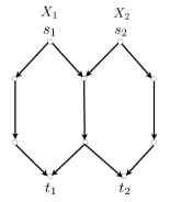
Figure 1: Example 1

Therefore, condition (3.1) in Theorem 3.1 is satisfied with equality, so that the sourse is transmissible over the network. Then, how to attain this transmissibility? That is depicted in Fig.2 where $\oplus$ denotes the exclusive OR. Fig. 3 depicts the corresponding capacity region, which is within the framework of the previous work (e.g., see Ahlswede et al. [1]).

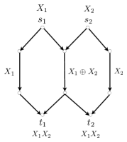
Figure 2: Coding for Example 1

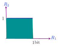
Figure 3: Capacity region for Example 1

Example 2.  Consider the network with noisy channels as in Fig.4 where the solid edges have capacity 1 and the broken edges have capacity $h(p)<1$. Here, $h(p)$ ($0<p<\frac{1}{2}$) is the binary entropy defined by $h(p)=-p\log_{2}p-(1-p)\log_{2}(1-p).$ The source $(X_{1},X_{2})$ generated at the nodes $s_{1},s_{2}$ is the binary symmetric source with crossover probability $p$, i.e.,

$$\Pr\{X_{1}=1\}=\Pr\{X_{1}=0\}=\Pr\{X_{2}=1\}=\Pr\{X_{2}=0\}=\frac{1}{2},$$

$$\Pr\{X_{2}=1|X_{1}=0\}=\Pr\{X_{2}=0|X_{1}=1\}=p.$$

Notice that $X_{1},X_{2}$ are not independent. The capacity function of this network is computed as follows:

$$\rho_{t_{1}}(\{s_{2}\}) = \rho_{t_{2}}(\{s_{1}\})=h(p),$$

$$\rho_{t_{1}}(\{s_{1}\}) = \rho_{t_{2}}(\{s_{2}\})=1+h(p),$$

$$\rho_{t_{1}}(\{s_{1},s_{2}\}) = \rho_{t_{2}}(\{s_{1},s_{2}\})=2;$$

$$\rho_{{\cal N}}(\{s_{2}\}) = \min(\rho_{t_{1}}(\{s_{2}\}),\rho_{t_{2}}(\{s_{2}\}))=h(p),$$

$$\rho_{{\cal N}}(\{s_{1}\}) = \min(\rho_{t_{1}}(\{s_{1}\}),\rho_{t_{2}}(\{s_{1}\}))=h(p),$$

$$\rho_{{\cal N}}(\{s_{1},s_{2}\}) = \min(\rho_{t_{1}}(\{s_{1},s_{2}\}),\rho_{t_{2}}(\{s_{1},s_{2}\}))=2.$$

On the other hand,

$$H(X_{1}|X_{2}) = h(p),$$

$$H(X_{2}|X_{1}) = h(p),$$

$$H(X_{1}X_{2}) = 1+h(p).$$

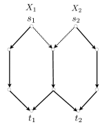
Figure 4: Example 2

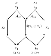
Figure 5: Coding for Example 2

Therefore, condition (3.1) in Theorem 3.1 is satisfied with strict inequality, so that the source is transmissible over the network. Then, how to attain this transmissibility? That is depicted in Fig.5 where ${\bf x}_{1},{\bf x}_{2}$ are $n$ independent copies of $X_{1},X_{2}$, respectively, and $A$ is an $m\times n$ matrix ($m=nh(p)<n)$. Notice that the entropy of ${\bf x}_{1}\oplus{\bf x}_{2}$ (componentwise exclusive OR) is $nh(p)$ bits and hence it is possible to recover ${\bf x}_{1}\oplus{\bf x}_{2}$ from $A({\bf x}_{1}\oplus{\bf x}_{2})$ (of length $m=nh(p)$) with asymtoticaly negligible probability of decoding error, provided that $A$ is appropriately chosen (see Körner and Marton [20]). It should be remarked that this example cannot be justified by the previous works such as Ho et al. [13], Ho et al. [14], and Ramamoorthy et al. [15], because all of them assume noiseless channels with capacity of one bit, i.e., this example is outside the previous framework.

5 Alternative Transmissibility Condition

In this section we demonstrate an alternative transmissibility condition equivalent to the necessary and sufficient condition (3.1) given in Theorem 3.1.

To do so, for each $t\in\Psi$ we define the polyhedron ${\cal C}_{t}$ as the set of all nonnegative rates $(R_{s};s\in\Phi)$ such that

$$\sum_{i\in S}R_{i}\leq\rho_{t}(S)\quad(\emptyset\neq\forall S\subset\Phi),$$ (5.1)

where $\rho_{t}(S)$ is the capacity function as defined in (2.16) of Section 2. Moreover, define the polyhedron ${\cal R}_{\mbox{{\scriptsize SW}}}$ as the set of all nonnegative rates $(R_{s};s\in\Phi)$ such that

$$H(X_{S}|X_{\overline{S}})\leq\sum_{i\in S}R_{i}\quad(\emptyset\neq\forall S\subset\Phi),$$ (5.2)

where $H(X_{S}|X_{\overline{S}})$ is the conditional entropy rate as defined in Section 2. Then, we have the following theorem on the transmissibility over the network ${\cal N}=(V,E,C)$.

Theorem 5.1

The following two statements are equivalent:

$$1) H(X_{S}|X_{\overline{S}})\leq\rho_{{\cal N}}(S)\quad(\emptyset\neq\forall S\subset\Phi),$$ (5.3)

$$2) {\cal R}_{\mbox{{\scriptsize SW}}}\cap{\cal C}_{t}\neq\emptyset\quad(\forall t\in\Psi).$$ (5.4)

In order to prove Theorem 5.1 we need the following lemma:

Lemma 5.1 (Han [3])

Let $\sigma(S)$, $\rho(S)$ be a co-polymatroid and a polymatroid, respectively, as defined in Remark 2.3. Then, the necessary and sufficient condition for the existence of some nonnegative rates $(R_{s};s\in\Phi)$ such that

$$\sigma(S)\leq\sum_{i\in S}R_{i}\leq\rho(S)\quad(\emptyset\neq\forall S\subset\Phi)$$ (5.5)

is that

$$\sigma(S)\leq\rho(S)\quad(\emptyset\neq\forall S\subset\Phi).$$ (5.6)

$\Box$

Proof of Theorem 5.1 :

Suppose that (5.3 ) holds, then, in view of (2.17), this implies

$$H(X_{S}|X_{\overline{S}})\leq\rho_{t}(S)\quad(\forall t\in\Psi,\emptyset\neq\forall S\subset\Phi).$$ (5.7)

Since, as was pointed out in Remark 2.3, $\sigma(S)=H(X_{S}|X_{\overline{S}})$ and $\rho(S)=\rho_{t}(S)$ are a co-polymatroid and a polymatroid, respectively, application of Lemma 5.1 ensures the existence of some nonnegative rates $(R_{s};s\in\Phi)$ such that

$$H(X_{S}|X_{\overline{S}})\leq\sum_{i\in S}R_{i}\leq\rho_{t}(S)\quad(\forall t\in\Psi,\emptyset\neq\forall S\subset\Phi),$$ (5.8)

which is nothing but (5.4).

Next, suppose that (5.4) holds. This implies (5.8), which in turn implies (5.7), i.e., (5.3) holds. $\Box$

Remark 5.1

The necessary and sufficient condition of the form (5.4) appears (without the proof) in Ramamoorthy, Jain, Chou and Effros [15] with $|\Phi|=2,|\Psi|=2$, which they call the feasibility. They attribute the sufficiency part simply to Ho, Médard, Effros and Koetter [13] with $|\Phi|=2,|\Psi|=1$ (also, cf. Ho, Médard, Koetter, Karger, Effros, Shi, and Leong [14] with $|\Phi|=2,|\Psi|=1$), while attributing the necessity part to Han [3], Barros and Servetto [9]. However, notice that all the arguments in [13], [14] ([13] is included in [14]) can be validated only within the class of stationary memoryless sources of integer bit rates and error-free channels (i.e., the identity mappings) all with one bit capacity (this restriction is needed to invoke “Menger’s theorem” in graph theory); while the present paper, without such severe restrictions, treats “general” acyclic networks, allowing for general correlated stationary ergodic sources as well as general statistically independent channels with each satisfying the strong converse property (cf. Lemma 2.1). Moreover, as long as we are concerned also with noisy channels, the way of approaching the problem as in [13], [14] does not work as well, because in this noisy case we have to cope with two kinds of error probabilities, one due to error probabilities for source coding and the other due to error probabilities for network coding (i.e., channel coding); thus in the noisy channel case or in the noiseless channel case with non-integer capacities and/or i.i.d. sources of non-integer bit rates, [15] cannot attribute the sufficiency part of (5.4) to [13], [14].

It should be noted here also that [13] and [14], though demonstrating relevant error exponents (the direct part), do not have the converse part. $\Box$

Remark 5.2 (Separation)

Here, the term of separation is used to mean separation of distributed source coding and network coding with independent sources. Theorem 3.1 does not immediately guarantee separation in this sense. However, when $\rho_{{\cal N}}(S)$ is, for example, a polymatroid as mentioned in Remark 2.3, separation in this sense is ensured, because in this case it is guaranteed by Lemma 5.1 that there exist some nonnegative rates $R_{i}$ $(i\in\Phi)$ such that

$$H(X_{S}|X_{\overline{S}})\leq\sum_{i\in S}R_{i}\leq\rho_{{\cal N}}(S)\quad(\emptyset\neq\forall S\subset\Phi).$$ (5.9)

Then, the first inequality ensures reliable distributed source coding by virtue of the theorem of Slepian and Wolf (cf. Cover [5]), while the second inequality ensures reliable network coding, that looks like for non-physical flows, with independent distributed sources of rates $R_{i}$ ($i\in\Phi$; see Remark 3.2). Furthermore, in the particular case of $|\Psi|=1$, the capacity function $\rho_{{\cal N}}(S)$ is always a polymatroid, so separation holds, where network coding looks like for physical flows (cf. Han [3], Meggido [23], and Ramamoorthy, Jain, Chou and Effros [15]). Then, it would be natural to ask the question whether separability in this sense implies polymatroidal property. In this connection, [15] claims that, in the case with $|\Phi|=|\Psi|=2$ and with rational capacities as well as sources of integer bit rates, “separation” always holds, irrespective of the polymatroidal property, while in the case of $|\Phi|>2$ or $|\Psi|>2$ no conclusive claim is not made. On the other hand, we notice here that condition (5.9) is actually sufficient for separability despite the non-polymatroid property of $\rho_{{\cal N}}(S)$. Condition (5.9) is equivalently written as

$${{\cal R}_{\mbox{{\scriptsize SW}}}\cap\left(\bigcap_{t\in\Psi}{\cal C}_{t}\right)\neq\emptyset}$$ (5.10)

for any general network ${\cal N}$. Moreover, in view of Remark 3.2, it is not difficult to check that (5.10) is also necessary. Thus, our conclusion is that, in general, condition (5.10) is not only sufficient but also necessary for separability. $\Box$

Remark 5.3

It is possible also to consider network coding with cost. In this regard the reader may refer to, e.g., Han [3], Ramamoorthy [27], Lee et al. [28]. $\Box$

Remark 5.4

So far we have focused on the case where the channels of a network are quite general but are statistically independent. On the other hand, we may think of the case where the channels are not necessarily statistically independent. This problem is quite hard in general. A typical tractable example of such networks would be a class of acyclic deterministic relay networks with no interference (called the Aref network) in which the concept of “channel capacity” is irrelevant. In this connection, Ratnakar and Kramer [24] have studied Aref networks with a single source and multiple sinks, while Korada and Vasudevan [25] have studied Aref networks with multiple correlated sources and multiple sinks. The network capacity formula as well as the network matching formula obtained by them are in nice correspondence with the formula obtained by Ahlswede et al. [1] as well as Theorem 3.1 established in this paper, respectively. $\Box$

References

• [1] R. Ahlswede, N.Cai, S.Y. R. Li and R.W.Yeung, “Network information flow,” IEEE Transactions on Information Theory, vol.IT-46, no.4, pp. 1204-1216, 2000
• [2] R.W. Yeung, A First Course in Information Theory, Kluwer, 2002
• [3] T.S. Han, “Slepian-Wolf-Cover theorem for a network of channels,” Information and Control, vol.47, no.1, pp. 67-83, 1980
• [4] T.S. Han, Information-Spectrum Methods in Information Theory, Springer-verlag, Berlin, 2003
• [5] T. M. Cover, “A simple proof of the data compression theorem of Slepian and Wolf for ergodic sources,” IEEE Transactions on Information Theory, vol.IT-21, pp. 226-228, 1975
• [6] S. Verdú and T.S.Han, “A general formula for channel capacity,” IEEE Transactions on Information Theory, vol.IT-40, no.4, pp.1147-1157, 1994
• [7] R. G. Gallager, Information Theory and Reliable Communication, Wiley, New York,1968
• [8] T. M. Cover and J. A. Thomas, Elements of Information Theory, Wiley, New York, 1991
• [9] J. Barros and S. D. Servetto, “Network information flow with correlated sources,” IEEE Transactions on Information Theory, vol.IT-52, no.1, pp.155-170, 2006
• [10] L. Song, R.W.Yeung and N.Cai, “A separation theorem for single-source network coding,” IEEE Transactions on Information Theory, vol.IT-52, no.5, pp.1861-1871, 2006
• [11] X. Yan, R.W.Yeung and Z. Zhang, “The capacity region for multiple-source multiple-sink network coding,” Proc. IEEE International Symposium on Information Theory, June 2007
• [12] L. Song, R.W. Yeung and N.Cai, “Zero-error network coding for acyclic networks,” IEEE Transactions on Information Theory, vol.IT-49, no.12, pp.3129-3139, 2003
• [13] T. Ho, M. Médard, M.Effros and R. Koetter, “Network coding for correlated sources,” Proc. Conference on Information Science and Systems, 2004
• [14] T. Ho, M. Médard, and R. Koetter, D.R.Karger, M.Effros, Jun Shi, and Ben Leong, “A random linear network coding approach to multicast,” IEEE Transactions on Information Theory, vol.IT-52, no.10, pp.4413-4430, 2006
• [15] A. Ramamoorthy, K. Jain, A. Chou and M.Effros, “Separating distributed source coding from network coding,” IEEE Transactions on Information Theory, vol.IT-52, no.6, pp.2785-2795, 2006
• [16] R. Koetter and M. Medárd, “An algebraic approach to network coding,” IEEE Transactions on Information Theory, vol.IT-49, no.5, pp.782-795, 2003
• [17] A. Li and R.W. Yeung, “Network information flow - multiple source,” IEEE International Symposium on Information Theory, 2001
• [18] X. Zhang, Jun Chen, S. B. Wicker and T. Berger, “Successive coding in multiuser information theory,” IEEE Transactions on Information Theory, vol.IT-53, no.6, pp.2246-2254, 2007
• [19] I. Csiszár, “Linear codes for sources and source networks: error exponents, universal coding,” IEEE Transactions on Information Theory, vol.IT-28, no.4, pp.585-592, 1982
• [20] J. Körner and Marton, “How to encode the modulo-two sum of binary sources,” IEEE Transactions on Information Theory, vol.IT-25, pp. 219-221, 1979
• [21] I. Csiszár and J. Körner, Information Theory: Coding Theorems for Discrete Memoryless Systems, Academic Press, New York, 1981
• [22] X. Yan, J. Yang and Z. Zhang, “An outer bound for multiple source multiple sink coding with minimum cost consideration,” IEEE Transactions on Information Theory, vol.IT-52, no.6, pp. 2373-2385, 2006
• [23] N. Meggido, “Optimal flows in networks with multiple sources and multiple sinks,” Mathematical Programming, vol.7, pp.97-107, 1974
• [24] N. Ratnakar and G. Kramer, “The multicast capacity of deterministic relay networks with no interference, h IEEE Trans. Inform. Theory, vol. 52, no. 6, pp.2425-2432, Jun. 2006.
• [25] S. B. Korada and D. Vasudevan, “Broadcast and Slepian-Wolf multicast over Aref networks,” Proc. IEEE International Symposium on Information Theory, pp. 1656-1660, Toronto, Canada, July 6-11, 2008
• [26] S. Avestimehr Wireless network information flow, PhD thesis, University of California, Berkeley, 2008
• [27] A. Ramamoorthy, “Minimum cost distributed source coding over a network,” Proc. IEEE International Symposium on Information Theory, Nice, France, 2007
• [28] A. Lee, M.Medárd, K.Z. Haigh, S. Gowan, and P. Rupel “Minimum-cost subgraphs for joint distributed source and network coding,” Thirs Workshop on Network Coding, Theory, and Applications, January 2007