ANL-HEP-PR-08-80 EFI-08-31 FERMILAB-PUB-08-562-T Gauge-Higgs Unification, Neutrino Masses and
Dark Matter in Warped Extra Dimensions

Abstract

Gauge Higgs Unification in Warped Extra Dimensions provides an attractive solution to the hierarchy problem. The extension of the Standard Model gauge symmetry to $SO(5)\times U(1)_{X}$ allows the incorporation of the custodial symmetry $SU(2)_{R}$ plus a Higgs boson doublet with the right quantum numbers under the gauge group. In the minimal model, the Higgs mass is in the range 110–150 GeV, while a light Kaluza Klein (KK) excitation of the top quark appears in the spectrum, providing agreement with precision electroweak measurements and a possible test of the model at a high luminosity LHC. The extension of the model to the lepton sector has several interesting features. We discuss the conditions necessary to obtain realistic charged lepton and neutrino masses. After the addition of an exchange symmetry in the bulk, we show that the odd neutrino KK modes provide a realistic dark matter candidate, with a mass of the order of 1 TeV, which will be probed by direct dark matter detection experiments in the near future.

1 Introduction

Warped Extra Dimensions present an elegant solution to the hierarchy problem, where all fundamental parameters are of the order of the Planck scale. The weak scale–Planck scale hierarchy is obtained by an exponential warp factor, which is naturally small provided the Higgs field is localized towards the so-called infrared brane [1]. If all Standard Model (SM) fields propagate in the bulk, the theory leads to the presence of Kaluza Klein (KK) modes which tend to be localized towards the IR brane and therefore couple sizably to the Higgs. This in turn leads to large mixing between the heavy SM particles and their KK modes, leading to modifications of the electroweak parameters and therefore to strong constraints from electroweak precision measurements [2]–[7]. These constraints may be weakened by the introduction of brane kinetic terms [8]–[11] or custodial symmetries [12], [13], which allow the presence of KK modes with masses of the order of a few TeV.

One of the attractive features of these models is the natural explanation of the hierarchy of fermion masses by the localization of the fermion fields in the bulk [16]–[18]. The chiral properties of the fermions are obtained by imposing an orbifold symmetry and demanding that the fields are odd or even under such a symmetry. Fermion fields that are even under the orbifold symmetry at the infrared and ultraviolet branes present zero modes, which are chiral and therefore may be identified with the SM fermion fields. The localization of the zero modes is governed by the bulk mass parameter $ck$, with $k$ the curvature of the extra dimension and $c$, a number of order one. While the zero modes of chiral fields with $c>1/2$ couple weakly to the Higgs and are therefore light, the heavy SM fields are associated with bulk mass parameters $c\leq 1/2$. Due to the exponential behavior of the zero mode wave functions, large hierarchies between the fermion masses are generated by small variations of the corresponding $c$-parameters.

Gauge Higgs Unification models identify the Higgs field with the five dimensional component of the gauge fields [19]. An extended gauge symmetry is necessary for the successful implementation of this mechanism. In particular, models based on the gauge group $SO(5)\times U(1)_{X}$ include the custodial and weak gauge symmetry via $SO(5)\supset SO(4)\equiv SU(2)_{L}\times SU(2)_{R}$ [20],[21] [22]. Moreover, provided the $SO(5)$ symmetry is broken to a subgroup of $SO(4)$ by boundary conditions at both branes, the fifth dimensional components of $SO(5)/SO(4)$ have the proper quantum numbers to be identified with the Higgs field, which is exponentially localized towards the IR brane.

Since the Higgs originates from gauge fields, its tree level potential vanishes. In a previous work [25], we computed the one-loop effective potential and demonstrated that electroweak symmetry breaking, with the proper generation of third generation quark and gauge boson masses may be obtained for the same values of the bulk mass parameters that lead to agreement with precision electroweak data at the one-loop level. Moreover, we showed that the Higgs mass is in the range 110–150 GeV and that a light KK mode of the top quark, $T^{\prime}$, appears in the spectrum, with a mass small enough so that the KK gluon may decay into it. The presence of this light KK mode has a strong impact on the phenomenology of the model [26]. For instance, searches for the KK gluon by its decay into top-quarks [27],[28], [29] is rendered difficult due to the presence of the additional dominant decay mode into KK top-quarks and the broadness of the KK gluon. On the contrary, the constructive interference between the QCD and KK gluon induced pair production of the top-quark KK mode allows to search for a $T^{\prime}$ for values of the masses much larger than those at reach in the case of just the QCD production cross section.

In this article, we will analyze the addition of the lepton sector in the gauge Higgs unification scenario. To add leptons, we will proceed in a similar way as for the quark sector. The left-handed leptons will be added in a fundamental representation of $SO(5)$, with $Q_{X}=0$, while the right-handed neutrino and charged lepton fields will be added in a fundamental representation and a $\bf{10}$ of $SO(5)$ also with charge $Q_{X}=0$, respectively.

Due to the gauge origin of the Higgs field, a possible local infrared brane operator $(LH)\;LH/M$, which could lead to large values of the neutrino Majorana masses, should come from the fifth dimensional component of the covariant derivative of the lepton fields and therefore can only naturally arise from the integration of the right-handed neutrinos, with a local IR Majorana mass. Indeed, since the fields associated with the right-handed neutrino zero modes are singlets under the conserved gauge groups on both the infrared and ultraviolet branes, one can always add Majorana masses for these fields on the infrared and ultraviolet branes. We will therefore consider these masses and implement a See-Saw mechanism for the generation of the light neutrino masses [31],[32]. We will show how to incorporate these masses within the context of these models, obtain the modified profile functions and define the conditions to derive a realistic spectrum.

Furthermore, the introduction of an exchange symmetry [43], which is preserved in the bulk, yields a natural dark matter candidate in the spectrum, that may be identified with the odd KK modes of the right-handed neutrino. This exchange symmetry requires the identification of the bulk mass parameter of the dark matter candidate with the one of the right-handed neutrinos, establishing a connection between neutrino masses and the relic dark matter density. We will show that, if the odd fermions are assumed to be Dirac particles, the predicted relic density is the correct one for Dirac fermion masses of the order of 1 TeV. In the Majorana case, somewhat smaller masses are allowed, and the results depend on the relative values of the ultraviolet and infrared Majorana masses. We will show that in both the Dirac and Majorana cases, direct detection experiments will efficiently probe the existence of the proposed dark matter candidates.

The article is organized as follow: In section 2 we discuss the properties of leptons in scenarios of Gauge Higgs Unification. In section 3 we discuss the generation of charged lepton and neutrino masses. In section 4 we analyze the possibility of incorporating dark matter via an exchange bulk symmetry, analyzing the couplings and the annihilation diagrams, as well as the direct detection of these dark matter candidates. We reserve section 5 for our conclusions. Some technical details are given in the Appendix.

2 Leptons in Gauge Higgs Unification Scenarios

The goal of the current work is to add the lepton sector into the minimal Gauge Higgs Unification model described above, including right handed neutrinos, with brane Majorana masses. We will proceed in a similar way as in the quark case [25], and discuss the general question of charged lepton and neutrino mass generation.

Similar to the quark sector, we let the SM $SU(2)_{L}$ lepton doublet containing the left-handed charged leptons and neutrinos, $l_{L}$ and $\nu_{L}$, arise from a ${\bf 5}_{0}$ of $SO(5)\times U(1)_{X}$, where the subscript refers to the $U(1)_{X}$ charge. The right handed neutrino, $N_{R}$ will be included as the singlet component in a fundamental representation of $SO(5)$, while the right-handed charged lepton, $l_{R}$, is placed in a ${\bf 10}_{0}$ of $SO(5)$ analogously to the $d_{R}$. One may also include brane mass terms connecting different multiplet components, as well as new brane Majorana masses for the right handed neutrino $N_{R}$:

$$\Big{(}M_{UV}\delta(y)-M_{IR}\delta(y-L)\Big{)}N_{R}N_{R}.$$ (1)

The right handed neutrino, $N_{R}$, in principle could be identified with the singlet right-handed component in the same multiplet as the left-handed leptons. However, in order to naturally suppress lepton flavor violation effects and maintain agreement with precision electroweak measurements, the left-handed leptons should be localized towards the UV brane [14],[15]. The zero modes of the corresponding right-handed multiplet will therefore be localized towards the IR brane. This implies that even with a natural scale for the brane masses $\mathcal{O}(M_{Pl})$, the exponential suppression of the wave function at the UV brane would lead to a effective Majorana mass for $N_{R}$ which is much smaller than the Planck scale. This, in turn, after the implementation of the See-Saw mechanism, leads to too large values for the observed neutrino masses. Therefore, as we will discuss below, it will prove to be necessary to have the left-handed leptons in a different multiplet as the right-handed neutrinos.

If $N_{R}$ belongs to the same multiplet as the left-handed leptons:

$$\begin{array}[]{c}\begin{array}[]{ccccccc}\xi^{i}_{1L}&\sim&L^{i}_{1L}&=&\begin{pmatrix}\chi^{e_{i}}_{1L}(-,+)_{1}&l^{n_{i}}_{L}(+,+)_{0}\\ \chi^{n_{i}}_{1L}(-,+)_{0}&l^{e_{i}}_{L}(+,+)_{-1}\end{pmatrix}&\oplus&N^{i}_{L}(-,-)_{0}\leavevmode\nobreak\ ,\vspace{3mm}\\ \end{array}\end{array}\vspace{3mm}$$ (4)

$$\begin{array}[]{l}\xi^{i}_{2R}\sim\\ \\ \begin{array}[]{ccccccccccc}T^{i}_{1R}=\begin{pmatrix}\psi^{\prime i}_{R}(-,+)_{1}\\ N^{\prime i}_{R}(-,+)_{0}\\ E^{\prime i}_{R}(-,+)_{-1}\end{pmatrix}\oplus T^{i}_{2R}=\begin{pmatrix}\psi^{\prime\prime i}_{R}(-,+)_{1}\\ N^{\prime\prime i}_{R}(-,+)_{0}\\ E^{i}_{R}(+,+)_{-1}\end{pmatrix}\oplus L^{i}_{2R}=\begin{pmatrix}\chi^{e_{i}}_{2R}(-,+)_{1}&l^{\prime\prime n_{i}}_{R}(-,+)_{0}\\ \chi^{n_{i}}_{2R}(-,+)_{0}&l^{\prime\prime e_{i}}_{R}(-,+)_{-1}\end{pmatrix},\end{array}\end{array}$$ (9)

Alternatively, the right-handed neutrino can be incorporated in a different multiplet from the left-handed lepton one. The two multiplet assignments are as follows:

$$\begin{array}[]{c}\begin{array}[]{ccccccc}\xi^{i}_{1L}&\sim&L^{i}_{1L}&=&\begin{pmatrix}\chi^{e_{i}}_{1L}(-,+)_{1}&l^{n_{i}}_{L}(+,+)_{0}\\ \chi^{n_{i}}_{1L}(-,+)_{0}&l^{e_{i}}_{L}(+,+)_{-1}\end{pmatrix}&\oplus&N^{\prime i}_{L}(-,+)_{0}\leavevmode\nobreak\ ,\vspace{3mm}\\ \xi^{i}_{2R}&\sim&L^{i}_{2R}&=&\begin{pmatrix}\chi^{e_{i}}_{2R}(-,+)_{1}&l^{\prime{n_{i}}}_{R}(-,+)_{0}\\ \chi^{n_{i}}_{2R}(-,+)_{0}&l^{\prime{e_{i}}}_{R}(-,+)_{-1}\end{pmatrix}&\oplus&N^{i}_{R}(+,+)_{0}\leavevmode\nobreak\ ,\end{array}\end{array}\vspace{3mm}$$ (13)

$$\begin{array}[]{l}\xi^{i}_{3R}\sim\\ \\ \begin{array}[]{ccccccccccc}T^{i}_{1R}=\begin{pmatrix}\psi^{\prime i}_{R}(-,+)_{1}\\ N^{\prime i}_{R}(-,+)_{0}\\ E^{\prime i}_{R}(-,+)_{-1}\end{pmatrix}\oplus T^{i}_{2R}=\begin{pmatrix}\psi^{\prime\prime i}_{R}(-,+)_{1}\\ N^{\prime\prime i}_{R}(-,+)_{0}\\ E^{i}_{R}(+,+)_{-1}\end{pmatrix}\oplus L^{i}_{3R}=\begin{pmatrix}\chi^{e_{i}}_{3R}(-,+)_{1}&l^{\prime\prime n_{i}}_{R}(-,+)_{0}\\ \chi^{n_{i}}_{3R}(-,+)_{0}&l^{\prime\prime e_{i}}_{R}(-,+)_{-1}\end{pmatrix},\end{array}\end{array}$$ (18)

where we show the decomposition under $SU(2)_{L}\times SU(2)_{R}$, and explicitly write the $U(1)_{EM}$ charges. The $L^{i}$s are bidoublets of $SU(2)_{L}\times SU(2)_{R}$, with $SU(2)_{L}$ acting vertically and $SU(2)_{R}$ acting horizontally. The $T^{i}_{1}$’s and $T^{i}_{2}$’s transform as $({\bf 3},{\bf 1})$ and $({\bf 1},{\bf 3})$ under $SU(2)_{L}\times SU(2)_{R}$, respectively, while $N^{i}$ and $N^{\prime i}$ are $SU(2)_{L}\times SU(2)_{R}$ singlets. The superscripts, $i=1,2,3$, label the three generations.

We also show the parities on the indicated 4D chirality, where $-$ and $+$ stands for odd and even parity conditions and the first and second entries in the bracket correspond to the parities in the UV and IR branes respectively. Let us stress that while odd parity is equivalent to a Dirichlet boundary condition, the even parity is a linear combination of Neumann and Dirichlet boundary conditions, that is determined via the fermion bulk equations of motion as discussed below. The boundary conditions for the opposite chirality fermion multiplet can be read off the ones above by a flip in both chirality and boundary condition, for example $(-,+)_{L}\rightarrow(+,-)_{R}$. In the absence of mixing among multiplets satisfying different boundary conditions, the SM fermions arise as the zero-modes of the fields obeying $(+,+)$ boundary conditions. The remaining boundary conditions are chosen so that $SU(2)_{L}\times SU(2)_{R}$ is preserved on the IR brane and so that mass mixing terms, necessary to obtain the SM fermion masses after EW symmetry breaking, can be written on the IR brane. Consistency of the above parity assignments with the original orbifold $Z_{2}$ symmetry at the IR brane was discussed in Appendix B of Ref. [25]. The three families will behave similarly, and therefore, we will drop the family indices and concentrate only on one lepton family. Large mixing angles in the lepton sector can be naturally obtained while suppressing lepton flavor changing neutral currents if the left-handed leptons have similar bulk mass parameters, $c^{i}_{1}$ [36],[37], and in the following we will assume them to be equal. We will return to this issue in section 3.3. The zero modes of the leptons are too light and too weakly coupled to the Higgs boson to affect the Higgs potential in any significant way. The lepton KK modes may be coupled more strongly to the Higgs, but their gauge invariant mass is much larger than the Higgs induced one and therefore they tend to contribute only weakly to both the Higgs potential and to precision electroweak observables.

One can add localized brane mass terms to the Lagrangian in both the one and the two multiplet cases:

$$\mathcal{L}_{1} = -2\delta(x_{5}-L)\Big{[}\bar{L}_{1L}M_{L_{2}}L_{2R}+\mathrm{h.c.}\Big{]}-\big{[}M_{IR}\delta(x_{5}-L)-M_{UV}\delta(x_{5})\Big{]}N_{R}N_{R}\leavevmode\nobreak\ ;$$ (19)

$$\mathcal{L}_{2} = -2\delta(x_{5}-L)\Big{[}\bar{N}^{\prime}_{L}M_{L_{1}}N_{R}+\bar{L}_{1L}M_{L_{2}}L_{3R}+\mathrm{h.c.}\Big{]}-\big{[}M_{IR}\delta(x_{5}-L)-M_{UV}\delta(x_{5})\Big{]}N_{R}N_{R}\leavevmode\nobreak\ .$$ (20)

With the introduction of the brane mixing terms, the different multiplets are now related via the equations of motion. The fermions, like the gauge bosons, can be expanded in their KK basis:

$$\psi_{L}(x,x_{5})=\sum_{n}f_{L,n}(x_{5},h)\psi_{L,n}(x),\quad\quad\psi_{R}(x,x_{5})=\sum_{n}f_{R,n}(x_{5},h)\psi_{R,n}(x).$$ (21)

Solving the equations of motion in the presence of $h$ becomes complicated, as the different modes are mixed. However, 5D gauge symmetry relates these solutions to solutions with $h=0$ [23], with $\Omega(x_{5},h)$, the gauge transformations that removes the vev of $h$:

$$\Omega(x_{5},h)=\exp\left[-iC_{h}hT^{4}\int_{0}^{x_{5}}dy\,a^{-2}(y)\right].$$ (22)

The form of the bulk profile functions at $h=0$ is given in Appendix A.

The boundary masses lead to a redefinition of the effective boundary conditions for the fermion fields at the branes. Let’s first analyze the case of a Dirac boundary mass term on the infrared brane, $M_{L}$, involving fields from different multiplets $\bar{\Psi}^{i}_{\rm L}\Psi^{j}_{\rm R}$, $i,j=1,2,3$ for the different multiplets. Quite generally, we shall call the profile of the left-handed field and the right-handed field participating in the mass term $g_{\rm L}$ and $h_{\rm R}$, respectively. The right handed component, $\Psi^{i}_{R}$ with profile function $g_{R}$ and the left-handed component $\Psi^{j}_{L}$ with profile function $h_{L}$ have Dirichlet boundary conditions on the brane, and therefore $g_{R}(L)=h_{L}(L)=0$. The equations of motion of the fields are affected by the localized masses, which induce a discontinuity on the odd-parity profile functions at the infrared brane. Indeed, keeping only the relevant terms, the integration of the equation of motion leads to

$$\int^{L+\epsilon}_{L-\epsilon}(\partial_{5}g_{R})dx_{5}=\int^{L+\epsilon}_{L-\epsilon}2M_{L}h_{R}\;\delta(x_{5}-L)dx_{5}.$$ (23)

Therefore, we obtain:

$$\lim_{\epsilon\rightarrow 0}g_{R}(L-\epsilon)=-M_{L}h_{R}(L),$$ (24)

and, similarly for the $h_{L}$

$$\lim_{\epsilon\rightarrow 0}h_{L}(L-\epsilon)=M_{L_{2}}g_{L}(L).$$ (25)

Eq. (24) and  (25) can now be reinterpreted as the new boundary conditions for the profiles at the IR brane.

Analogously, one can analyze the effect of the Majorana boundary mass, $M_{i}$, where $i=IR$ or $UV$. Let’s take the specific case of the field $N_{R}$, with a profile function $h_{R}$. Its chiral partner will have a profile function $h_{L}$ having an odd parity profile on both branes. The equation of motion in the presence of both the Majorana masses and the Dirac mass term $M_{L_{1}}$ leads to the following relationship

$$\int^{y+\epsilon}_{y-\epsilon}(\partial_{5}h_{L})dx_{5}=\int^{y+\epsilon}_{y-\epsilon}\Big{[}(\pm 2M_{i}h_{R}-h_{L})\delta(x_{5}-y)-2M_{L_{1}}g_{L}\delta(x_{5}-L)\Big{]}dx_{5}.$$ (26)

where the minus and plus signs are associated with the boundary conditions at $y=L$, and $y=0$, respectively. The odd parity at the branes then implies a Dirichlet boundary condition for the function $h_{L}$, which as before will present a discontinuity at the brane. For the IR boundary conditions we obtain:

$$\lim_{\epsilon\rightarrow 0}h_{L}(L-\epsilon)=M_{IR}h_{R}(L)+M_{L_{1}}g_{L}(L).$$ (27)

For the UV boundary condition, instead:

$$\lim_{\epsilon\rightarrow 0}h_{L}(0+\epsilon)=M_{UV}h_{R}(0).$$ (28)

Eq. (27-28) can now be reinterpreted as the new boundary condition for the profiles at the branes. The generalization of these expressions to the general case is straightforward.

2.1 Wave Functions in the Presence of UV Majorana Masses

The wave functions defined in Appendix A, $\tilde{S}_{M}$ and $\tilde{S}_{-M}$ are associated with Dirichlet boundary conditions at the ultraviolet brane for the left-handed and right-handed fields, respectively. In the presence of ultraviolet Majorana masses, however, the boundary conditions for the singlet component of the fundamental multiplets of $SO(5)$ read

$$f^{5}_{i,L}(0,0)=M_{UV}f^{5}_{i,R}(0,0)$$ (29)

where $i=1,2$ refers to the particular multiplet under analysis. In order to derive the profile function of these fields, let us first redefine the functions $a^{3/2}f_{L,R}\to f_{L,R}$ where $a=\exp(-kx_{5})$. With this redefinition, these functions satisfy the naive normalization condition,

$$\int_{0}^{L}dx_{5}\;f_{n}f_{m}=\delta_{m,n}.$$ (30)

The general solution for $f_{L}$ is given by:

$$f_{L}(x_{5},0)=Aa^{(c-1/2)}\tilde{S}_{M}+B\left(\frac{a}{z}\right)a^{-(c+1/2)}\tilde{S}_{-M}^{\prime}.$$ (31)

where $z$ is the associated particle mass. Defining

$$\tilde{f}_{L,R}=a^{-(c-1/2)}f_{L,R},$$ (32)

$\tilde{f}_{L,R}$ satisfy the simple equation of motion,

$$\tilde{f}_{R,L}(x_{5},0)=\mp\frac{a}{z}\partial_{5}\tilde{f}_{L,R}(x_{5},0).$$ (33)

Now, using Eq. (33), one obtains

$$\tilde{f_{R}}(x_{5},0) = -\frac{a}{z}\left(A\tilde{S}_{M}^{\prime}-B\left(\frac{a}{z}\right)a^{-2c}\left((1-2c)k\tilde{S}_{-M}^{\prime}-\tilde{S}_{-M}^{\prime\prime}\right)\right).$$ (34)

The second derivative functions may be replaced by means of the equation of motion of the fermion fields, namely

$$\tilde{S}_{-M}^{\prime\prime}=k(1-2c)\tilde{S}_{-M}^{\prime}-\frac{z^{2}}{a^{2}}\tilde{S}_{-M}.$$ (35)

We therefore see that $\tilde{f_{R}}$ reduces to:

$$\tilde{f_{R}}(x_{5},0)=Ba^{-2c}\tilde{S}_{-M}-A\frac{a}{z}\tilde{S}_{M}^{\prime}.$$ (36)

Rewriting these in terms of the $\dot{\tilde{S}}$ rather than $\tilde{S}^{\prime}$, with $\dot{\tilde{S}}_{\pm M}=\mp\frac{a(x_{5})}{z}\tilde{S}^{\prime}_{\pm M}$, we obtain

$$\tilde{f_{L}}(x_{5},0) = A\tilde{S}_{M}+Ba^{-2c}\dot{\tilde{S}}_{-M}$$ (37)

$$\tilde{f_{R}}(x_{5},0) = Ba^{-2c}\tilde{S}_{-M}+A\dot{\tilde{S}}_{M}$$ (38)

To solve for $A$ in terms of $B$, we need to use the UV boundary condition induced by the UV Majorana mass for $N_{R}$, Eq. (29):

$$Ba^{-2c}\dot{\tilde{S}}_{-M}(0) = AM_{UV}\dot{\tilde{S}}_{M}(0)$$

$$A = B\frac{a^{-2c}}{M_{UV}}\frac{\dot{\tilde{S}}_{-M}}{\dot{\tilde{S}}_{M}}|_{x_{5}=0}$$

$$\mathrm{since}\quad a=1\quad\mathrm{and}\quad\tilde{S}^{\prime}_{\pm M}(0,z)=z\quad\mathrm{for}\quad x_{5}=0\mathrm{:}$$

$$A = -\frac{B}{M_{UV}}.$$ (39)

Therefore, with the coefficients $A$ and $B$ as calculated above, the singlet functions become

$$f^{5}_{1,L}(x_{5},0) = C_{5}(S_{M_{1}}-M_{UV}\dot{S}_{-M_{1}})$$ (40)

$$f^{5}_{1,R}(x_{5},0) = C_{5}(-M_{UV}S_{-M_{1}}+\dot{S}_{M_{1}})$$ (41)

in the case of a single multiplet containing the left- and right-handed neutrinos, and

$$f^{5}_{2,L}(x_{5},0) = C_{10}(S_{M_{2}}-M_{UV}\dot{S}_{-M_{2}})$$ (42)

$$f^{5}_{2,R}(x_{5},0) = C_{10}(-M_{UV}S_{-M_{2}}+\dot{S}_{M_{2}})$$ (43)

in the case of two multiplets, where $S_{\pm M}=a^{(\pm c-1/2)}\tilde{S}_{\pm M}$ and $\dot{S}_{\pm M}=a^{(\pm c-1/2)}\dot{\tilde{S}}_{\pm M}$. Therefore, the fermion multiplets with $h=0$ take the form

$$\begin{array}[]{c}f_{1,L}(x_{5},0)=\left[\begin{array}[]{c}C_{1}S_{M_{1}}\\ C_{2}S_{M_{1}}\\ C_{3}\dot{S}_{-M_{1}}\\ C_{4}\dot{S}_{-M_{1}}\\ f^{5}_{1,L}\end{array}\right]\\ \\ \end{array} f_{3,R}(x_{5},0)=\left[\begin{array}[]{c}C_{11}S_{-M_{3}}\\ C_{12}S_{-M_{3}}\\ C_{13}S_{-M_{3}}\\ C_{14}S_{-M_{3}}\\ C_{15}S_{-M_{3}}\\ C_{16}S_{-M_{3}}\\ C_{17}S_{-M_{3}}\\ C_{18}S_{-M_{3}}\\ C_{19}S_{-M_{3}}\\ C_{20}\dot{S}_{M_{3}}\end{array}\right]$$ (61)

in the case of a single multiplet containing the left-handed and right-handed neutrinos, and

$$\begin{array}[]{c}f_{1,L}(x_{5},0)=\left[\begin{array}[]{c}C_{1}S_{M_{1}}\\ C_{2}S_{M_{1}}\\ C_{3}\dot{S}_{-M_{1}}\\ C_{4}\dot{S}_{-M_{1}}\\ C_{5}S_{M_{1}}\end{array}\right]\\ \\ \\ f_{2,L}(x_{5},0)=\left[\begin{array}[]{c}C_{6}\dot{S}_{-M_{2}}\\ C_{7}\dot{S}_{-M_{2}}\\ C_{8}\dot{S}_{-M_{2}}\\ C_{9}\dot{S}_{-M_{2}}\\ f^{5}_{2,L}\end{array}\right]\end{array} f_{3,R}(x_{5},0)=\left[\begin{array}[]{c}C_{11}S_{-M_{3}}\\ C_{12}S_{-M_{3}}\\ C_{13}S_{-M_{3}}\\ C_{14}S_{-M_{3}}\\ C_{15}S_{-M_{3}}\\ C_{16}S_{-M_{3}}\\ C_{17}S_{-M_{3}}\\ C_{18}S_{-M_{3}}\\ C_{19}S_{-M_{3}}\\ C_{20}\dot{S}_{M_{3}}\end{array}\right]$$ (86)

in the two multiplet case, where the $C_{i}$ are normalization constants.

3 Lepton Spectrum

Applying the boundary conditions at $x_{5}=L$, taking into account the mass mixing terms from Eqs. (19) and (20) and using the procedure defined in Eqs. (24)–(27), we derive the conditions on the lepton wave functions $f(L,h)$ in the presence of the Higgs field. In the case of only one multiplet containing both the left-handed and right-handed neutrinos one gets the following conditions at the IR brane:

$$\begin{array}[]{ccc}f_{1,R}^{1,...,4}+M_{L_{2}}f_{3,R}^{1,...,4}=0&&f_{1,L}^{5}-M_{IR}f_{1,R}^{5}=0\\ &&\\ f_{3,L}^{1,...,4}-M_{L_{2}}f_{1,L}^{1,...,4}=0&&f_{3,L}^{5,...,10}=0\end{array}$$ (90)

In the two multiplets, instead, one obtains:

$$\begin{array}[]{ccccc}f_{1,R}^{1,...,4}+M_{L_{2}}f_{3,R}^{1,...,4}=0&&f_{1,R}^{5}+M_{L_{1}}f_{2,R}^{5}=0&&f_{2,L}^{1,...,4}=0\\ &&&&\\ f_{3,L}^{1,...,4}-M_{L_{2}}f_{1,L}^{1,...,4}=0&&f_{2,L}^{5}-M_{L_{1}}f_{1,L}^{5}-M_{IR}f_{2,R}^{5}=0&&f_{3,L}^{5,...,10}=0\end{array}$$ (94)

where the superscripts denote the vector components.

This defines a system of linear equations for the normalization constants $C_{i}$. Asking that the determinant of the functional coefficients of this system vanishes in order to get a non-trivial solution [24], one obtains the following relations:

$$\dot{\tilde{S}}_{-M_{3}}^{5}=0$$ (95)

$$M_{L_{2}}^{2}\tilde{S}_{M_{1}}\tilde{S}_{-M_{3}}+\dot{\tilde{S}}_{M_{1}}\dot{\tilde{S}}_{-M_{3}}=0$$ (96)

$$2\tilde{S}_{M_{3}}\left[M_{L_{2}}^{2}\tilde{S}_{-M_{3}}\dot{\tilde{S}}_{-M_{1}}+\tilde{S}_{-M_{1}}\dot{\tilde{S}}_{-M_{3}}\right]-M_{L_{2}}^{2}\dot{\tilde{S}}_{-M_{1}}\sin\left[\frac{\lambda h}{f_{h}}\right]^{2}=0$$ (97)

$$2\left[-M_{L_{2}}^{4}\tilde{S}_{M_{1}}\tilde{S}_{-M_{3}}^{2}\left[\dot{\tilde{S}}_{-M_{1}}(\tilde{S}_{M_{1}}-e^{2c_{1}kL}M_{UV}\dot{\tilde{S}}_{-M_{1}})+M_{IR}(1-\tilde{S}_{M_{1}}\tilde{S}_{-M_{1}}+e^{2c_{1}kL}M_{UV}\tilde{S}_{-M_{1}}\dot{\tilde{S}}_{-M_{1}})\right]\right.$$

$$-M_{L_{2}}^{2}\tilde{S}_{-M_{3}}\left[2\tilde{S}_{M_{1}}^{2}\tilde{S}_{-M_{1}}-\tilde{S}_{M_{1}}\left[1+M_{IR}\tilde{S}_{-M_{1}}\dot{\tilde{S}}_{M_{1}}-e^{2c_{1}kL}M_{UV}\tilde{S}_{-M_{1}}(2M_{IR}\tilde{S}_{-M_{1}}-\dot{\tilde{S}}_{-M_{1}})\right]\right.$$

$$\left.-M_{IR}\dot{\tilde{S}}_{M_{1}}^{2}\dot{\tilde{S}}_{-M_{1}}-e^{2c_{1}kL}M_{UV}(M_{IR}\tilde{S}_{-M_{1}}+\dot{\tilde{S}}_{M_{1}}\dot{\tilde{S}}_{-M_{1}}^{2})\right]\dot{\tilde{S}}_{-M_{3}}$$

$$\left.-\tilde{S}_{-M_{1}}\left[\dot{\tilde{S}}_{M_{1}}(\tilde{S}_{M_{1}}-M_{IR}\dot{\tilde{S}}_{M_{1}})+e^{2c_{1}kL}M_{UV}(1-\tilde{S}_{M_{1}}\tilde{S}_{-M_{1}}+M_{IR}\tilde{S}_{-M_{1}}\dot{\tilde{S}}_{M_{1}})\right]\dot{\tilde{S}}_{-M_{3}}^{2}\right]$$

$$+(M_{L_{2}}^{2}M_{IR}\tilde{S}_{-M_{3}}+\dot{\tilde{S}}_{-M_{3}})\left[M_{L_{2}}^{2}\tilde{S}_{-M_{3}}\left[\tilde{S}_{M_{1}}+e^{2c_{1}kL}M_{UV}\dot{\tilde{S}}_{-M_{1}}(\tilde{S}_{M_{1}}\tilde{S}_{-M_{1}}-\dot{\tilde{S}}_{M_{1}}\dot{\tilde{S}}_{-M_{1}})\right]\right.$$

$$+\left.\left[e^{2c_{1}kL}M_{UV}\tilde{S}_{-M_{1}}+\dot{\tilde{S}}_{M_{1}}(\tilde{S}_{M_{1}}\tilde{S}_{-M_{1}}-\dot{\tilde{S}}_{M_{1}}\dot{\tilde{S}}_{-M_{1}})\right]\dot{\tilde{S}}_{-M_{3}}\right]\sin\left[\frac{\lambda h}{f_{h}}\right]^{2}=0$$ (98)

in the case of a singlet neutrino multiplet, and

$$\dot{\tilde{S}}_{-M_{2}}^{3}=0$$ (99)

$$\dot{\tilde{S}}_{-M_{3}}^{5}=0$$ (100)

$$\left[M_{L_{2}}^{2}\tilde{S}_{M_{1}}\tilde{S}_{-M_{3}}+\dot{\tilde{S}}_{M_{1}}\dot{\tilde{S}}_{-M_{3}}\right]^{2}=0$$ (101)

$$2\tilde{S}_{M_{3}}\left[M_{L_{2}}^{2}\tilde{S}_{-M_{3}}\dot{\tilde{S}}_{-M_{1}}+\tilde{S}_{-M_{1}}\dot{\tilde{S}}_{-M_{3}}\right]-M_{L_{2}}^{2}\dot{\tilde{S}}_{-M_{1}}\sin\left[\frac{\lambda h}{f_{h}}\right]^{2}=0$$ (102)

$$2\left[M_{L_{2}}^{2}\tilde{S}_{-M_{3}}\left[(1-\tilde{S}_{M_{1}}\tilde{S}_{-M_{1}})(\tilde{S}_{M_{2}}-e^{2c_{2}kL}M_{UV}\dot{\tilde{S}}_{-M_{2}})\dot{\tilde{S}}_{-M_{2}}+M_{IR}(1-\tilde{S}_{M_{1}}\tilde{S}_{-M_{1}})\right.\right.$$

$$\left.(1-\tilde{S}_{M_{2}}\tilde{S}_{-M_{2}}+e^{2c_{2}kL}M_{UV}\tilde{S}_{-M_{2}}\dot{\tilde{S}}_{-M_{2}})+M_{L_{1}}^{2}\tilde{S}_{M_{1}}\dot{\tilde{S}}_{-M_{1}}(1-\tilde{S}_{M_{2}}\tilde{S}_{-M_{2}}+e^{2c_{2}kL}M_{UV}\tilde{S}_{-M_{2}}\dot{\tilde{S}}_{-M_{2}})\right]$$

$$\tilde{S}_{-M_{1}}\left[M_{L_{1}}^{2}\tilde{S}_{M_{1}}(1-\tilde{S}_{M_{2}}\tilde{S}_{-M_{2}}+e^{2c_{2}kL}M_{UV}\tilde{S}_{-M_{2}}\dot{\tilde{S}}_{-M_{2}})-\dot{\tilde{S}}_{M_{1}}\left[\dot{\tilde{S}}_{-M_{2}}(\tilde{S}_{M_{2}}-e^{2c_{2}kL}M_{UV}\dot{\tilde{S}}_{-M_{2}})\right.\right.$$

$$\left.\left.\left.+M_{IR}(1-\tilde{S}_{M_{2}}\tilde{S}_{-M_{2}}+e^{2c_{2}kL}M_{UV}\tilde{S}_{-M_{2}}\dot{\tilde{S}}_{-M_{2}})\right]\right]\dot{\tilde{S}}_{-M_{3}}\right]$$

$$+\left[M_{L_{2}}^{2}\tilde{S}_{-M_{3}}\left[-2M_{L_{1}}^{2}\tilde{S}_{M_{1}}\dot{\tilde{S}}_{-M_{1}}-\tilde{S}_{M_{2}}\dot{\tilde{S}}_{-M_{2}}+e^{2c_{2}kL}M_{UV}\dot{\tilde{S}}_{-M_{2}}^{2}\right.\right.$$

$$\left.+M_{IR}(-3+2\tilde{S}_{M_{1}}\tilde{S}_{-M_{1}}+\tilde{S}_{M_{2}}\tilde{S}_{-M_{2}}-e^{2c_{2}kL}M_{UV}\tilde{S}_{-M_{2}}\dot{\tilde{S}}_{-M_{2}})\right]$$

$$\left.+\left[2M_{IR}\tilde{S}_{-M_{1}}\dot{\tilde{S}}_{M_{1}}-M_{L_{1}}^{2}(1+2\tilde{S}_{M_{1}}\tilde{S}_{-M_{1}}-\tilde{S}_{M_{2}}\tilde{S}_{-M_{2}}+e^{2c_{2}kL}M_{UV}\tilde{S}_{-M_{2}}\dot{\tilde{S}}_{-M_{2}})\right]\dot{\tilde{S}}_{-M_{3}}\right]\sin\left[\frac{\lambda h}{f_{h}}\right]^{2}$$

$$+\left[M_{L_{2}}^{2}M_{IR}\tilde{S}_{-M_{3}}+M_{L_{1}}^{2}\dot{\tilde{S}}_{-M_{3}}\right]\sin\left[\frac{\lambda h}{f_{h}}\right]^{4}=0$$ (103)

in the case of two multiplets. In the above, for simplicity, we did not write the dependence on $L$ and $z$ and furthermore, we have used the Crowian:

$$-\dot{\tilde{S}}_{M}(x_{5},z)\dot{\tilde{S}}_{-M}(x_{5},z)+\tilde{S}_{M}(x_{5},z)\tilde{S}_{-M}(x_{5},z)=1\,.$$ (104)

The roots of the above equations define the values of $z$ corresponding to the masses of the lepton zero modes and KK modes in the presence of the Higgs fields.

3.1 Charged Lepton Masses

Since the charged lepton masses are given by the mixing of the first and third multiplet via $M_{L_{2}}$, the expression determining its mass is formally the same for the case in which the right-handed neutrino is in the same multiplet as the left-handed one as for the two neutrino multiplet case (Eqs. (97) and (102)). Additionally, since the lepton masses are much smaller then $\tilde{k}$, one can use an expansion of $\tilde{S}_{M}$ for small values of $z/\tilde{k}$. As we shall show, the approximate functions we derive in this way agree very well with the full numerical investigation we carried out. We shall concentrate on values of $c_{1}\stackrel{{\scriptstyle>}}{{{}_{\sim}}}0.5$, which are preferred to cancel flavor violation effects in a natural way and provide agreement with precision electroweak data [15],[36].

At small values of $z$ compared to $\tilde{k}$, one can express the function $\tilde{S}_{M}$ in the form [24]:

$$\tilde{S}_{M}\approx z\int^{x_{5}}_{0}a^{-1}(y)e^{-2My}dy+\mathcal{O}(z^{3})\,.$$ (105)

Using this in Eq. (97), we can solve for the mass:

$$\left(\frac{z}{\tilde{k}}\right)=\frac{M_{L_{2}}e^{(\frac{1}{2}+c_{3})kL}\sin[\frac{\lambda h}{f_{h}}]\sqrt{2\;(\frac{1}{2}-c_{1})(c_{3}^{2}-\frac{1}{4})}}{\sqrt{\left[(\frac{1}{2}-c_{3})(e^{2(c_{1}-\frac{1}{2})kL}-1)-M_{L_{2}}^{2}(c_{1}-\frac{1}{2})(e^{2(c_{3}-\frac{1}{2})k}-1)\right](e^{2(\frac{1}{2}+c_{3})kL}-1)}}.$$ (106)

If $c_{1}>0.5$ and $-0.5<c_{3}<c_{1}$, this reduces to:

$$\left(\frac{z}{\tilde{k}}\right)=M_{L_{2}}e^{(\frac{1}{2}-c_{1})kL}\sin\left[\frac{\lambda h}{f_{h}}\right]\sqrt{2\;(c_{1}-\frac{1}{2})(c_{3}+\frac{1}{2})}$$ (107)

For $c_{1}>0.5$ and $c_{3}>c_{1}$, instead,

$$\left(\frac{z}{\tilde{k}}\right)=e^{(\frac{1}{2}-c_{3})kL}\sin\left[\frac{\lambda h}{f_{h}}\right]\sqrt{2\;(c_{3}^{2}-\frac{1}{4})}$$ (108)

Finally, for the case $c_{1}>0.5$ and $c_{3}<-0.5$:

$$\left(\frac{z}{\tilde{k}}\right)=M_{L_{2}}e^{(1+c_{3}-c_{1})kL}\sin\left[\frac{\lambda h}{f_{h}}\right]\sqrt{2\;(\frac{1}{2}-c_{1})(c_{3}+\frac{1}{2})}$$ (109)

where we have assumed that $M_{L_{2}}\neq 0$. We note that in the above, the lepton masses depend at most linearly on $M_{L_{2}}$. As shown in Fig. 1, the above relations are verified by our numerical results. Realistic lepton masses may be obtained for e.g. for $c_{1}\simeq 0.6$ and $c_{3}\simeq-0.55$, $-0.65$ and $-0.8$ for the case of the tau, muon and electron, respectively. If a common value of $c_{1}$ for the three generations is demanded, as explained above, and for values of $M_{L_{2}}$ of order one, as chosen in Fig. 1, the value of $c_{1}$ is restricted to be in the range $0.5\stackrel{{\scriptstyle<}}{{{}_{\sim}}}c_{1}\stackrel{{\scriptstyle<}}{{{}_{\sim}}}0.75$. Larger values of $c_{1}$ become incompatible with the heavier charged lepton masses.

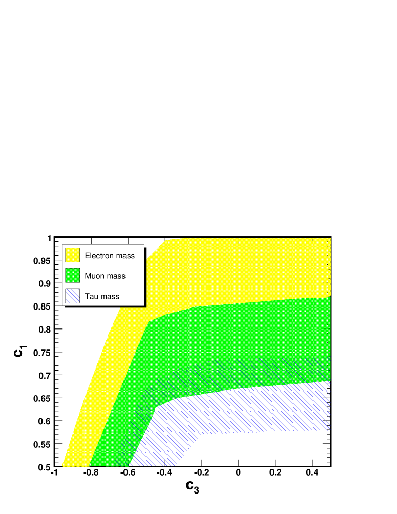
Figure 1: Region of $c_{1}$, $c_{3}$ parameter space consistent with the known charged lepton masses. The bands correspond to variations of the values of the $\tilde{k}$ and $M_{L_{2}}$ parameters in the range 1.5 TeV $\stackrel{{\scriptstyle<}}{{{}_{\sim}}}\tilde{k}\stackrel{{\scriptstyle<}}{{{}_{\sim}}}$ 5.5 TeV and $0.1\stackrel{{\scriptstyle<}}{{{}_{\sim}}}M_{L_{2}}\stackrel{{\scriptstyle<}}{{{}_{\sim}}}5$.

3.2 Neutrino Masses

The Neutrino masses are analyzed in a similar manner. First we look at the case in which the left-handed and right-handed neutrinos belong to the same muliplet case. For $c_{1}>0.5$,

$$\left(\frac{z}{\tilde{k}}\right)=\frac{(c_{1}-\frac{1}{2})e^{2(\frac{1}{2}-c_{1})kL}\sin[\frac{\lambda h}{f_{h}}]^{2}}{M_{IR}}$$ (110)

From Eq. (110) we see that values of $c_{1}\sim 1$ would be necessary in order to get the correct values for the neutrino masses. However, values of $c_{1}\simeq 1$ are strongly constrained in order to reproduce the proper charged lepton masses. Indeed, as we emphasized at the end of last section, the proper values of $\tau$ and $\mu$ masses may not be obtained for $c_{1}\sim 1$. Therefore, we conclude that if all $c_{1}$’s are about the same, as preferred to obtain large flavor mixing naturally without inducing large lepton flavor changing effects [36], two multiplets are required in order to obtain the correct lepton spectrum.

In the two multiplet case, the dependence of the neutrino masses on the mixing with the third multiplet through $M_{L_{2}}$ is always exponentially suppressed. Therefore, we shall set $M_{L_{2}}=0$ in the following approximate expressions. The approximate mass expressions, for

• $c_{1}>0.5$ and $c_{2}>1/(k\;L)$:

  $$\left(\frac{z}{\tilde{k}}\right)=\frac{M_{L_{1}}^{2}(c_{1}-\frac{1}{2})e^{2(\frac{1}{2}-c_{1})kL}\sin\left[\frac{\lambda h}{f_{h}}\right]^{2}}{M_{IR}}$$ (111)

• $c_{1}>0.5$ and $c_{2}<-1/(k\;L)$:

  $$\left(\frac{z}{\tilde{k}}\right)=\frac{M_{L_{1}}^{2}(c_{1}-\frac{1}{2})e^{2(\frac{1}{2}-c_{1}+c_{2})kL}\sin\left[\frac{\lambda h}{f_{h}}\right]^{2}}{M_{UV}}$$ (112)

• $c_{1}>0.5$ and $c_{2}\sim 0$:

  $$\left(\frac{z}{\tilde{k}}\right)=\frac{M_{L_{1}}^{2}(c_{1}-\frac{1}{2})e^{2(\frac{1}{2}-c_{1})kL}\sin\left[\frac{\lambda h}{f_{h}}\right]^{2}}{M_{UV}+M_{IR}}$$ (113)

where in Eq. (113) we have assumed $M_{UV}\neq-M_{IR}$.

In the linear regime, $(\lambda h/f_{h})^{2}\ll 1$, these neutrino masses become proportional to the square of the Higgs vev, and show the characteristic See-Saw behavior governed by the brane Majorana masses. From the above expressions we see that it will only be possible to generate the correct order of the neutrino masses when $c_{2}\stackrel{{\scriptstyle>}}{{{}_{\sim}}}-0.4$. Moreover, for $c_{2}\gtrsim 0$, the values of $c_{1}$ are such that the correct heavy lepton masses cannot be generated. These conclusions are verified in our numerical work. We present the relevant parameter space in the $c_{1}-c_{2}$ plane leading to the correct order of the neutrino masses in Fig. 2. The width of the bands for the different masses corresponds to varying $\tilde{k}$ and the different brane masses in the range indicated in Fig. 2. As indicated by the above expressions, we were not able to numerically find any solutions for $c_{2}<-0.5$. Finally, although positive values of $c_{2}$ are not represented in Fig. 2, the neutrino masses become independent of $c_{2}$ for $c_{2}>0$, and therefore the values of $c_{1}$ are the same as for $c_{2}=0$.

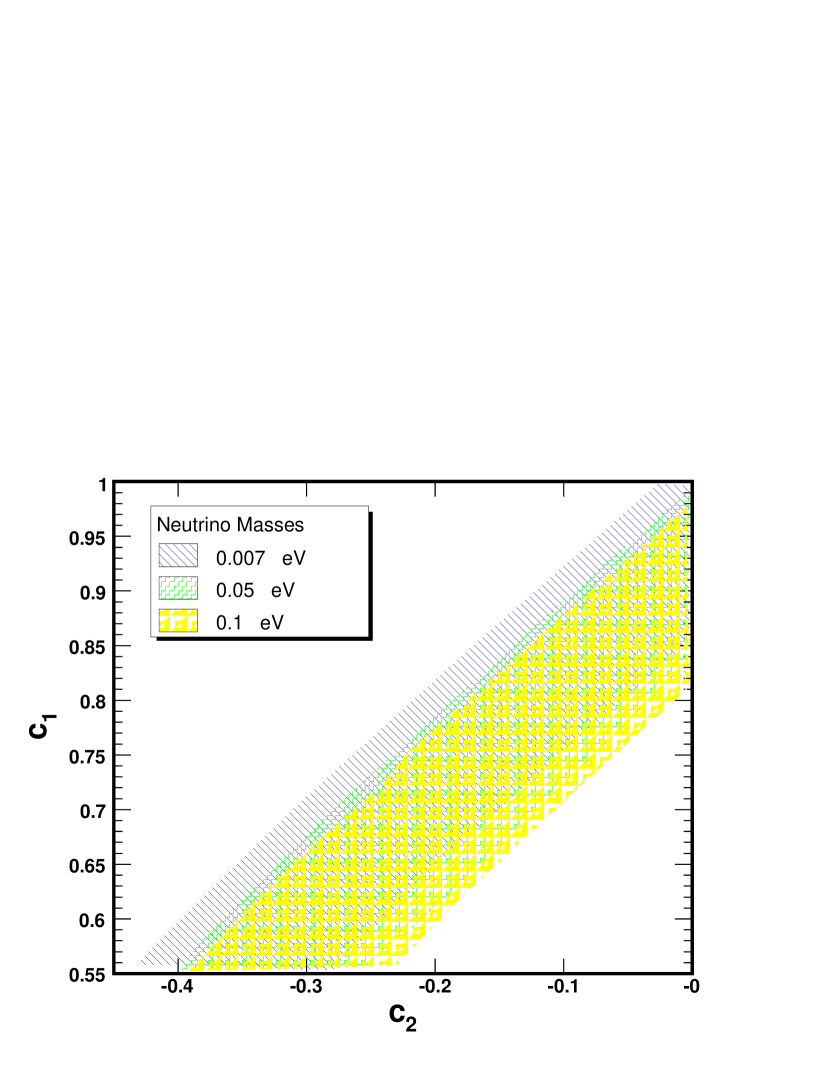
Figure 2: Region of $c_{1}$, $c_{2}$ parameter space consistent with the neutrino masses of interest: $c_{1}>0.5$ and $-0.5<c_{2}<0$. The bands correspond to variations of the values of the parameters $\tilde{k}$, $M_{L_{1}}$ and $M_{UV,IR}$ in the range 1.5 TeV $\stackrel{{\scriptstyle<}}{{{}_{\sim}}}\tilde{k}\stackrel{{\scriptstyle<}}{{{}_{\sim}}}$ 5 TeV, $0.1\stackrel{{\scriptstyle<}}{{{}_{\sim}}}M_{L_{1}}\stackrel{{\scriptstyle<}}{{{}_{\sim}}}1.5$ and $0.5\stackrel{{\scriptstyle<}}{{{}_{\sim}}}M_{IR,UV}\stackrel{{\scriptstyle<}}{{{}_{\sim}}}2.5$.

3.3 Flavor Problem

In the above, we have not discussed the problem of flavor. It is well known that, if the effective Yukawa couplings have an anarchic structure, large flavor violating effects are induced, which may only be suppressed by pushing the KK masses to values above 10 TeV, excluding any possible phenomenology of warped extra dimensional models at the LHC, as well as any possible dark matter candidate coming from the KK modes (see, for example Ref. [33] as well as Ref. [34] for an alternative approach to this question). The problem stems in part from the fact that the Yukawa couplings and the bulk mass parameters are not diagonalized in the same basis, and therefore the quark mass eigenstates have flavor violating couplings with the gluon KK modes. A possible solution to this problem is to demand an alignment between the bulk mass parameters and the Yukawa couplings, as has been proposed in Ref. [35]. Flavor violation in the lepton sector can also be suppressed by a similar alignment [36],[37]. This is equivalent to demanding that the bulk mass parameters obey the following relationships:

$$c_{3} = I+a_{3}k^{2}Y_{l}^{\dagger}Y_{l}$$

$$c_{2} = I+a_{2}k^{2}Y_{\nu}^{\dagger}Y_{\nu}$$

$$c_{1} = I+a_{l}k^{2}Y_{l}Y_{l}^{\dagger}+a_{\nu}k^{2}Y_{\nu}Y_{\nu}^{\dagger};$$ (114)

where $Y_{l}$ and $Y_{\nu}$ are the effective charged lepton and neutrino Yukawa couplings and $a_{l}$, $a_{\nu}$, $a_{2}$ and $a_{3}$ are numerical constants and the $c_{i}$ are now matrices where the off-diagonal terms mix the different generations.

The Gauge-Higgs unification structure introduced above demands a redefinition of the above equations, since no explicit Yukawa coupling has been written. As can be seen from Eqs. (107)–(109), and Eqs. (111)–(113), the role of the Yukawa coupling is now being played by the boundary masses $M_{L_{1}}$ and $M_{L_{2}}$. Hence, the above equations must be rewritten as

$$c_{3} = I+a_{32}M_{L_{2}}^{\dagger}M_{L_{2}}$$

$$c_{2} = I+a_{21}M_{L_{1}}^{\dagger}M_{L_{1}}$$

$$c_{1} = I+a_{12}M_{L_{2}}M_{L_{2}}^{\dagger}+a_{11}M_{L_{1}}M_{L_{1}}^{\dagger};$$ (115)

If $a_{12}\gg a_{11}$, the charged lepton masses would be diagonalized in the same basis as the bulk mass parameters, inducing minimal flavor violation in the lepton sector. In this case, all flavor violation will be associated with the charged currents, leading to values of the lepton flavor violation processes consistent with experiment for KK masses as low as a few TeV. As emphasized above, large mixing angles may naturally arise within this framework, if all left-handed zero modes localization parameters take equal values, namely when $a_{12}\simeq a_{11}\simeq 0$ [36].

The results of Refs. [36],[37] show that it is possible to impose a flavor symmetry in this class of models such that no large flavor violation occurs. In this work, we will assume that this, or a similar [38],[39],[40] flavor protection exists, and will postpone a more detailed analysis of this question for future work.

4 Dark Matter

Dark Matter in warped extra dimensions was first introduced in Ref. [41] within a framework which solves the proton stability problem in unification scenarios. The introduction of a KK parity in warped extra dimensions, leading to a stable dark matter candidate, was further proposed in Ref. [42]. In this work, we shall proceed in a different way: Following Ref. [43], we shall introduce an additional exchange $Z_{2}$ symmetry under which all the lepton multiplets introduced so far would be even. One can then define extra fermion multiplets, that will be chosen as the “odd” partners of the lepton multiplets. If this symmetry is preserved, the lightest odd particle (LOP) will be stable, and therefore can be considered as a possible dark matter candidate. In the framework of Ref. [43] the equality of the even and odd mass parameters was enforced by giving the original fermions, whose even and odd combinations form the even and odd fields, different charges under an extended $U(1)_{X_{1}}\times U(1)_{X_{2}}$ gauge symmetry. Since in our case the leptons are neutral under $U(1)_{X}$ this property does not hold. Additionally, contrary to Ref. [43], we shall assume that the quark and gauge boson multiplets do not have odd partners.

Even though, the structure of our model does not require the equality of the bulk masses for the odd and even fields, for simplicity, we shall assume that the bulk mass parameters are identified with each other and are controlled by the requirement of obtaining the correct small neutrino masses via the see-saw mechanism. Our assumption is equivalent to requiring that there are no off-diagonal bulk mass parameters mixing the original fields for which the $Z_{2}$ exchange symmetry holds.

In order to explore this possibility, we shall identify the multiplet containing the dark matter candidate with the odd partners of the second lepton multiplet containing the right-handed neutrinos. As has been shown in the previous section, this demands values of $c_{2}\stackrel{{\scriptstyle<}}{{{}_{\sim}}}0$, and therefore we shall require the bulk mass parameter of the dark matter candidate to be in this range.

The exchange symmetry, introduced in Ref. [43] allows arbitrary boundary masses between even fields, necessary for obtaining the proper lepton masses, as well as between the odd fields. Boundary masses mixing odd and even fields are, instead, forbidden by this symmetry. On the other hand, the boundary conditions for the even and odd fields are independent of each other. Therefore, the main link between even and odd fields is through the identification of the bulk mass parameters. For simplicity, we shall choose the boundary conditions of the odd partners of the chiral first and third lepton multiplets, containing the left-handed and right-handed charged leptons, to be the same as the one of the even biodoublet components, (- +) and (+ -), respectively. For values of the bulk masses $c_{1}>0.5$ and $c_{3}<-0.5$, these fields will be relatively heavy, with masses about a few times $\tilde{k}$, and decoupled from the Higgs.

For the second multiplet, the odd fields, denoted by $\xi_{o}$ will have the same boundary conditions as $\xi_{2}$ for the even bidoublets. However, since the fifth component does not contain a zero mode, it must have different boundary conditions on the IR and UV branes. That leaves us with two options for the left handed component of this field: $(+,-)$ or $(-,+)$. The goal here is to consider the possibility of a neutral odd lepton, mainly singlet under the $SU(2)_{L}\times SU(2)_{R}$ symmetry, as a dark matter candidate. The singlet and the doublet states mix via their interactions with the Higgs field, which will act as a small perturbation to their masses. In order to make the coupling to the Higgs effective and to split the doublet and singlet masses, we shall choose the singlet right-handed field to have the same boundary conditions on the IR brane as the bidoublet left-handed field for at least one of the three odd partners of the second multiplets. Therefore, the boundary conditions for the odd multiplet containing the LOP are chosen to be:

$$\begin{array}[]{c}\begin{array}[]{ccccccc}\xi^{o}_{R}&\sim&L^{o}_{R}&=&\begin{pmatrix}C^{o}_{R}(-,+)_{1}&n^{\prime{o}}_{R}(-,+)_{0}\\ n^{o}_{R}(-,+)_{0}&C^{\prime{o}}_{R}(-,+)_{-1}\end{pmatrix}&\oplus&N^{o}_{R}(+,-)_{0}\leavevmode\nobreak\ ,\end{array}\end{array}\vspace{3mm}$$ (118)

Regarding the other two generations of odd partners of the second multiplets, for simplicity, we will choose their singlet states to have the opposite boundary conditions from the one presented in Eq. (118). This would force their masses to be heavy for $c_{2}\leq 0$, ensuring that the multiplet with the boundary conditions given by Eq. (118), $\xi_{o}$, would generate the LOP. In addition, small Dirac boundary masses may be included, which would allow a small mixing between the odd multiplets inducing decays of the heavier generation odd states to the LOP, through the weak gauge bosons and the Higgs boson. Even in the case of a very small mixing, due to the large mass differences, the lifetime of these heavy odd partners would naturally be very short, and therefore these heavier odd multiplets would not contribute to the LOP relic density in any relevant way.

Finally, in order to estimate the dark matter density, we shall restrict ourselves to the first level of odd KK modes, since they give the dominant contribution to the annihilation cross section. This is due not only to their relatively small masses with respect to the heavier modes in the tower, but also due to their larger couplings to the LOP. We have checked that the inclusion of the second KK level leads to a very small modification of the annihilation cross section and therefore of the freeze-out temperature and the predicted relic density. Let us finally comment that in the region consistent with the proper dark matter density, the mixing between the singlet and doublet particles is small and these particles lead to only a small contribution to the Higgs effective potential and the precision electroweak observables.

Similar to the standard model fields discussed in the previous section, the boundary conditions, Eq. (118), lead to a set of equations which determine the masses of our odd multiplet fermions. For the KK modes that couple to the Higgs boson, in the case of vanishing Majorana masses for the odd fields, we find the following condition

$$\sin\left[\frac{\lambda h}{f_{h}}\right]^{2}+\dot{\tilde{S}}_{M_{2}}\dot{\tilde{S}}_{-M_{2}}=0.$$ (119)

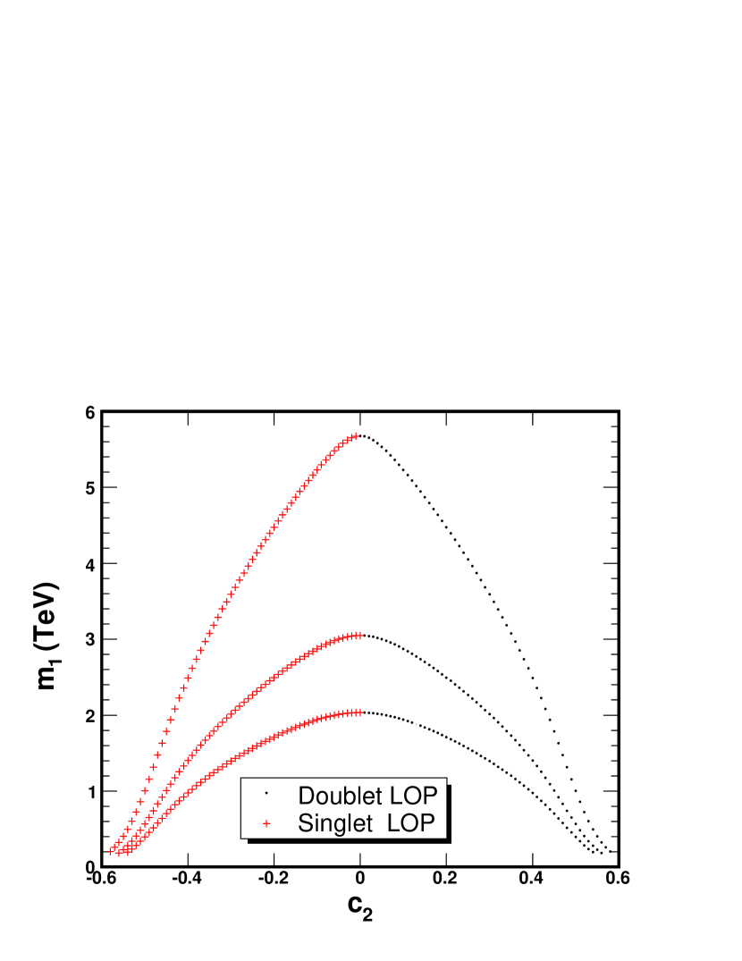
Figure 3: The Dirac mass of the LOP, $m_{1}$ as a function of $c_{2}$, the localization parameter for the odd fermions for three values of $\tilde{k}=\leavevmode\nobreak\ 1.5,\leavevmode\nobreak\ 2.2$ and $3.8$ TeV.

The solutions for the LOP are plotted in Fig. 3. The behavior of the LOP mass may be understood from the $h=0$ limit. In this limit, the singlet and doublet states don’t mix and the singlet becomes the lightest odd particle for $c_{2}<0$, while the doublet becomes the LOP for $c_{2}>0$. At $c_{2}=0$ and $h=0$, the singlet and doublet masses are degenerate. When $h\neq 0$ the singlet and doublet states mix and their masses are split by the Higgs v.e.v. Only the lightest state mass is plotted in Fig. 3. In the presence of the Higgs, at $c_{2}=0$, the LOP is an equal admixture of the singlet and doublet state. As we move away from $c_{2}=0$, the roots of the determinant will start splitting into two clearly spaced masses. For $c_{2}<0$, the lighter mass is mostly a singlet state and the heavier one is mostly a doublet state. Since these are Dirac particles, the positive and negative roots of the determinant are equal.

4.1 Odd Majorana Masses

In the above, we have not considered the impact of Majorana mass terms that could in principle be written for this multiplet, both on the IR and the UV branes, as was done for the even neutrinos, and would modify the couplings to the Higgs boson. Including the Majorana masses for the odd multiplet, the equation determining the odd lepton masses is given by

$$\dot{\tilde{S}}_{-M_{2}}\left(\dot{\tilde{S}}_{M_{2}}-M_{IR_{o}}\tilde{S}_{M_{2}}-e^{2c_{2}kL}M_{UV_{o}}\left(\tilde{S}_{-M_{2}}-M_{IR_{o}}\dot{\tilde{S}}_{-M_{2}}\right)\right)+\sin\left[\frac{\lambda h}{f_{h}}\right]^{2}=0$$

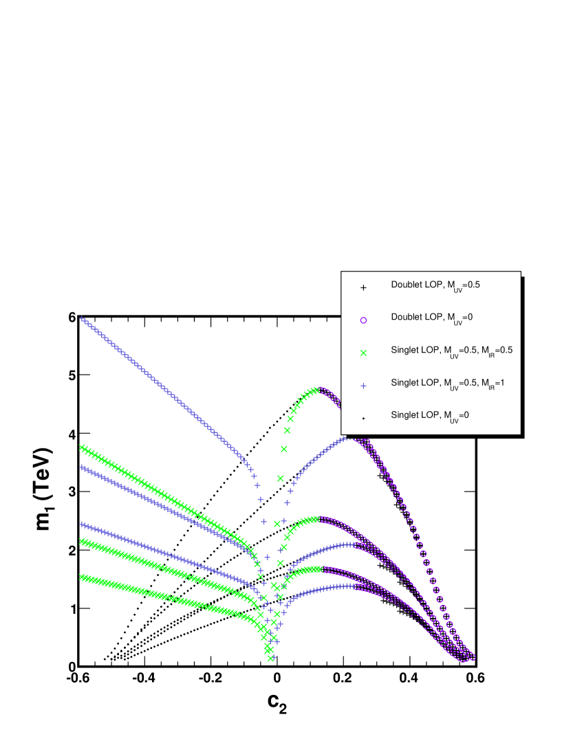
Figure 4: The Majorana mass of the LOP, $m_{1}$ as a function of $c_{2}$, the localization parameter for the odd fermions, with different values of $M_{UV}$ marked, and for three values of $\tilde{k}=\leavevmode\nobreak\ 1.5,\leavevmode\nobreak\ 2.2$ and $3.8$ TeV (corresponding to the three convergent purple circle lines from bottom to top for $c_{2}>0$), and two different values of $M_{IR_{o}}=\leavevmode\nobreak\ 1$ and $0.5$ for each $\tilde{k}$ and $M_{UV_{o}}$ (from top to bottom for $c_{2}<0$).

The effect of introducing the Majorana mass terms can be seen in the different negative and positive masses as one moves away from $M_{UV_{o}},M_{IR_{o}}=0$. Due to the different behavior of the functions $\tilde{S}$ and $\dot{\tilde{S}}$, by inspection, we can see that the positive and negative roots of Eq. (4.1) will no longer be equal. The two Dirac states have been split into four Majorana states. These states can still be recognized as two mostly singlet and two mostly doublet states by comparing their masses to the charged states. In the following, we will sometimes refer to these states as singlet or doublet, where it should be understood that these are not really the original states, but those mixed by the Higgs. Without the mixing, the coupling between the singlet-singlet and the doublet-doublet states and the Higgs would vanish. Therefore, we expect the singlet-singlet coupling to be suppressed compared with the coupling of the mostly singlet state to the mostly doublet states. Additionally, looking at Fig. 4 we see that as expected, the Majorana masses don’t effect the mass of the LOP when the LOP is mainly a doublet state (purple circles for $c_{2}>0$), as the convergence of the different curves corresponding to the different values of $M_{IR_{o}}$ and $M_{UV_{o}}$ clearly show.

The behavior of the LOP mass as well as its coupling to the Higgs may be studied by looking at the roots of Eq. (4.1). Using the small $z$ expansion for $\tilde{S}_{M}$, we obtain

$$z\sim 2\leavevmode\nobreak\ \tilde{k}\leavevmode\nobreak\ \left(\frac{1}{2}+c_{2}\right)\leavevmode\nobreak\ \frac{M_{IR_{o}}M_{UV_{o}}-e^{2c_{2}kL}\cos\left[\frac{\lambda h}{f_{h}}\right]^{2}}{e^{2c_{2}kL}M_{IR_{o}}+4\frac{(\frac{1}{2}+c_{2})}{(\frac{1}{2}-c_{2})}M_{UV_{o}}}\leavevmode\nobreak\ ,$$ (121)

which is valid for the case in which at least one of the Majorana masses is non-vanishing and $c_{2}<0$, in which the singlet becomes the LOP. This clearly shows that when only one of the Majorana masses is non-zero, we get a See-Saw effect governing the LOP mass. This behavior is confirmed in our numerical analysis plotted in Fig. 4.

Observe that if only the ultraviolet mass is non-vanishing, the mass of the LOP (which is mainly a left-handed singlet) is exponentially suppressed, unless $c_{2}\simeq 0$. Indeed, in the limit of vanishing infrared Majorana masses, Eq. (121) reduces to

$$z\sim\leavevmode\nobreak\ -\tilde{k}\leavevmode\nobreak\ \left(\frac{1}{2}-c_{2}\right)\leavevmode\nobreak\ \frac{e^{2c_{2}kL}\cos\left[\frac{\lambda h}{f_{h}}\right]^{2}}{2M_{UV_{o}}}\leavevmode\nobreak\ .$$ (122)

As can be seen from Eq. (122), the higher operator coupling of the LOP to the Higgs is also suppressed for $c_{2}<0$. We will show that the annihilation cross section for a mainly singlet state is sufficiently enhanced only when the s-channel Higgs diagram becomes sizable and therefore, unless $c_{2}\simeq 0$, the Dark Matter density becomes very large compared to the experimentally observed value.

As both $M_{IR_{o}}$ and $M_{UV_{o}}$ are turned on, we see an abrupt change in the behavior of the mass spectrum for $c_{2}<0$, which becomes independent of the exact value of $M_{UV_{o}}$ and only depends on $\tilde{k}$ and $M_{IR_{o}}$,

$$z\sim\leavevmode\nobreak\ \frac{\tilde{k}\;M_{IR_{o}}}{2}\leavevmode\nobreak\ \left(\frac{1}{2}-c_{2}\right)\leavevmode\nobreak\ .$$ (123)

The LOP mass in this case is of the order of $\tilde{k}$, and does not show an explicit dependence on the Higgs vaccum expectation value. Indeed, as can be seen from Eq. (121), the effective coupling to the Higgs for $c_{2}<0$ is exponentially suppressed. Therefore, as happens in the case of vanishing $M_{IR_{o}}$, a good dark matter candidate may only be obtained for values of $c_{2}\gtrsim 0$.

When $c_{2}\sim 0$, the mass can be approximated by:

$$z\sim\tilde{k}\frac{M_{IR_{o}}M_{UV_{o}}-e^{2c_{2}kL}\cos\left[\frac{\lambda h}{f_{h}}\right]^{2}}{e^{2c_{2}kL}M_{IR_{o}}+4M_{UV_{o}}}$$ (124)

We see that for $M_{IR_{o}},\leavevmode\nobreak\ M_{UV_{o}}\sim\mathcal{O}(1)$, for values of $h$ in the linear regime and very small values of $c_{2}$, we can get a cancelation resulting in very small LOP masses. This behavior is clearly portrayed in Fig. 4.

Finally, let us analyze the case $M_{IR_{o}}\neq 0$ and $M_{UV_{o}}=0$. As $M_{IR_{o}}$ is turned on, it strongly modifies the spectrum with respect to the Dirac case for negative values of $c_{2}$. In this case, the LOP becomes mostly a right-handed singlet and its mass is given by

$$z\sim\leavevmode\nobreak\ -\tilde{k}\leavevmode\nobreak\ (1+2c_{2})\leavevmode\nobreak\ \frac{\cos\left[\frac{\lambda h}{f_{h}}\right]^{2}}{M_{IR_{o}}}\leavevmode\nobreak\ .$$ (125)

As seen in Eq. (125), the LOP mass in this case is, again, of the order of the weak scale but with an explicit Higgs v.e.v. dependence induced by a higher order operator coupling with a characteristic scale of the order of the KK masses. Therefore the coupling of the LOP to the Higgs becomes sizable for KK masses of the order of the TeV scale, allowing for the possibility of a dark matter candidate for $c_{2}<0$.

In the following section, we shall perform a more precise quantitative analysis of the masses and couplings associated with the annihilation cross section of the singlet state for both the Majorana and Dirac cases.

4.2 Couplings of the Odd Leptons

4.2.1 Higgs Couplings

To calculate the couplings of the Majorana and Dirac states with the Higgs, the profile function of the odd leptons which couple to the Higgs bosons need to be computed. The mass eigenstate profile functions are given in terms of combinations of the profile functions without the Higgs. In the particular case of the neutral odd leptons these are admixtures of the neutral states belonging to the bidoublet and the singlet state, with normalization coefficients $C_{2}$, $C_{3}$ and $C_{5}$.

The boundary conditions determine the coefficients $C_{3}$ and $C_{5}$ as functions of $C_{2}$. The fermion profile functions in the presence of the Higgs are given by:

$$f_{L}^{2}(h) = \frac{1}{2}e^{\frac{1}{2}(1-2c_{2})kx}\left(e^{2c_{2}kx}\dot{\tilde{S}}_{-M_{2}}\left(C_{2}\left(1+\cos\left[\frac{\lambda h}{f_{h}}\right]\right)-C_{3}\left(1-\cos\left[\frac{\lambda h}{f_{h}}\right]\right)\right)\right.$$ (126)

$$-\left.\sqrt{2}(\tilde{S}_{M_{2}}-e^{2c_{2}kx}M_{UV_{o}}\dot{\tilde{S}}_{-M_{2}})\leavevmode\nobreak\ C_{5}\sin\left[\frac{\lambda h}{f_{h}}\right]\right)$$

$$f_{L}^{3}(h) = \frac{1}{2}e^{\frac{1}{2}(1-2c_{2})kx}\left(e^{2c_{2}kx}\dot{\tilde{S}}_{-M_{2}}\left(C_{3}\left(1+\cos\left[\frac{\lambda h}{f_{h}}\right]\right)-C_{2}\left(1-\cos\left[\frac{\lambda h}{f_{h}}\right]\right)\right)\right.$$ (127)

$$-\left.\sqrt{2}(\tilde{S}_{M_{2}}-e^{2c_{2}kx}M_{UV_{o}}\dot{\tilde{S}}_{-M_{2}})\leavevmode\nobreak\ C_{5}\sin\left[\frac{\lambda h}{f_{h}}\right]\right)$$

$$f_{L}^{5}(h) = \frac{1}{2}e^{\frac{1}{2}(1-2c_{2})kx}\left(2(\tilde{S}_{M_{2}}-e^{2c_{2}kx}M_{UV_{o}}\dot{\tilde{S}}_{-M_{2}})\leavevmode\nobreak\ C_{5}\cos\left[\frac{\lambda h}{f_{h}}\right]+\sqrt{2}e^{2c_{2}kx}\dot{\tilde{S}}_{-M_{2}}(C_{2}+C_{3})\sin\left[\frac{\lambda h}{f_{h}}\right]\right)$$

$$f_{R}^{2}(h) = \frac{1}{2}e^{\frac{1}{2}(1-2c_{2})kx}\left(e^{2c_{2}kx}\tilde{S}_{-M_{2}}\left(C_{2}\left(1+\cos\left[\frac{\lambda h}{f_{h}}\right]\right)-C_{3}\left(1-\cos\left[\frac{\lambda h}{f_{h}}\right]\right)\right)\right.$$ (129)

$$+\left.\sqrt{2}(e^{2c_{2}kx}M_{UV_{o}}\tilde{S}_{-M_{2}}-\dot{\tilde{S}}_{M_{2}})\leavevmode\nobreak\ C_{5}\sin\left[\frac{\lambda h}{f_{h}}\right]\right)$$

$$f_{R}^{3}(h) = \frac{1}{2}e^{\frac{1}{2}(1-2c_{2})kx}\left(e^{2c_{2}kx}\tilde{S}_{-M_{2}}\left(C_{3}\left(1+\cos\left[\frac{\lambda h}{f_{h}}\right]\right)-C_{2}\left(1-\cos\left[\frac{\lambda h}{f_{h}}\right]\right)\right)\right.$$ (130)

$$+\left.\sqrt{2}(e^{2c_{2}kx}M_{UV_{o}}\tilde{S}_{-M_{2}}-\dot{\tilde{S}}_{M_{2}})\leavevmode\nobreak\ C_{5}\sin\left[\frac{\lambda h}{f_{h}}\right]\right)$$

$$f_{R}^{5}(h) = \frac{1}{2}e^{\frac{1}{2}(1-2c_{2})kx}\left(2(\dot{\tilde{S}}_{M_{2}}-e^{2c_{2}kx}M_{UV_{o}}\tilde{S}_{-M_{2}})\leavevmode\nobreak\ C_{5}\cos\left[\frac{\lambda h}{f_{h}}\right]+\sqrt{2}e^{2c_{2}kx}\tilde{S}_{-M_{2}}(C_{2}+C_{3})\sin\left[\frac{\lambda h}{f_{h}}\right]\right)$$

where the functions $\tilde{S}$ and $\dot{\tilde{S}}$ are functions of $x_{5}$ and the masses $z$ of the odd fermions.

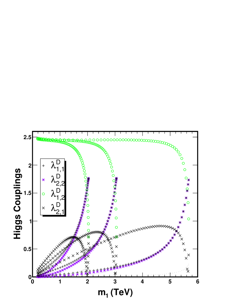
Figure 5: Higgs couplings to the Dirac particles for three values of $\tilde{k}\sim\leavevmode\nobreak\ 1.5,\leavevmode\nobreak\ 2.2$ and $3.8$ TeV corresponding to $m_{1}\sim\leavevmode\nobreak\ 2,\leavevmode\nobreak\ 3$ and $6$ TeV for $c_{2}=0$ from left to right, as a function of the singlet LOP mass $m_{1}$.

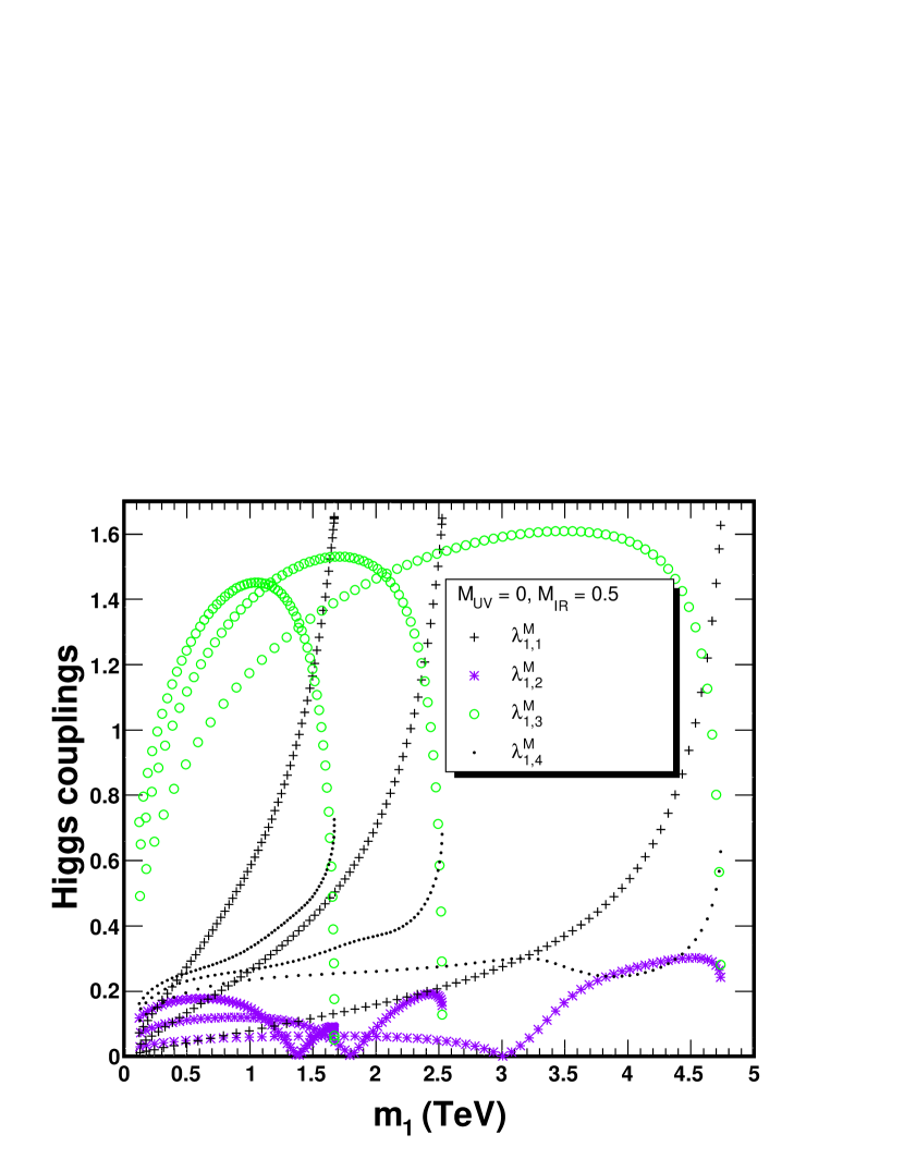
Figure 6: Higgs couplings to the Majorana particles for three values of $\tilde{k}\sim\leavevmode\nobreak\ 1.5,\leavevmode\nobreak\ 2.2$ and $3.8$ TeV corresponding to $m_{1}\sim\leavevmode\nobreak\ 1.7,\leavevmode\nobreak\ 2.5$ and $4.7$ TeV for $c_{2}=0$, from left to right, as a function of the singlet LOP mass $m_{1}$.

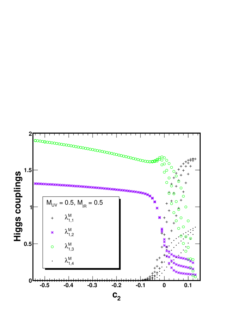
Figure 7: Higgs couplings to the Majorana particles for three values of $\tilde{k}\sim\leavevmode\nobreak\ 1.5,\leavevmode\nobreak\ 2.2$ and $3.8$ TeV as a function of $c_{2}$, when the singlet is the LOP. The smaller values of $\tilde{k}$ correspond to the smaller couplings (the lower curve).

For the doublet and singlet states mixed by the Higgs, a non-trivial solution may be only obtained if the following relations are fulfilled.

$$C_{3} = C_{2}$$ (132)

$$C_{5} = C_{2}\frac{\sqrt{2}e^{2c_{2}kL}\dot{\tilde{S}}_{-M_{2}}\cot\left[\frac{\lambda h}{f_{h}}\right]_{L}}{\tilde{S}_{M_{2}}-e^{2c_{2}kL}M_{UV_{o}}\dot{\tilde{S}}_{-M_{2}}};.$$ (133)

For the neutral leptons which decouple from the Higgs, instead, the following relations are fulfilled:

$$C_{3} = -C_{2}$$ (134)

$$C_{5} = 0$$ (135)

This implies that only the symmetric combination of neutral bidoublet states with coefficients given by Eq. (132) and (133), couple to the Higgs. Moreover, the normalization coefficient $C_{2}$ may be computed by demanding well normalized functions, namely,

$$C_{2}=\left(\int^{L}_{0}\frac{\sum_{i=2,3,5}\left(|f_{L}^{i}|^{2}+|f_{R}^{i}|^{2}\right)}{|C_{2}|^{2}}dx\right)^{-1/2}.$$ (136)

The above definition is appropriate in the Majorana case, in which the left-handed components of the fermions acquire contributions from both the original left-handed and the (charge conjugate) right-handed modes, Eqs. (126)–(LABEL:fr5). In the Dirac case, the left-handed and right-handed functions acquire equal normalizations and therefore the proper factor $C_{2}$ is equal to the one computed above divided by $\sqrt{2}$. In the following, we will keep the above definition of $C_{2}$ for both the Majorana and Dirac cases and take care of the proper $\sqrt{2}$ factors explicitly.

To calculate the couplings, we also need the Higgs profile and normalization:

$$f_{h} = C_{h}e^{2kx}$$ (137)

$$C_{h} = \frac{g_{5}}{\sqrt{\int_{0}^{L}a(x)^{-2}dx}}$$ (138)

Defining $\Xi(m_{i},m_{j})$:

$$\Xi(m_{i},m_{j})=-\frac{e^{-kx}}{2}C_{h}C_{2}^{*}(m_{i})C_{2}(m_{j})f_{h}\left[f_{R}^{5*}(m_{i})\left[f_{L}^{2}(m_{j})+f_{L}^{3}(m_{j})\right]-\left[f_{R}^{2*}(m_{i})+f_{R}^{3*}(m_{i})\right]f_{L}^{5}(m_{j})\right]$$ (139)

the left-right couplings of the Higgs with the different states, $\bar{\Psi}^{i}_{L}H\Psi^{j}$, in the Majorana and Dirac cases can be written as:

$$\lambda^{M}_{i,j} = \int^{L}_{0}\left(\Xi(m_{i},m_{j})+\Xi^{*}(m_{j},m_{i})\right)\leavevmode\nobreak\ dx$$ (140)

$$\lambda^{D}_{i,j} = 2\int^{L}_{0}\Xi(m_{i},m_{j})\leavevmode\nobreak\ dx$$ (141)

the factor of $2$ in the Dirac coupling is due to the definition of the $C_{2}$ factor discussed above. Observe that, while in the Majorana case $\lambda^{M}_{ij}=\lambda^{M\;*}_{ji}$, there is no such relation in the Dirac case.

The different couplings are plotted in Figs. 5 – 7. For the Dirac case and $c_{2}\stackrel{{\scriptstyle<}}{{{}_{\sim}}}0$, represented in Fig. 5, small values of the masses are obtained for smaller values of $c_{2}$. The left-right couplings of the singlet and doublet states, $\lambda^{D}_{1,2}$ acquire large values for negative values of $c_{2}$. This stems from the fact that for this case, the left-handed singlet component is localized towards the IR brane. As $c_{2}$ goes to 0, the localization effects become less pronounced and this coupling starts getting suppressed. The $\lambda^{D}_{i,i}$ couplings have the opposite behavior to the cross couplings. For $c_{2}$ negative, the mass difference between the singlet and the doublet state is large, while their mixing is small. Since the self-couplings of the mass eigenstates are induced by the product of the singlet and doublet components of these states, they become very suppressed. However, as $c_{2}$ goes to zero, the mass eigenvalues become symmetric and antisymmetric combinations of the singlet and doublet states, and the self couplings of the mass eigenstates become large, while the cross couplings tend to zero.

In the Majorana case with $M_{UV_{o}}=0$, although the quantitative values are not the same, the $\lambda^{M}_{1,1}$ and $\lambda^{M}_{1,4}$ couplings behave similarly to the $\lambda^{D}_{1,1}$ couplings, since $m_{1}$ and $m_{4}$ are the two mostly singlet states, which are split due to the non-zero $M_{IR_{o}}$. When both the Majorana masses are non-zero, we see an abrupt change in the behavior of the couplings. As mentioned before, for $c_{2}<0$ the self-coupling of the lightest state is exponentially suppressed. This behavior is clearly demonstrated in the Higgs dependent part of the approximation for the LOP given in Eq. (121). The couplings of the LOP to the mostly doublet states, however, continue to be large.

4.2.2 Couplings to the $Z$ and $W^{\pm}$ Bosons

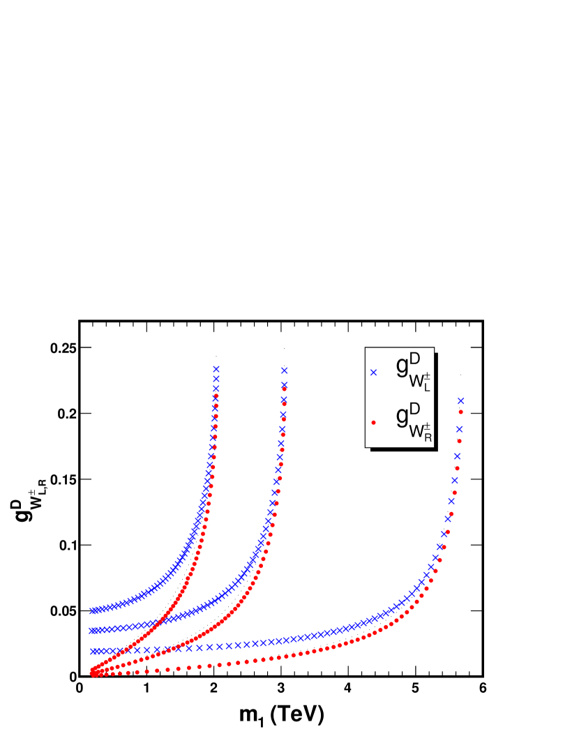
Figure 8: $W^{\pm}$ couplings to the Dirac particles for $c_{2}<0$ and three values of $\tilde{k}\sim\leavevmode\nobreak\ 1.5,\leavevmode\nobreak\ 2.2$ and $3.8$ TeV, which, for $c_{2}=0$, correspond approximately to $m_{1}\sim\leavevmode\nobreak\ 2,\leavevmode\nobreak\ 3$ and $5.6$ TeV, from left to right as a function of the singlet LOP mass. Larger values of $m_{1}$ are associated with larger values of $c_{2}$.

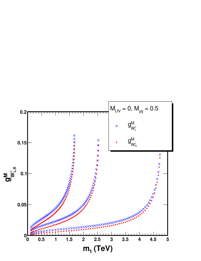
Figure 9: $W^{\pm}$ couplings of the Majorana particles for $c_{2}<0$ and three values of $\tilde{k}\sim\leavevmode\nobreak\ 1.5,\leavevmode\nobreak\ 2.2$ and $3.8$ TeV, which, for $c_{2}=0$. correspond to $m_{1}\sim\leavevmode\nobreak\ 1.7,\leavevmode\nobreak\ 2.5$ and $4.7$ TeV from left to right as a function of the singlet LOP mass. Larger values of $m_{1}$ are associated with larger values of $c_{2}$.

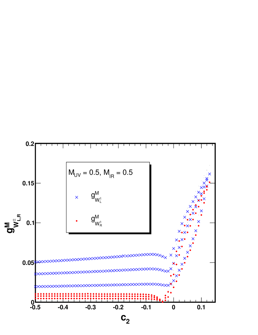
Figure 10: $W^{\pm}$ couplings to the Majorana particles for three values of $\tilde{k}\sim\leavevmode\nobreak\ 1.5,\leavevmode\nobreak\ 2.2$ and $3.8$ TeV as a function of $c_{2}$ for the singlet LOP. The smaller values of $\tilde{k}$ correspond to the smaller couplings (the lower curve).

The $Z$ couplings to the lepton sector are defined in a similar manner to the couplings with the quark sector [25],[26]. However, in the lepton case $Q_{X}=0$ and the neutral states that couple to the Higgs have $C_{3}=C_{2}$, implying that $f^{2}_{L,R}(h)=f^{3}_{L,R}(h)$. Therefore, the $Z$, and all its KK modes, as well as the neutral components of the $SU(2)_{R}$ gauge bosons don’t have any couplings with any two of these states. However, the orthogonal neutral state in the bidoublet, which does not couple to the Higgs has $C_{3}=-C_{2}$ and $C_{5}=0$. Hence, an off-diagonal coupling exists between this mode, the neutral states that couple to the Higgs and the $Z$.

The $W^{\pm}$ couple the charged fermions with the neutral components. In component form, the coupling is between $f^{1,4}_{L,R}(h)$ and $f^{2,3,5}_{L,R}(h)$. The profile functions and their normalization coefficients for the neutral components were given in Eqs. (LABEL:fr5) – (132). The charged fermions and the neutral component of the bidoublet which don’t couple to the Higgs state are both governed by the same five dimensional wave-function, namely:

$$f^{i}_{L} = C_{i}e^{\frac{1}{2}(1+2c_{2})kx}\dot{\tilde{S}}_{-M_{2}}$$ (142)

$$f^{i}_{R} = C_{i}e^{\frac{1}{2}(1+2c_{2})kx}\tilde{S}_{-M_{2}}$$ (143)

These fermion masses are given by the roots of $\tilde{\dot{S}}_{-M_{2}}$ and since the Majorana masses don’t influence them, they are always Dirac states. Further, it can be shown trivially that the $W^{-}$ coupling to the LOP and the positive charged state is equal to the coupling of the LOP to $W^{+}$ and the negative charged states. In the annihilation cross-section, we will only be interested in the couplings between the two charged fermions and the LOP. We will denote these couplings by $g_{W_{L,R}}$. The expression for these couplings is given in Appendix B. Similarly, for the $Z$ we will only be interested in the couplings between the LOP and the $N^{\prime}$ state, the neutral bidoublet component that does not mix with the Higgs, and we will denote these couplings by $g_{Z_{L,R}}$.

The gauge boson couplings are plotted in Figs. 8 – 10. Again we see that the Dirac and the Majorana, $M_{UV_{o}}=0$ couplings behave in a similar way. The coupling of the mostly singlet state to the charged or neutral fermion is obtained through the mixing with the bidoublet states. As discussed before, this mixing is small, for $c_{2}<0$, and increases for larger values of $c_{2}$. As $c_{2}$ approaches 0, in the Dirac case, we expect that since the mixing is maximal, the $W^{\pm}$ couplings should approach the neutrino-lepton SM coupling, $g_{w}/\sqrt{2}$, reduced by a factor $1/\sqrt{2}$, due to the mixing of the singlet with the doublet state, times another factor $1/\sqrt{2}$ due to the projection of the neutral doublet state on the $SU(2)$ partner of each of the charged fields. This behavior is clearly seen in Fig. 8, where only values of $c_{2}<0$ are plotted and increasing values of $m_{1}$ are associated with larger values of $c_{2}$. For $c_{2}<0$, the left-handed states which are located towards the infrared brane couple more strongly to the charged states than the right-handed states. Moreover, the couplings of the $Z$ and the $W^{\pm}$ become proportional to each other, with a coefficient of proportionality governed by $\cos\theta_{W}$, namely

$$g_{Z_{L,R}}=\frac{g_{W_{L,R}}}{\cos\theta_{W}}$$ (144)

The additional factor of $\sqrt{2}$ that appears between SM couplings of neutrinos to the $Z$ and $W$, is not present in this case.

In the case of zero ultraviolet Majorana mass but non-vanishing $M_{IR_{o}}$, depicted in Fig. 9, the behavior is similar to the Dirac case but the couplings are reduced due to the larger singlet components of the Majorana particles. Also, there is a sizable reduction of the left-handed couplings due to the larger right-handed component of the Majorana state. Observe that as $M_{UV_{o}}$ is turned on, for $c_{2}<0$, the couplings to the gauge bosons become independent of $c_{2}$.

Finally, as $c_{2}$ becomes positive, the couplings increase, due to the larger bidoublet component of the LOP.

4.3 Annihilation Cross Section

We will denote the neutral states mixed by the Higgs by $N_{i}$, where $i=1,2$, or $i=1,2,3,4$ for the two Dirac or four Majorana states respectively, where $i$ labels the states in increasing order of their absolute masses. $C^{\pm}$ will denote the charged fermions and, as said before, $N^{\prime}$ will denote the bidoublet neutral fermion which does not couple to the Higgs. The $N_{1}$ is the LOP, our dark matter candidate.

Ignoring co-annihilation effects, we consider the following five dominant processes for $N_{1}N_{1}$ annihilation: $N_{1}+\bar{N}_{1}\rightarrow t\leavevmode\nobreak\ \bar{t},\leavevmode\nobreak\ H\leavevmode\nobreak\ H,\leavevmode\nobreak\ Z\leavevmode\nobreak\ Z$ and $W^{+}\leavevmode\nobreak\ W^{-}$ (observe that due to the cancelation of the Z coupling to the states that couple to the Higgs, the $Z\leavevmode\nobreak\ H$ annihilation channel is suppressed). The Feynman diagrams contributing to each of these processes are shown in Figs. 11 – 14. The virtual $N_{i}$ exchanges in these diagrams should be understood to be summed over $i$, where $i$ as noted above runs over the appropriate index depending on whether we are considering the Dirac or the Majorana case. The $v$ in the following formulae is the relative velocity between the initial particles in the center of mass frame. $\lambda_{Htt}$, $\lambda_{HZZ}$, $\lambda_{HWW}$ and $\lambda_{H}$ are the couplings of the Higgs to the top, the $W^{\pm}$ and $Z$ bosons, and itself, which were discussed in Refs. [25] and [26].

4.3.1 $N_{1}+\bar{N}_{1}\rightarrow t+\bar{t}$

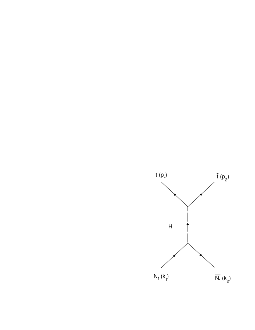
Figure 11: Feynman Diagram for the process $N_{1}+\bar{N}_{1}\rightarrow t+\bar{t}$

Due to the cancelation of the coupling of $N_{1}$ to the $Z$, the annihilation into fermion pairs proceeds via an s-channel Higgs interchange, and is therefore proportional to the corresponding fermion mass. Therefore, only the top contributes in a relevant way. The Dirac and Majorana cross-sections are given by the same formula, but the Higgs coupling should be understood to be the one appropriate for each case. Assuming $m_{1}>m_{t}$, we obtain:

$$<\sigma v>_{tt}=\frac{\lambda_{1,1}^{2}\lambda^{2}_{Htt}v^{2}}{8\pi m_{1}^{2}}\left(1-\frac{m_{t}^{2}}{m_{1}^{2}}\right)^{3/2}\left(1-\frac{m_{H}^{2}}{4m_{1}^{2}}\right)^{-2}$$ (145)

4.3.2 $N_{1}+\bar{N}_{1}\rightarrow H+H$

Figure 12: Feynman Diagrams contributing to the process $N_{1}+\bar{N}_{1}\rightarrow H+H$

The annihilation into Higgs pairs proceeds via an s-channel Higgs interchange diagram, which is subdominant, and the t-channel interchange of the neutral odd fermions. The result, in the limit $m_{H}\ll m_{1},m_{2}$, is given by:

$$<\sigma v>^{D}_{HH}=$$

$$\frac{v^{2}}{8\pi^{2}}\left[\frac{\lambda^{D\leavevmode\nobreak\ 2}_{1,1}}{16m_{1}^{2}}\frac{\lambda^{2}_{H}}{m_{1}^{2}}\right.$$

$$-\sum_{i}\frac{\lambda^{D}_{1,1}}{4m_{1}^{2}}\frac{\lambda_{H}}{m_{i}}\left(\left(\lambda^{D\leavevmode\nobreak\ 2}_{1,i}+\lambda^{D\leavevmode\nobreak\ 2}_{i,1}\right)\frac{m_{1}}{m_{i}}\left(1+\frac{m_{1}^{2}}{3m_{i}^{2}}\right)+2\lambda^{D}_{1,i}\lambda^{D}_{i,1}\left(1+\frac{m_{1}^{2}}{m_{i}^{2}}\right)\right)$$

$$+\sum_{i,j}\frac{1}{m_{i}m_{j}}\left(1+\frac{m_{1}}{m_{i}}\right)^{-2}\left(1+\frac{m_{1}}{m_{j}}\right)^{-2}\left(2\lambda^{D}_{1,j}\lambda^{D}_{j,1}\left(1+\frac{m_{1}^{2}}{m_{j}^{2}}\right)\left(2\lambda^{D}_{1,i}\lambda^{D}_{i,1}\left(1+\frac{m_{1}^{2}}{m_{i}^{2}}\right)\right.\right.$$

$$+\left.\left(\lambda^{D\leavevmode\nobreak\ 2}_{1,i}+\lambda^{D\leavevmode\nobreak\ 2}_{i,1}\right)\frac{m_{1}}{m_{i}}\left(1+\frac{m_{1}}{3m_{i}^{2}}\right)\right)+\left(\lambda^{D\leavevmode\nobreak\ 2}_{1,j}+\lambda^{D\leavevmode\nobreak\ 2}_{j,1}\right)\frac{m_{1}}{m_{j}}\left(\left(\lambda^{D\leavevmode\nobreak\ 2}_{1,i}+\lambda^{D\leavevmode\nobreak\ 2}_{i,1}\right)\frac{m_{1}}{m_{i}}\left(1+\frac{m_{1}}{3m_{i}^{2}}\left(1+\frac{m_{i}^{2}}{m_{j}^{2}}\right)\right.\right.$$

$$+\left.\left.\left.\frac{m_{1}^{4}}{m_{i}^{2}m_{j}^{2}}\right)+2\lambda^{D}_{1,i}\lambda^{D}_{i,1}\left(1+\frac{m_{1}^{2}}{m_{i}^{2}}\right)\left(1+\frac{m_{1}^{2}}{3m_{j}^{2}}\right)\right)\right]$$ (146)

where we have taken the couplings to be real. The sum runs over the two Dirac states labeled by their masses, $m_{1}$ and $m_{2}$. In the case of real couplings, the Majorana cross-section can be simply seen from the above with the replacement $\lambda^{M}_{i,j}=1/2(\lambda^{D}_{i,j}+\lambda^{D}_{j,i})$, and the indices now run over the four Majorana states:

$$<\sigma v>^{M}_{HH}=$$

$$\frac{v^{2}}{2\pi^{2}}\left[\frac{\lambda^{M\leavevmode\nobreak\ 2}_{1,1}}{64m_{1}^{2}}\frac{\lambda^{2}_{H}}{m_{1}^{2}}\right.$$

$$-\sum_{i}\frac{\lambda^{M}_{1,1}\lambda^{M\leavevmode\nobreak\ 2}_{1,i}}{8m_{1}^{2}}\frac{\lambda_{H}}{m_{i}}\left(\left(1+\frac{m^{2}_{1}}{m^{2}_{i}}\right)+\frac{m_{1}}{m_{i}}\left(1+\frac{m^{2}_{1}}{3m_{i}^{2}}\right)\right)$$

$$+\sum_{i,j}\frac{\lambda^{M\leavevmode\nobreak\ 2}_{1,j}\lambda^{M\leavevmode\nobreak\ 2}_{1,i}}{m_{i}m_{j}}\left(1+\frac{m_{1}}{m_{i}}\right)^{-2}\left(1+\frac{m_{1}}{m_{j}}\right)^{-2}\left(\left(1+\frac{m_{1}^{2}}{m_{j}^{2}}\right)\left(\left(1+\frac{m_{1}^{2}}{m_{i}^{2}}\right)+\frac{m_{1}}{m_{i}}\left(1+\frac{m^{2}_{1}}{3m^{2}_{i}}\right)\right)\right.$$

$$\left.+\frac{m_{1}}{m_{j}}\left(\frac{m_{1}}{m_{i}}\left(1+\frac{m_{1}}{3m_{i}^{2}}\left(1+\frac{m_{i}^{2}}{m_{j}^{2}}\right)+\frac{m_{1}^{4}}{m_{i}^{2}m_{j}^{2}}\right)+\left(1+\frac{m_{1}^{2}}{m_{i}^{2}}\right)\left(1+\frac{m_{1}^{2}}{3m_{j}^{2}}\right)\right)\right]$$ (147)

4.3.3 $N_{1}+\bar{N}_{1}\rightarrow W^{+}W^{-}$, $Z+Z$

The annihilation into the $W^{\pm}$ and $Z$ gauge bosons also proceeds via the s-channel interchange of a Higgs, plus the t-channel interchange of the charged fermion $C^{\pm}$ and the neutral fermion $N^{\prime}$, respectively. In the formula below, the label $G$ corresponds to either the $W^{\pm}$ or $Z$ gauge bosons, and $\alpha=1$ for the $W^{+}W^{-}$ cross-section and $\alpha=1/2$ for the $ZZ$ case. The diagrams contributing to the process in the Dirac case are given in Fig. 13. For the Majorana case, two additional diagrams contribute, and are given in Fig. 14. Using the properties of the Majorana couplings, one can demonstrate that these new diagrams are equal to the ones associated to the cross diagrams in the amplitudes for the annihilation into the $W^{\pm}$ (due to the interchange of the fermion of opposite charge) and $Z$ gauge bosons. Therefore, the cross-section is given by the same formula for both the Dirac and Majorana cases, but with appropriate couplings, and a factor $\beta=2$ for the Majorana case, and $\beta=1$ for the Dirac case. Although in the numerical analysis the full annihilation cross section was used, for simplicity, we will only quote the cross-section for the longitudinal modes, in the limit $m_{W},m_{Z}<m_{H}<<m_{1}$:

$$<\sigma v>_{GG} = \alpha\left[\frac{1}{4\pi m_{G}^{2}}\frac{m_{1}^{4}}{m_{f}^{4}}\left(g_{G_{L}}^{2}-g_{G_{R}}^{2}\right)^{2}\left(1+\frac{m_{1}^{2}}{m_{f}^{2}}\right)^{-2}\right.$$ (148)

$$+\leavevmode\nobreak\ \frac{m_{1}^{2}v^{2}}{\pi m_{G}^{4}}\left[\frac{\lambda^{2}_{1,1}}{16}\frac{\lambda_{HGG}^{2}}{m_{1}^{2}}\right.$$

$$-\leavevmode\nobreak\ \beta\leavevmode\nobreak\ \lambda_{1,1}\frac{\lambda_{HGG}}{m_{f}}\left(1+\frac{m_{1}^{2}}{m_{f}^{2}}\right)^{-2}\left(g_{G_{L}}g_{G_{R}}\left(1+\frac{m_{1}^{2}}{3m_{f}^{2}}\right)-\left(g^{2}_{G_{L}}+g^{2}_{G_{R}}\right)\frac{m_{1}}{3m_{f}}\left(1+\frac{m_{1}^{2}}{m_{f}^{2}}\right)\right)$$

$$+\leavevmode\nobreak\ \beta^{2}\leavevmode\nobreak\ \frac{2}{3}\frac{m_{1}^{2}}{m_{f}^{2}}\left(1+\frac{m_{1}^{2}}{m_{f}^{2}}\right)^{-4}\left(6g^{2}_{G_{L}}g^{2}_{G_{R}}\left(1+\frac{m_{1}^{2}}{m_{f}^{2}}+\frac{5m_{1}^{4}}{3m_{f}^{4}}+\frac{1}{3}\frac{m_{1}^{6}}{m_{f}^{6}}\right)-\frac{m_{1}}{m_{f}}\left(1+\frac{m_{1}^{2}}{m_{f}^{2}}\right)^{2}\right.$$

$$\qquad\left.\left.\left.\times\left(4g_{G_{L}}g_{G_{R}}\left(g^{2}_{G_{L}}+g^{2}_{G_{R}}\right)-\left(g^{4}_{G_{L}}+g^{4}_{G_{R}}\right)\frac{m_{1}}{m_{f}}\right)\right)\right]\right]$$

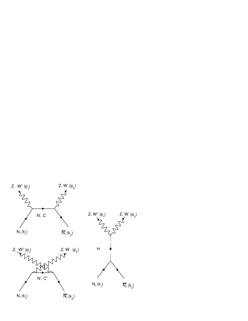
Figure 13: Feynman Diagrams contributing to the process $N_{1}+\bar{N}_{1}\rightarrow W^{+}W^{-},Z+Z$. The intermediate state is either the charged fermion $C^{\pm}$ for the $W^{\pm}$ case, or the orthogonal bidoublet, $N^{\prime}$ for the $Z$.

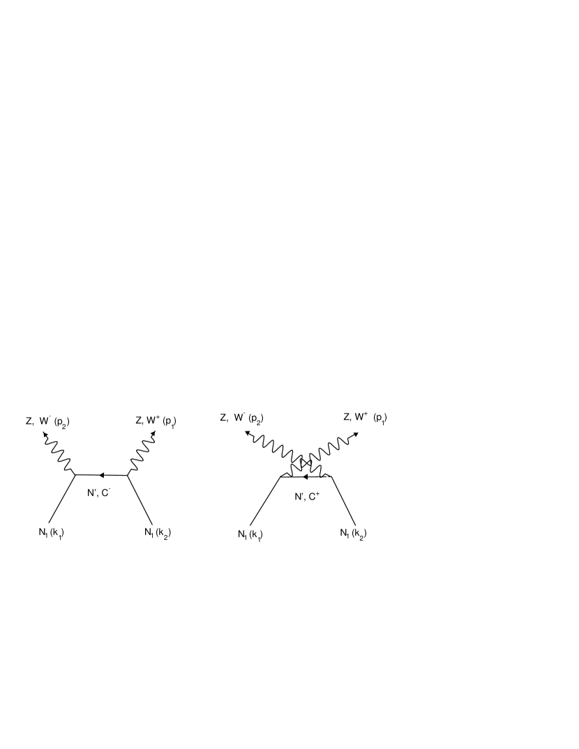
Figure 14: Additional Feynman Diagrams contributing to the process $N_{1}+\bar{N}_{1}\rightarrow W^{+}W^{-},Z+Z$ for the Majorana case. The intermediate state is either the charged fermion $C^{\pm}$ for the $W^{\pm}$ case, or the orthogonal bidoublet, $N^{\prime}$ for the $Z$.

These cross-sections are plotted in Figs. 15–17. For negative $c_{2}$ (smaller values of $m_{1}$), we observe an interesting correlation between the annihilation cross sections into $W^{\pm}$, $Z$ and Higgs pairs. We see a dominance of the longitudinal modes for this range of values of $c_{2}$ and the magnitudes of the $W^{\pm}$, $Z\leavevmode\nobreak\ Z$ and $H\leavevmode\nobreak\ H$ cross-sections obey the $2:1:1$ behavior expected due to the Goldstone equivalence theorem. For larger values of $c_{2}$, the bidoublet component of the LOP increases and the transverse components of the gauge bosons are no longer subdominant in their contribution to the annihilation cross section.

Our extensive numerical and analytic study showed that for negative $c_{2}$, the major contributions to the $W^{\pm}$ and $Z\leavevmode\nobreak\ Z$ cross-sections are due to the s-channel Higgs exchange. In the $H\leavevmode\nobreak\ H$ cross-section, this is matched by the contribution from the virtual exchange of the $N_{i}$ in the t-channel. Therefore, as emphasized before, for $c_{2}<0$, a sizable annihilation cross section may only be obtained when the Higgs coupling to the LOP becomes of order one.

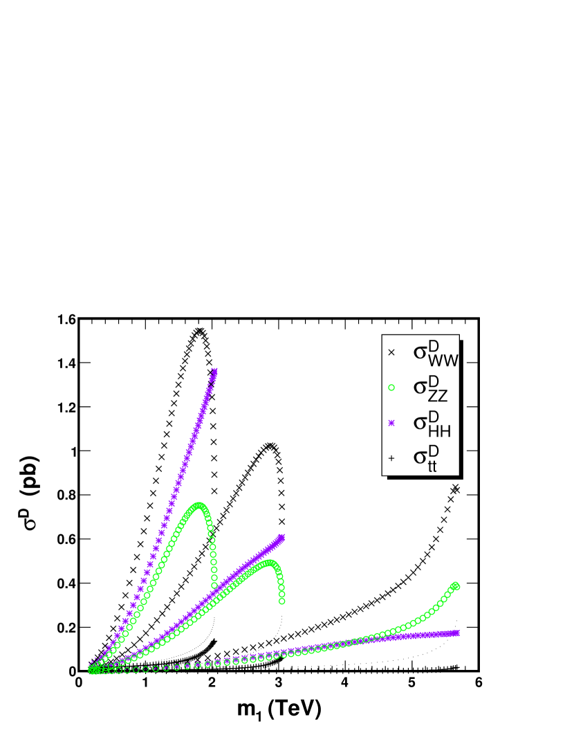
Figure 15: The cross-section contributions to the annihilation of the Dirac LOP for (from top to bottom) $\tilde{k}=1.5$, 2.2 and 3.8 TeV.

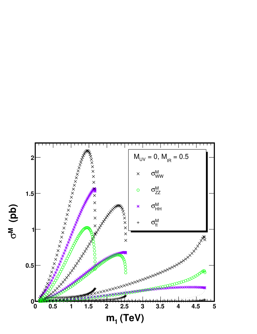
Figure 16: The cross-section contributions to the annihilation of the Majorana LOP with $M_{IR_{o}}=0.5$ and $M_{UV_{o}}=0$, for (from top to bottom) $\tilde{k}=1.5$, 2.2 and 3.8 TeV.

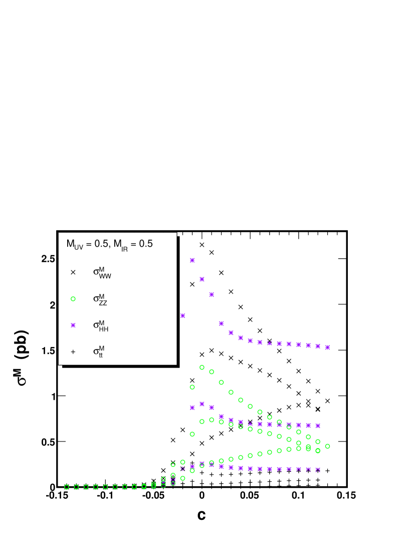
Figure 17: The cross-section contributions to the annihilation of the Majorana LOP with $M_{IR_{o}}=0.5$ and $M_{UV_{o}}=0.5$, for (from top to bottom) $\tilde{k}=1.5$, 2.2 and 3.8 TeV.

4.4 Dark Matter Density

We shall follow the standard formalism for the calculation of the thermal dark matter density [44], [45]. In calculating the annihilation cross-sections, we used the non-relativistic approximation for the initial particles. The cross-section used in calculating the dark matter density is the sum of all the different contributions in the previous sections and will be denoted by $<\sigma v>_{T}$, and $x_{F}=m/T_{F}$ as usual. The relative velocity is related to the freeze-out temperature:

$$<v^{2}>_{rel} = \frac{6}{x_{F}}\leavevmode\nobreak\ ,$$ (149)

$$x_{F} = \log\left(c\left(c+2\right)\sqrt{\frac{90\pi}{x_{F}g*}}\frac{g_{0}}{2\pi^{3}}m_{1}M_{Pl}<\sigma v>_{T}\right)\leavevmode\nobreak\ .$$ (150)

The non-relativistic expansion of the thermal annihilation cross section may be expressed as

$$<\sigma v>_{T}=\sigma_{0}+\sigma_{1}<v^{2}>\simeq\sigma_{0}+6\;\sigma_{1}/x_{F}.$$ (151)

The dark matter density is then given by

$$\Omega_{DM} = \frac{\gamma s_{0}x_{F}}{\rho_{c}M_{Pl}(\sigma_{0}+3\sigma_{1}/x_{F})}\sqrt{\frac{45}{\pi g*}},$$ (152)

where $c=1/2$, $M_{Pl}=1.2\times 10^{19}$ GeV, $g*=112$, $s_{0}=2889.2/\mbox{cm}^{3}$, $\rho_{c}=5.3\times 10^{-6}\mbox{GeV}/\mbox{cm}^{3}$, $g_{0}=2$ is the degrees of freedom of our dark matter candidate and $\gamma=2$ or $1$ to account for the antiparticles for the Dirac and Majorana case respectively. We take $g_{0}=2$ in the Dirac case since we compute the density of the particle and antiparticle separately. The factor $\gamma=2$ in the relic density then accounts for the duplication of the density from both the $N_{1}$ particle and the antiparticle in this case.

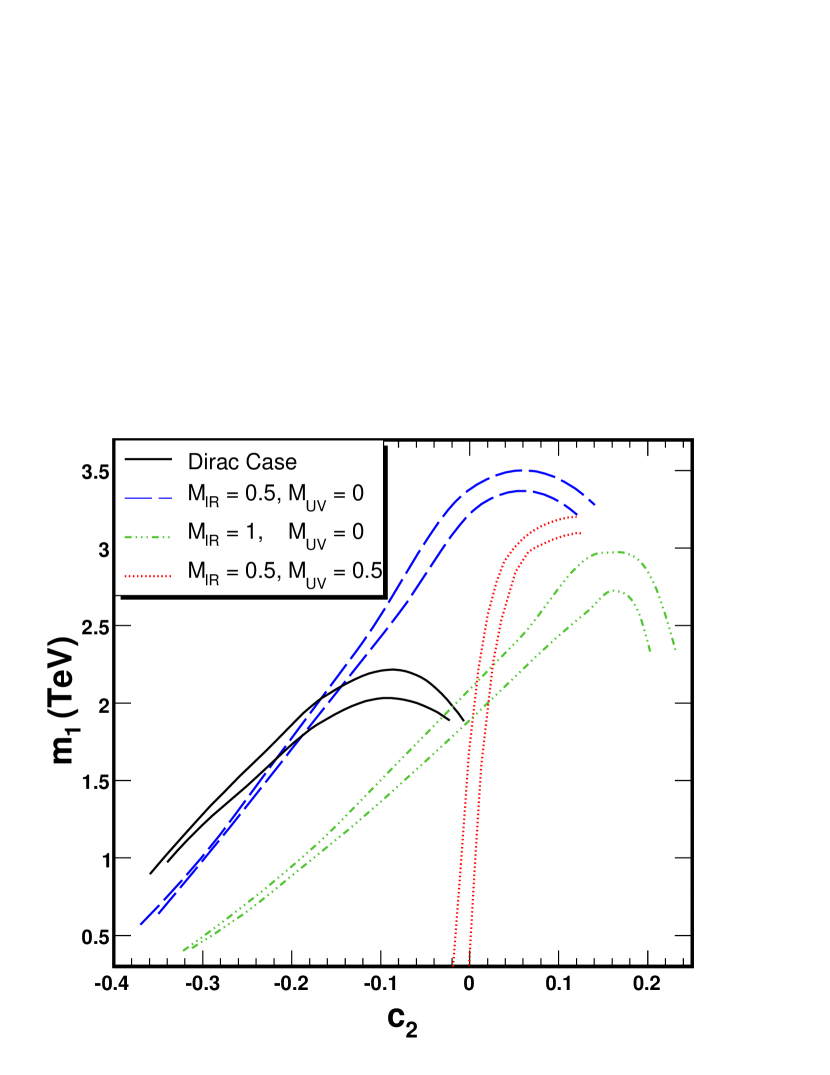
Figure 18: Parametric plot of $m_{1}$, the mass of the LOP, versus $c_{2}$, the localization parameter of the odd fermions, when $\Omega_{DM}\sim 0.23\pm 0.1$. The two lines for each value of the Majorana masses are associated with the upper and lower bound on $\Omega_{DM}$.

To check the veracity of our calculations, we extensively studied the limit of the Majorana case reducing to the Dirac case as $M_{IR_{o}}$ and $M_{UV_{o}}$ go to 0. As the Majorana masses go to 0, the two singlet masses start getting degenerate in mass, and the $N_{1}\leavevmode\nobreak\ N_{1}$ and the $N_{2}\leavevmode\nobreak\ N_{2}$ cross-sections become equal. To properly analyze this limit, then, we must take co-annihilation between the lightest Majorana sates into account [45]. One can check that the coupling of the Higgs to each of the degenerate LOP Majorana states, $HN_{i}N_{i}$, becomes equal to the one of the Higgs to the LOP in the Dirac case. Moreover, the cross coupling of the Higgs, $HN_{1}N_{2}$, vanishes identically in the limit of vanishing Majorana masses. Further simple relations exist between the Higgs couplings to fermions in the Majorana and Dirac cases. One can check that due to these relations the annihilation cross section into Higgs states in the Majorana case $N_{i}N_{i}\to H\leavevmode\nobreak\ H$ become the same as the $N_{1}\bar{N}_{1}\to H\leavevmode\nobreak\ H$ cross section in the Dirac case. The same happens in the case of annihilation into fermions.

In the case of gauge bosons the situation is more complicated. As noted in calculating the couplings, the gauge boson couplings in the Majorana case are reduced by a factor $1/\sqrt{2}$. This implies that for the $W^{\pm}$ and $Z\leavevmode\nobreak\ Z$, the interference between the t and s-channel diagrams is reduced by $1/2$ and the t-channel diagrams by $1/4$ compared to the Dirac cross-section case. These factors are exactly compensated for by the extra diagrams that contribute in the Majorana case (Fig. 14), and therefore one obtains that the equality of annihilation cross sections defined above for the Higgs final states extends to all final states. We also verified that the $N_{1}\leavevmode\nobreak\ N_{2}$ annihilation cross-section is exactly 0 in this limit. Including co-annihilation between the two Majorana states [45], the effective degrees of freedom are then 4, and the effective cross-section is $\frac{1}{2}\leavevmode\nobreak\ \sigma^{D}$, where $\sigma^{D}$ is the annihilation cross section between $N_{1}$ and its antiparticle in the Dirac case. Therefore, in this limit the dark matter density due to the Dirac and Majorana cases in the limit $M_{UV_{o},IR_{o}}\to 0$ is exactly the same, as expected.

We plotted the values of $c_{2}$ and $m_{1}$ leading to the correct dark matter density in both the Dirac and the Majorana cases in Fig. 18. We restricted the values of $\tilde{k}\stackrel{{\scriptstyle>}}{{{}_{\sim}}}1.2$ TeV, for which the SM Higgs couplings are close to their SM values. This provides a lower bound on the LOP mass and on the value of $c_{2}$. The bands in this figure represent the relic density uncertainty. We see that in the Dirac case, we can only obtain the correct dark matter density for values of $2$ TeV $\stackrel{{\scriptstyle>}}{{{}_{\sim}}}m_{1}\stackrel{{\scriptstyle>}}{{{}_{\sim}}}1$ TeV and $c_{2}\stackrel{{\scriptstyle>}}{{{}_{\sim}}}-0.4$, consistent with the exchange symmetry. The value of $\tilde{k}$ is correlated with the value of $m_{1}$, and is constrained to be in the range $2$ TeV $\stackrel{{\scriptstyle>}}{{{}_{\sim}}}\tilde{k}\stackrel{{\scriptstyle>}}{{{}_{\sim}}}1.2$ TeV for the above range of masses.

In the Majorana case, for $M_{UV_{o}}=0$, we are able to obtain the correct dark matter density for a larger range of $m_{1}$ values, which extend from about 3 TeV up to the lowest values of about $m_{1}\sim 500$ GeV, and for the range of negative values of $c_{2}\stackrel{{\scriptstyle>}}{{{}_{\sim}}}-0.4$. The values of $m_{1}$ are, again, correlated with the values of $\tilde{k}$, which is in the range $3$ TeV $\stackrel{{\scriptstyle>}}{{{}_{\sim}}}\tilde{k}\stackrel{{\scriptstyle>}}{{{}_{\sim}}}1.2$ TeV. For $M_{UV_{o}}\neq\leavevmode\nobreak\ 0$, instead, we see that we can only obtain the correct dark matter density for $c_{2}\stackrel{{\scriptstyle>}}{{{}_{\sim}}}0$. Due to the effect of the Majorana masses, the singlet LOP state mass is still significantly smaller than the doublet mass in this case and therefore co-annihilation effects may be ignored.

The values of $c_{2}$ obtained for the case of vanishing ultraviolet Majorana masses are fully compatible with the identification of the LOP with the odd partner of one of the right-handed neutrinos. Indeed, as can be seen from Fig. 2, for values of $c_{1}\simeq 0.5$–0.7, the proper neutrino masses are obtained for values of $-0.4\stackrel{{\scriptstyle<}}{{{}_{\sim}}}c_{2}\stackrel{{\scriptstyle<}}{{{}_{\sim}}}-0.1$, for which a proper dark matter candidate may be obtained, with a mass $0.5$ TeV $\stackrel{{\scriptstyle<}}{{{}_{\sim}}}m_{1}\stackrel{{\scriptstyle<}}{{{}_{\sim}}}2.5$ TeV.

The situation is different for non-vanishing values of the ultraviolet Majorana mass $M_{UV_{o}}$. In this case, a proper dark matter candidate may only be obtained for values of $c_{2}\stackrel{{\scriptstyle>}}{{{}_{\sim}}}0$. Such values of $c_{2}$ are incompatible with the exchange symmetry if the $c_{1}$’s of the three generations are approximately the same, as assumed in this article. Therefore, a proper dark matter candidate would demand that the Majorana mass at the UV brane is either zero or smaller than $\exp(2c_{2}k\;L)$, since in such a case, according to Eq. (121), masses of the order of the weak scale and couplings to the Higgs of order one would be obtained.

Observe that the difficulty in obtaining a proper dark matter candidate for $M_{UV_{o}}\neq 0$ stems from the fact that we have assumed equal bulk mass parameters for the fermions interchanged by the $Z_{2}$ exchanged symmetry introduced in Refs. [43]. Although this is an attractive possibility, since it allows a connection between the dark matter properties and the neutrino masses, this does not need to be the case. Values of $c_{2}\stackrel{{\scriptstyle>}}{{{}_{\sim}}}0$ would be allowed in the more general case, or for a more general discrete symmetry. Alternatively, if the value of $c_{1}$ of the left-handed leptons was allowed to be different for the three generations, values of $c_{2}\stackrel{{\scriptstyle>}}{{{}_{\sim}}}0$ would be consistent with values of $c_{1}$ compatible with the relatively small electron mass.

4.5 Direct Dark Matter Detection through Higgs Exchange

The annihilation cross section for the odd neutrinos becomes of the proper size for sizable values of the coupling of the odd neutrino to the Higgs boson, $\lambda_{11}\simeq 0.3$ – $0.7$, with larger couplings associated with larger LOP masses. Such large couplings induce a relatively large scattering cross section of the odd lepton with nuclei that may be probed at direct dark matter detection experiments. More quantitatively, the spin-independent elastic scattering cross-section for an odd lepton scattering off a heavy nucleus is:

$$\sigma_{SI}=\frac{4m_{r}^{2}}{\pi}\left(Zf_{p}+(A-Z)f_{n}\right)^{2}$$ (153)

where $m_{r}=\frac{m_{N}m_{N_{1}}}{m_{N}+m_{N_{1}}}$ and $m_{N}$ is the mass of the nucleus. The factors $f_{p,n}$ are given by

$$f_{p,n} = \left(\sum_{q=u,d,s}f_{T_{q}}^{(p,n)}\frac{a_{q}}{m_{q}}+\frac{2}{27}f_{TG}^{(p,n)}\sum_{q=c,b,t}\frac{a_{q}}{m_{q}}\right)m_{p,n}$$ (154)

$$a_{u,d} = -\frac{g_{2}m_{u,d}\lambda_{1,1}}{2m_{W}m_{H}^{2}},$$ (155)

where the quark form factors are $f_{T_{u}}^{p}=0.020\pm 0.004,f_{T_{d}}^{p}=0.026\pm 0.005,f_{T_{s}}^{p}=0.118\pm 0.062,f_{TG}^{p}\approx 0.84,f_{T_{u}}^{n}=0.014\pm 0.003,f_{T_{d}}^{n}=0.036\pm 0.008,f_{T_{s}}^{n}=0.118\pm 0.062$ and $f_{TG}^{n}\approx 0.83$ [46]. Hence, we find that the contribution is

$$f_{p,n} \approx -m_{p,n}\left(f_{T_{u}}^{p,n}+f_{T_{d}}^{p,n}+f_{T_{s}}^{p,n}+\frac{2}{27}f_{TG}^{p,n}\right)\frac{g_{2}\lambda_{11}}{2m_{W}m_{H}^{2}}$$ (156)

$$\approx -0.2m_{p}\frac{g_{2}\lambda_{11}}{2m_{W}m_{H}^{2}}$$ (157)

where we have neglected the differences between the proton and the neutron mass and have used the fact that the neutron and proton $f_{T}$ factors are relatively similar. Assuming that the mass of the odd neutrino is much larger than that of the nucleus we have $m_{r}\sim m_{N}\sim Am_{p}$ and

$$\sigma_{SI} \approx \frac{4A^{2}m_{p}^{2}}{\pi}A^{2}f_{p}^{2}$$ (158)

$$\Rightarrow\frac{\sigma_{SI}}{A^{4}} \approx \frac{0.04\;\lambda_{11}^{2}m_{p}^{4}g_{2}^{2}}{\pi m_{W}^{2}m_{H}^{4}},$$ (159)

where $\sigma_{SI}/A^{4}$ is the neutrino-nucleon spin-independent cross-section. From Eq. (159), the spin-independent cross-section scales as $\lambda_{11}^{2}/m_{H}^{4}$ and therefore direct dark matter detection experiments like CDMS can put strong constraints on regions of small $m_{H}$ and large $\lambda_{11}$.

As discussed above, in the Majorana case, an odd neutrino with a mass of about 700 GeV and a coupling to the Higgs of about 0.35 leads to an acceptable dark matter density. The spin independent cross section obtained in such a case for a Higgs mass, $m_{H}\simeq 130$ GeV, is about $1.4\times 10^{-43}$ cm². The current limit coming from CDMS, from a combination of the Ge data and under the standard assumptions of local dark matter density distribution, is about 2.5 $\times 10^{-43}$ cm² [47]. The XENON experiment puts a slightly weaker limit for this range of LOP masses [48]. Therefore, the predicted spin independent cross section is only a factor of a few lower than the current experimental limits. For larger masses, of about 1 TeV, the Higgs couplings grows to about 0.38 and the predicted cross section is therefore about $1.65\times 10^{-43}$ cm², while the CDMS bound is about two times larger. In the Dirac case, the couplings are about fifty percent larger than in the Majorana case and therefore the predicted cross section for a mass $m_{1}\simeq 1$ TeV is slightly above the CDMS reported bound. One would be able to conclude that the Dirac case for $m_{H}\stackrel{{\scriptstyle<}}{{{}_{\sim}}}130$ GeV is therefore disfavored. There are, however, uncertainties of order of a few associated with the local dark matter density distribution and the nuclear form factors which should be taken into account before ruling out a specific model. It is expected that both the XENON and CDMS experiments will further improve their sensitivity by about an order of magnitude by the end of 2009 [49], [50]. Therefore, even considering possible uncertainties associated with the local density and the nuclear form factors, the minimal model discussed in this article should be probed by these experiments in the near future.

Let us comment that the mass of the $N_{1}$ particle may be in the appropriate range to provide an explanation of the anomalous excess in electrons and positrons observed by the Pamela [51] and ATIC [52] experiments. However, since in these model these particles decay mostly into Higgs and gauge bosons, if these particles are distributed throughout the halo of the galaxy, an excess of positrons of the size observed by these experiments will need a large boost factor enhancement and would probably lead to an unobserved excess of antiprotons [53],[54].

5 Conclusions

In this article, we have considered the question of incorporating the charged and neutral leptons in a Gauge-Higgs Unification scenario based on the gauge group $SO(5)\times U(1)_{X}$ in warped extra dimensions. These models are attractive since the $SO(4)\equiv SU(2)_{L}\times SU(2)_{R}$ subgroup of $SO(5)$ incorporates in a natural way the weak gauge group as well as an appropriate custodial symmetry group in order to suppress large contributions to the precision electroweak observables. Moreover, the fifth dimensional components of $SO(5)/SO(4)$ gauge bosons have the right quantum numbers to play the role of the Higgs doublet responsible for the breakdown of the electroweak symmetry.

We have shown that, similar to the quark sector, the leptons can be incorporated by including the left-handed zero modes in a fundamental representation of $SO(5)$ and the right-handed charged leptons in a $\bf{10}$ of $SO(5)$. The model includes right-handed neutrinos which are singlets under the $SO(4)\times U(1)_{X}$ group and can therefore acquire localized Majorana masses on the IR and UV branes. The simple inclusion of the right-handed neutrinos in the same multiplet as the charged leptons, fails to produce the correct lepton masses. The correct charged lepton and neutrino masses may be obtained from a three multiplet structure similar to the quark case. The bulk mass parameters $c_{1}$, $c_{2}$ and $c_{3}$ of the left-handed leptons, right-handed neutrinos and right-handed charged leptons, respectively acquire values $c_{1}\simeq 0.5$ – 0.7, $-0.4\stackrel{{\scriptstyle<}}{{{}_{\sim}}}c_{2}\stackrel{{\scriptstyle<}}{{{}_{\sim}}}-0.1$ and $-0.9<c_{3}<-0.5$, where larger negative values of $c_{3}$ correspond to the first generation leptons.

We have further investigated the possibility of incorporating a dark-matter candidate by including an exchange symmetry, under which all SM leptons multiplets are even, and which ensures the stability of the lightest odd lepton partner. We therefore analyzed the possibility of associating the dark matter with the lightest neutral components of the odd leptons, transforming in the fundamental representation of $SO(5)$. We have shown that these neutral components have interesting properties. The neutral leptons that couple to the Higgs do not have self couplings to the $Z$-boson. However, these neutral states couple to the orthogonal combination of neutral states in the bidoublet and to the $Z$, as well as to the charged leptons and the $W$-gauge boson.

We computed the couplings of the neutral odd leptons to the gauge bosons and the Higgs in a functional way and computed the dominant contributions to the annihilation cross section into Higgs, neutral and charged gauge bosons and fermions (top-quark) final states. We considered the cases in which the Majorana masses for the neutral leptons vanish in both branes (Dirac case) as well as the case in which at least one of them is non-vanishing. By doing that, we have shown that in the Dirac case, a proper dark matter candidate may be obtained for masses of about 1 TeV to 2 TeV and localization parameter $-0.4\stackrel{{\scriptstyle<}}{{{}_{\sim}}}c_{2}\stackrel{{\scriptstyle<}}{{{}_{\sim}}}-0.1$ in agreement with the exchange symmetry. If only the Majorana mass in the infrared brane is non-vanishing, one obtains lower values of the required odd-lepton masses, which may be of about $500$ GeV to $2.5$ TeV, and a range for the localization parameter $-0.4\stackrel{{\scriptstyle<}}{{{}_{\sim}}}c_{2}\stackrel{{\scriptstyle<}}{{{}_{\sim}}}-0.1$. Finally, in the case that the Ultraviolet Majorana mass is different from zero, the self-couplings of the LOP with the Higgs is exponentially suppressed for $c_{2}<0$ and becomes non-vanishing only for $c_{2}\simeq 0$, for which a proper dark matter may be obtained with a mass similar to the one obtained when only $M_{IR}$ is different from zero. This last possibility is incompatible with the exchange symmetry and the proper neutrino masses if a common values of $c_{1}$ is assumed for the three families.

The collider signatures of these models have been previously discussed in the literature. The odd leptons introduced in this article will be hard to detect at collider experiments, since the masses of the charged and neutral non-LOP odd leptons are above a few TeV, and they have relatively weak interactions. In all cases, a proper dark matter candidate is obtained for values of the self-coupling of $N_{1}$ to the Higgs of about $0.3$ – $0.7$, with larger Higgs couplings corresponding to larger LOP masses, for which the cross section of the dark matter with nuclei becomes sizable. We have computed the dark matter cross section with nuclei and have shown that these models will be probed by the CDMS and XENON direct dark matter detection experiments in the near future.

Acknowledgments

We would like to thank Shri Gopalakrishna, Howard Haber, Eduardo Ponton, Jose Santiago and Tim Tait for useful discussions and comments. Work at ANL is supported in part by the US DOE, Div. of HEP, Contract DE-AC02-06CH11357. Fermilab is operated by Fermi Research Alliance, LLC under Contract No. DE-AC02-07CH11359 with the United States Department of Energy. We would like to thank the Aspen Center for Physics and the KITPC, China, where part of this work has been done.

APPENDIX

Appendix A Profile Functions at $h=0$.

In the $h=0$ gauge, we redefine $\hat{\psi}=a^{2}(x_{5})\psi$ and we write our vector-fermionic fields in terms of chiral fields. We can KK decompose the fermionic chiral components as,

$$\hat{\psi}_{L,R}=\sum_{n=0}^{\infty}\psi^{n}_{L,R}(x^{\mu})\hat{f}_{L,R,n}(x_{5})$$ (A.1)

where $\hat{f}$ is normalized by:

$$\int^{L}_{0}dx_{5}a^{-1}(x_{5})\hat{f}_{n}\hat{f}_{m}=\delta_{m,n}.$$ (A.2)

Therefore the profile function for the zero mode fermion corresponds to $a^{-1/2}(x_{5})\hat{f}_{0}$.

From the 5D action, concentrating on the free fermionic fields, we can derive the following first order coupled equations of motion for $\hat{f}_{L,R,n}$,

$$(\partial_{5}+M)\hat{f}_{R,n}=(z/a(x_{5}))\hat{f}_{L,n};\quad(\partial_{5}-M)\hat{f}_{L,n}=-(z/a(x_{5}))\hat{f}_{R,n}$$ (A.3)

We see from Eq. (A.3) that we can redefine $\tilde{f}_{R,L,n}=e^{-Mx_{5}}\hat{f}_{R,L,n}$ and relate the opposite chiral component of the same vector-like field by $\tilde{f}_{R,n}=(-a(x_{5})/z)\partial_{5}\tilde{f}_{L,n}$. For the left handed field having Dirichlet boundary conditions on the UV brane, we can derive a second order equation for the chiral component $\tilde{f}_{L,n}$:

$$\left[\partial_{5}^{2}+\left(\frac{a^{\prime}}{a}+2M\right)\partial_{5}+\frac{z^{2}}{a^{2}}\right]\tilde{f}_{L,n}=0$$ (A.4)

the solution of which we shall call $\tilde{S}_{M}(x_{5},z)$, with boundary conditions $\tilde{S}_{M}(0,z)=0$, $\tilde{S}_{M}^{\prime}(0,z)=z$.

Similarly, if the right-handed field fulfills Dirichlet boundary conditions on the UV-brane, we can redefine $\tilde{f}_{R,L,n}=e^{Mx_{5}}\hat{f}_{R,L,n}$ and then relate the opposite chirality via $\tilde{f}_{L,n}=(a(x_{5})/z)\partial_{5}\tilde{f}_{R,n}$. We can further write the equation of motion for $\tilde{f}_{R,n}$:

$$\left[\partial_{5}^{2}+\left(\frac{a^{\prime}}{a}-2M\right)\partial_{5}+\frac{z^{2}}{a^{2}}\right]\tilde{f}_{R,n}=0.$$ (A.5)

We shall correspondingly denote the solution to this equation with $\tilde{S}_{-M}(x_{5},z)$, fulfilling the boundary conditions $\tilde{S}_{-M}(0,z)=0$, $\tilde{S}_{-M}^{\prime}(0,z)=z$.

The solution to Eq. (A.4) is given by [3]:

$$\tilde{S}_{M}(x_{5},z)=\frac{\pi z}{2k}a^{-c-\frac{1}{2}}(x_{5})\left[J_{\frac{1}{2}+c}\left(\frac{z}{k}\right)Y_{\frac{1}{2}+c}\left(\frac{z}{ka(x_{5})}\right)-Y_{\frac{1}{2}+c}\left(\frac{z}{k}\right)J_{\frac{1}{2}+c}\left(\frac{z}{ka(x_{5})}\right)\right].$$ (A.6)

The solution for Eq. (A.5), $\tilde{S}_{-M}$, is given by Eq. (A.6) with the replacement $c\rightarrow-c$.

Appendix B Coupling of the charged gauge bosons

Following the notation of Ref. [26], the $W^{\pm}$ boson profile functions are given by:

$$f^{\hat{1}}_{G}(h) = S(x_{5})\left(\cos\left[\frac{\lambda h}{f_{h}}\right]C^{G}_{\hat{1}}+\frac{1}{\sqrt{2}}\sin\left[\frac{\lambda h}{f_{h}}\right]C^{G}_{1_{R}}\right)-\frac{1}{\sqrt{2}}C(x_{5})\sin\left[\frac{\lambda h}{f_{h}}\right]C^{G}_{1_{L}}$$ (B.1)

$$f^{1_{L}}_{G}(h) = \frac{1}{2}\left(S(x_{5})\left(\left(\cos\left[\frac{\lambda h}{f_{h}}\right]-1\right)C^{G}_{1_{R}}+\sqrt{2}\sin\left[\frac{\lambda h}{f_{h}}\right]C^{G}_{\hat{1}}\right)+C(x_{5})\left(1+\cos\left[\frac{\lambda h}{f_{h}}\right]\right)C^{G}_{1_{L}}\right)$$

$$f^{1_{R}}_{G}(h) = \frac{1}{2}\left(S(x_{5})\left(\left(\cos\left[\frac{\lambda h}{f_{h}}\right]+1\right)C^{G}_{1_{R}}-\sqrt{2}\sin\left[\frac{\lambda h}{f_{h}}\right]C^{G}_{\hat{1}}\right)+C(x_{5})\left(1-\cos\left[\frac{\lambda h}{f_{h}}\right]\right)C^{G}_{1_{L}}\right)$$

The normalization coefficients $C^{G}_{\hat{1},1_{R}}$, in terms of $C^{G}_{1_{L}}$ are given by:

$$C^{G}_{\hat{1}} = C^{G}_{1_{L}}\frac{-4\cos\left[\frac{\lambda h}{f_{h}}\right]_{L}C(L)^{\prime}S(L)^{\prime}+C_{h}he^{2kL}\sin\left[\frac{\lambda h}{f_{h}}\right]_{L}\left(C(L)^{\prime}S(L)+C(L)S(L)^{\prime}\right)}{\sqrt{2}S(L)^{\prime}\left(C_{h}he^{2kL}\cos\left[\frac{\lambda h}{f_{h}}\right]_{L}S(L)+2\sin\left[\frac{\lambda h}{f_{h}}\right]_{L}S(L)^{\prime}\right)}$$ (B.4)

$$C^{G}_{1_{R}} = -C^{G}_{1_{L}}\frac{C(L)^{\prime}}{S(L)^{\prime}}$$ (B.5)

The five dimensional weak coupling is defined as $g_{5w}=g_{w}\sqrt{L}$. In terms of these, the Dirac couplings for $W^{+}$ and $Z$, (denoted by $G$), are given by:

$$g^{D}_{G1_{L,R}2_{L,R}} = -g_{5w}\int^{L}_{0}\left(\vec{f}^{+,0^{\prime}}_{1_{L,R}}.\left(f^{\hat{1}}_{G}(h)T^{\hat{1}}+f^{1_{L}}_{G}(h)T^{1_{L}}+f^{1_{R}}_{G}(h)T^{1R}\right).\vec{f}^{\leavevmode\nobreak\ 0}_{2_{L,R}}\right)dx_{5}$$

$$= -g_{5w}\int^{L}_{0}\left(f^{1*}_{L,R}(h)\left(f^{5}_{L,R}(h)f^{\hat{1}}_{G}(h)+f^{2}_{L,R}(h)f^{1_{L}}_{G}(h)-f^{3}_{L,R}(h)f^{1_{R}}_{G}(h)\right)\right)dx_{5}$$

Again, due to our choice of normalization for the coefficient $C_{2}$, the factor $\sqrt{2}$, coming from the definition of the $W^{\pm}$ fields, is not present in this expression. The Majorana couplings are given in terms of the Dirac couplings,

$$g^{M}=\frac{1}{\sqrt{2}}g^{D},$$ (B.7)

with $g^{D}$ given in Eq. (LABEL:WLOP).

References

- [1] L. Randall and R. Sundrum, Phys. Rev. Lett. 83, 3370 (1999) [arXiv:hep-ph/9905221].
- [2] H. Davoudiasl, J. L. Hewett and T. G. Rizzo, Phys. Lett. B 473, 43 (2000) [arXiv:hep-ph/9911262].
- [3] A. Pomarol, Phys. Lett. B 486, 153 (2000) [arXiv:hep-ph/9911294].
- [4] S. Chang, J. Hisano, H. Nakano, N. Okada and M. Yamaguchi, Phys. Rev. D 62, 084025 (2000) [arXiv:hep-ph/9912498].
- [5] T. Gherghetta and A. Pomarol, Nucl. Phys. B 586, 141 (2000) [arXiv:hep-ph/0003129];
- [6] C. Csaki, J. Erlich and J. Terning, Phys. Rev. D 66, 064021 (2002) [arXiv:hep-ph/0203034].
- [7] J. L. Hewett, F. J. Petriello and T. G. Rizzo, JHEP 0209, 030 (2002) [arXiv:hep-ph/0203091].
- [8] H. Davoudiasl, J. L. Hewett and T. G. Rizzo, Phys. Rev. D 68, 045002 (2003) [arXiv:hep-ph/0212279].
- [9] M. S. Carena, E. Ponton, T. M. P. Tait and C. E. M. Wagner, Phys. Rev. D 67, 096006 (2003) [arXiv:hep-ph/0212307].
- [10] M. S. Carena, A. Delgado, E. Ponton, T. M. P. Tait and C. E. M. Wagner, Phys. Rev. D 68, 035010 (2003) [arXiv:hep-ph/0305188].
- [11] M. S. Carena, A. Delgado, E. Ponton, T. M. P. Tait and C. E. M. Wagner, Phys. Rev. D 71, 015010 (2005) [arXiv:hep-ph/0410344].
- [12] K. Agashe, A. Delgado, M. J. May and R. Sundrum, JHEP 0308, 050 (2003) [arXiv:hep-ph/0308036].
- [13] K. Agashe, R. Contino, L. Da Rold and A. Pomarol, Phys. Lett. B 641, 62 (2006) [arXiv:hep-ph/0605341].
- [14] M. Carena, E. Ponton, J. Santiago and C. E. M. Wagner, Nucl. Phys. B 759, 202 (2006) [arXiv:hep-ph/0607106].
- [15] M. S. Carena, E. Ponton, J. Santiago and C. E. M. Wagner, Phys. Rev. D 76, 035006 (2007) [arXiv:hep-ph/0701055].
- [16] N. Arkani-Hamed and M. Schmaltz, Phys. Rev. D 61, 033005 (2000) [arXiv:hep-ph/9903417].
- [17] Y. Grossman and M. Neubert, Phys. Lett. B 474, 361 (2000) [arXiv:hep-ph/9912408].
- [18] S. J. Huber and Q. Shafi, Phys. Lett. B 498, 256 (2001) [arXiv:hep-ph/0010195].
- [19] N. S. Manton, Nucl. Phys. B 158, 141 (1979); Y. Hosotani, Phys. Lett. B 126, 309 (1983); H. Hatanaka, T. Inami and C. S. Lim, Mod. Phys. Lett. A 13, 2601 (1998) [arXiv:hep-th/9805067]; I. Antoniadis, K. Benakli and M. Quiros, New J. Phys. 3, 20 (2001) [arXiv:hep-th/0108005]; M. Kubo, C. S. Lim and H. Yamashita, Mod. Phys. Lett. A 17, 2249 (2002) [arXiv:hep-ph/0111327]; C. Csaki, C. Grojean and H. Murayama, Phys. Rev. D 67, 085012 (2003) [arXiv:hep-ph/0210133]; N. Haba, M. Harada, Y. Hosotani and Y. Kawamura, Nucl. Phys. B 657, 169 (2003) [Erratum-ibid. B 669, 381 (2003)] [arXiv:hep-ph/0212035]; C. A. Scrucca, M. Serone and L. Silvestrini, Nucl. Phys. B 669, 128 (2003) [arXiv:hep-ph/0304220]; G. Burdman and Y. Nomura, Nucl. Phys. B 656, 3 (2003) [arXiv:hep-ph/0210257].
- [20] R. Contino, Y. Nomura and A. Pomarol, Nucl. Phys. B 671, 148 (2003) [arXiv:hep-ph/0306259].
- [21] K. Agashe and R. Contino, Nucl. Phys. B 742, 59 (2006) [arXiv:hep-ph/0510164].
- [22] R. Contino, L. Da Rold and A. Pomarol, Phys. Rev. D 75, 055014 (2007) [arXiv:hep-ph/0612048].
- [23] Y. Hosotani and M. Mabe, Phys. Lett. B 615, 257 (2005) [arXiv:hep-ph/0503020].
- [24] A. Falkowski, Phys. Rev. D 75, 025017 (2007) [arXiv:hep-ph/0610336].
- [25] A. D. Medina, N. R. Shah and C. E. M. Wagner, Phys. Rev. D 76, 095010 (2007) [arXiv:0706.1281 [hep-ph]].
- [26] M. Carena, A. D. Medina, B. Panes, N. R. Shah and C. E. M. Wagner, Phys. Rev. D 77, 076003 (2008) [arXiv:0712.0095 [hep-ph]].
- [27] K. Agashe, A. Belyaev, T. Krupovnickas, G. Perez and J. Virzi, arXiv:hep-ph/0612015.
- [28] B. Lillie, L. Randall and L. T. Wang, arXiv:hep-ph/0701166.
- [29] B. Lillie, J. Shu and T. M. P. Tait, arXiv:0706.3960 [hep-ph].
- [30] K. Agashe, G. Perez and A. Soni, Phys. Rev. D 75, 015002 (2007) [arXiv:hep-ph/0606293].
- [31] S. J. Huber and Q. Shafi, Phys. Lett. B 544, 295 (2002) [arXiv:hep-ph/0205327].
- [32] S. J. Huber and Q. Shafi, Phys. Lett. B 583, 293 (2004) [arXiv:hep-ph/0309252].
- [33] C. Csaki, A. Falkowski and A. Weiler, JHEP 0809, 008 (2008) [arXiv:0804.1954 [hep-ph]].
- [34] S. Casagrande, F. Goertz, U. Haisch, M. Neubert and T. Pfoh, JHEP 0810, 094 (2008) [arXiv:0807.4937 [hep-ph]].
- [35] A. L. Fitzpatrick, L. Randall and G. Perez, Phys. Rev. Lett. 100, 171604 (2008).
- [36] G. Perez and L. Randall, arXiv:0805.4652 [hep-ph].
- [37] M. C. Chen and H. B. Yu, arXiv:0804.2503 [hep-ph].
- [38] C. Csaki, C. Delaunay, C. Grojean and Y. Grossman, JHEP 0810, 055 (2008) [arXiv:0806.0356 [hep-ph]].
- [39] C. Csaki, A. Falkowski and A. Weiler, arXiv:0806.3757 [hep-ph].
- [40] J. Santiago, JHEP 0812, 046 (2008) [arXiv:0806.1230 [hep-ph]].
- [41] K. Agashe and G. Servant, Phys. Rev. Lett. 93, 231805 (2004) [arXiv:hep-ph/0403143].
- [42] K. Agashe, A. Falkowski, I. Low and G. Servant, JHEP 0804, 027 (2008) [arXiv:0712.2455 [hep-ph]].
- [43] G. Panico, E. Ponton, J. Santiago and M. Serone, Phys. Rev. D 77, 115012 (2008) [arXiv:0801.1645 [hep-ph]].
- [44] E. W. Kolb and M. S. Turner, Front. Phys. 69, 1 (1990).
- [45] K. Griest and D. Seckel, Phys. Rev. D 43, 3191 (1991).
- [46] G. B. Gelmini, P. Gondolo and E. Roulet, Nucl. Phys. B 351, 623 (1991). M. Srednicki and R. Watkins, Phys. Lett. B 225, 140 (1989). M. Drees and M. Nojiri, Phys. Rev. D 48, 3483 (1993) [arXiv:hep-ph/9307208]. J. R. Ellis, A. Ferstl and K. A. Olive, Phys. Lett. B 481, 304 (2000) [arXiv:hep-ph/0001005].
- [47] Z. Ahmed et al. [CDMS Collaboration], arXiv:0802.3530 [astro-ph].
- [48] J. Angle et al. [XENON Collaboration], Phys. Rev. Lett. 100, 021303 (2008) [arXiv:0706.0039 [astro-ph]].
- [49] http://xenon.astro.columbia.edu/presentations/Aprile_IDM08.pdf
- [50] T. Bruch [CDMS Collaboration], AIP Conf. Proc. 957, 193 (2007).
- [51] O. Adriani et al., arXiv:0810.4995 [astro-ph].
- [52] J. Chang et al., Nature 456, 362 (2008).
- [53] See, for example, M. Cirelli, M. Kadastik, M. Raidal and A. Strumia, arXiv:0809.2409 [hep-ph].
- [54] J. Hall and D. Hooper, arXiv:0811.3362 [astro-ph].