From Physics to Economics: An Econometric Example Using Maximum Relative Entropy

Abstract

Econophysics, is based on the premise that some ideas and methods from physics can be applied to economic situations. We intend to show in this paper how a physics concept such as entropy can be applied to an economic problem. In so doing, we demonstrate how information in the form of observable data and moment constraints are introduced into the method of Maximum relative Entropy (MrE). A general example of updating with data and moments is shown. Two specific econometric examples are solved in detail which can then be used as templates for real world problems. A numerical example is compared to a large deviation solution which illustrates some of the advantages of the MrE method.

1 Introduction

Methods of inference are not new to econometrics. In fact, one could say that the subject is founded on inference methods. Econophysics, on the other hand, is a much newer idea. It is based on the premise that some ideas and methods from physics can be applied to economic situations. In this paper we aim to show how a physics concept such as entropy can be applied to an economic problem.

In 1957, Jaynes [1] showed that maximizing statistical mechanic entropy for the purpose of revealing how gas molecules were distributed was simply the maximizing of Shannon’s information entropy [2] with statistical mechanical information. The method was true for assigning probabilities regardless of the information specifics. This idea lead to MaxEnt or his use of the Method of Maximum Entropy for assigning probabilities. This method has evolved to a more general method, the method of Maximum (relative) Entropy (MrE) [3, 4, 5] which has the advantage of not only assigning probabilities but updating them when new information is given in the form of constraints on the family of allowed posteriors. One of the draw backs of the MaxEnt method was the inability to include data. When data was present, one used Bayesian methods. The methods were combined in such a way that MaxEnt was used for assigning a prior for Bayesian methods, as Bayesian methods could not deal with information in the form of constraints, such as expected values. The main purpose of this paper is to show both general and specific examples of how the MrE method can be applied using data and moments.

The numerical example in this paper addresses a recent paper by Grendar and Judge (GJ) [6] where they consider the problem of criterion choice in the context of large deviations (LD). Specifically, they attempt to justify the method by Owen [7] in a LD context with a new method of their own. They support this idea by citing a paper in the econometric literature by Kitamura and Stutzer [8] who also use LD to justify a particular empirical estimator. We attempt to simplify their (GJ) initial problem by providing an example that is a bit more practical. However, our example has the same issue; what does one do when one has information in the form of an ”average” of a large data set and a small sample of that data set? We will show by example that the LD approach is a special case of our method, the method of Maximum (relative) Entropy

In section 2 we show a general example of updating simultaneously with two different forms of information: moments and data. The solution resembles Bayes’ Rule. In fact, if there are no moment constraints then the method produces Bayes rule exactly [9]. If there is no data, then the MaxEnt solution is produced. The realization that MrE includes not just MaxEnt but also Bayes’ rule as special cases is highly significant. It implies that MrE is capable of producing every aspect of orthodox Bayesian inference and proves the complete compatibility of Bayesian and entropy methods. Further, it opens the door to tackling problems that could not be addressed by either the MaxEnt or orthodox Bayesian methods individually; problems in which one has data and moment constraints.

In section 3 we comment on the problem of non-commuting constraints. We discuss the question of whether they should be processed simultaneously, or sequentially, and in what order. Our general conclusion is that these different alternatives correspond to different states of information and accordingly we expect that they will lead to different inferences.

In section 4, we provide two toy examples that illustrate potential economic problems similar to the ones discussed in GJ. The two examples (ill-behaved as mentioned in GJ) are solved in detail. The first example will demonstrate how data and moments can be processed sequentially. This example is typically how Bayesian statistics traditionally uses MaxEnt principles where MaxEnt is used to create a prior for the Bayesian formulation. The second example illustrates a problem that Bayes and MaxEnt alone cannot handle: simultaneous processing of data and moments. These two examples will seem trivially different but this is deceiving. They actually ask and answer two completely different questions. It is this ’triviality’ that is often a source of confusion in Bayesian literature and therefore we wish to expose it.

In section 6 we compare a numerical example that is solved by MrE and one that is solved by GJ’s method. Since GJ’s solution comes out of LD, they rely on asymptotic arguments; one assumes an infinite sample set which is not necessarily realistic. The MrE method does not need such assumptions to work and therefore can process finite amounts of data well. However, when MrE is taken to asymptotic limits one recovers the same solutions that the large deviation methods produce.

2 Simultaneous updating with moments and data

Our first concern when using the MrE method to update from a prior to a posterior distribution is to define the space in which the search for the posterior will be conducted. We wish to infer something about the values of one or several quantities, $\theta\in\Theta$, on the basis of three pieces of information: prior information about $\theta$ (the prior), the known relationship between $x$ and $\theta$ (the model), and the observed values of the data $x\in\mathcal{X}$. Since we are concerned with both $x$ and $\theta$, the relevant space is neither $\mathcal{X}$ nor $\Theta$ but the product $\mathcal{X}\times\Theta$ and our attention must be focused on the joint distribution $P\left(x,\theta\right)$. The selected joint posterior $P_{\text{new}}(x,\theta)$ is that which maximizes the entropy,

$$S[P,P_{\text{old}}]=-\int dxd\theta~{}P\left(x,\theta\right)\log\frac{P\left(x,\theta\right)}{P_{\text{old}}\left(x,\theta\right)}~{},$$ (1)

subject to the appropriate constraints. $P_{\text{old}}\left(x,\theta\right)$ contains our prior information which we call the joint prior. To be explicit,

$$P_{\text{old}}\left(x,\theta\right)=P_{\text{old}}\left(\theta\right)P_{\text{old}}\left(x|\theta\right)~{},$$ (2)

where $P_{\text{old}}\left(\theta\right)$ is the traditional Bayesian prior and $P_{\text{old}}\left(x|\theta\right)$ is the likelihood. It is important to note that they both contain prior information. The Bayesian prior is defined as containing prior information. However, the likelihood is not traditionally thought of in terms of prior information. Of course it is reasonable to see it as such because the likelihood represents the model (the relationship between $\theta$ and $x)$ that has already been established. Thus we consider both pieces, the Bayesian prior and the likelihood to be prior information.

The new information is the observed data, $x^{\prime}$, which in the MrE framework must be expressed in the form of a constraint on the allowed posteriors. The family of posteriors that reflects the fact that $x$ is now known to be $x^{\prime}$ is such that

$$P(x)=\int d\theta~{}P\left(x,\theta\right)=\delta\left(x-x^{\prime}\right)~{},$$ (3)

where $\delta\left(x-x^{\prime}\right)$ is the Dirac delta function. This amounts to an infinite number of constraints: there is one constraint on $P\left(x,\theta\right)$ for each value of the variable $x$ and each constraint will require its own Lagrange multiplier $\lambda(x)$. Furthermore, we impose the usual normalization constraint,

$$\int dxd\theta~{}P\left(x,\theta\right)=1~{},$$ (4)

and include additional information about $\theta$ in the form of a constraint on the expected value of some function $f\left(\theta\right)$,

$$\int dxd\theta\,P\left(x,\theta\right)f\left(\theta\right)=\left\langle f\left(\theta\right)\right\rangle=F~{}.$$ (5)

Note: an additional constraint in the form of $\int dxd\theta P(x,\theta)g(x)=\left\langle g\right\rangle=G$ could only be used when it does not contradict the data constraint (3). Therefore, it is redundant and the constraint would simply get absorbed when solving for $\lambda(x)$. We also emphasize that constraints imposed at the level of the prior need not be satisfied by the posterior. What we do here differs from the standard Bayesian practice in that we require the constraint to be satisfied by the posterior distribution.

We proceed by maximizing (1) subject to the above constraints. The purpose of maximizing the entropy is to determine the value for $P$ when $S=0.$ Meaning, we want the value of $P$ that is closest to $P_{\text{old}}$ given the constraints. The calculus of variations is used to do this by varying $P\rightarrow\delta P$, i.e. setting the derivative with respect to $P$ equal to zero. The Lagrange multipliers $\alpha,\beta$ and $\lambda(x)$ are used so that the $P$ that is chosen satisfies the constraint equations. The actual values are determined by the value of the constraints themselves. We now provide the detailed steps in this maximization process.

First we setup the variational form with the Lagrange multipiers,

$$\delta P\left(x,\theta\right)\left\{\begin{array}[]{c}S[P,P_{\text{old}}]+\alpha\left[\int dxd\theta P\left(x,\theta\right)-1\right]\\ +\beta\left[\int dxd\theta P\left(x,\theta\right)f\left(\theta\right)-F\right]\\ +\int dx\lambda(x)\left[\int d\theta P\left(x,\theta\right)-\delta\left(x-x{\acute{}}\right)\right]\end{array}\right\}=0~{}.$$ (6)

We expand the entropy function (1),

$$\delta P\left(x,\theta\right)\left\{\begin{array}[]{c}-\int dxd\theta~{}P\left(x,\theta\right)\log P\left(x,\theta\right)\\ +\int dxd\theta~{}P\left(x,\theta\right)\log P_{\text{old}}\left(x,\theta\right)\\ +\alpha\left[\int dxd\theta P\left(x,\theta\right)-1\right]\\ +\beta\left[\int dxd\theta P\left(x,\theta\right)f\left(\theta\right)-F\right]\\ +\int dx\lambda(x)\left[\int d\theta P\left(x,\theta\right)-\delta\left(x-x{\acute{}}\right)\right]\end{array}\right\}=0~{}.$$ (7)

Next, vary the functions with respect to $P\left(x,\theta\right),$

$$\left\{\begin{array}[]{c}-\int dxd\theta~{}\delta P\left(x,\theta\right)\log P\left(x,\theta\right)-\int dxd\theta~{}P\left(x,\theta\right)\frac{1}{P\left(x,\theta\right)}\delta P\left(x,\theta\right)\\ +\int dxd\theta~{}\delta P\left(x,\theta\right)\log P_{\text{old}}\left(x,\theta\right)+0\\ +\alpha\left[\int dxd\theta~{}\delta P\left(x,\theta\right)\right]\\ +\beta\left[\int dxd\theta~{}\delta P\left(x,\theta\right)f\left(\theta\right)\right]\\ +\int dx\lambda(x)\left[\int d\theta~{}\delta P\left(x,\theta\right)\right]\end{array}\right\}=0~{},$$ (8)

which can be rewritten as

$$\int dxd\theta\left\{-\log P\left(x,\theta\right)-1+\log P_{\text{old}}\left(x,\theta\right)+\alpha+\beta f\left(\theta\right)+\lambda(x)\right\}\delta P\left(x,\theta\right)=0~{}.$$

The terms inside the brackets must sum to zero, therefore we can write,

$$\log P\left(x,\theta\right)=\log P_{\text{old}}\left(x,\theta\right)-1+\alpha+\beta f\left(\theta\right)+\lambda(x)~{}$$ (9)

or

$$P_{\text{new}}\left(x,\theta\right)=P_{\text{old}}\left(x,\theta\right)e^{\left(-1+\alpha+\beta f\left(\theta\right)+\lambda(x)\right)}~{}$$ (10)

In order to determine the Lagrange multipliers, we substitute our solution (10) into the various constraint equations. The constant $\alpha$ is eleiminated by substituting (10) into (4),

$$\int dxd\theta~{}P_{\text{old}}\left(x,\theta\right)e^{\left(-1+\alpha+\beta f\left(\theta\right)+\lambda(x)\right)}=1~{}.$$ (11)

Dividing both sides by the constant $e^{\left(-1+\alpha\right)}$,

$$\int dxd\theta~{}P_{\text{old}}\left(x,\theta\right)e^{\beta f\left(\theta\right)+\lambda(x)}=e^{\left(1-\alpha\right)}~{}.$$ (12)

Then substituting back into (10) yields

$$P_{\text{new}}(x,\theta)=P_{\text{old}}\left(x,\theta\right)\frac{e^{\lambda(x)+\beta f\left(\theta\right)}}{Z}~{},$$ (13)

where

$$Z=e^{1-\alpha}=\int dxd\theta e^{\beta f\left(\theta\right)+\lambda(x)}P_{\text{old}}\left(x,\theta\right)~{}.$$ (14)

In the same fashion, the Lagrange multipliers $\lambda(x)$ are determined by substituting (13) into (3)

$$\int d\theta~{}P_{\text{old}}\left(x,\theta\right)\frac{e^{\lambda(x)+\beta f\left(\theta\right)}}{Z}=\delta\left(x-x^{\prime}\right)~{}$$ (15)

or

$$e^{\lambda(x)}=\frac{Z}{\int d\theta e^{\beta f\left(\theta\right)}P_{\text{old}}\left(x,\theta\right)}\delta(x-x{\acute{}})~{}.$$ (16)

The posterior now becomes

$$P_{\text{new}}(x,\theta)=P_{\text{old}}\left(x,\theta\right)\delta(x-x{\acute{}})\frac{e^{\beta f\left(\theta\right)}}{\zeta(x,\beta)}~{},$$ (17)

where $\zeta(x,\beta)=\int d\theta e^{\beta f\left(\theta\right)}P_{\text{old}}\left(x,\theta\right).$

The Lagrange multiplier $\beta$ is determined by first substituting (17) into (5),

$$\int dxd\theta\left[P_{\text{old}}\left(x,\theta\right)\delta(x-x{\acute{}})\frac{e^{\beta f\left(\theta\right)}}{\zeta(x,\beta)}\right]f\left(\theta\right)=F~{}.$$ (18)

Integrating over $x$ yields,

$$\frac{\int d\theta e^{\beta f\left(\theta\right)}P_{\text{old}}(x^{\prime},\theta)f\left(\theta\right)}{\zeta(x^{\prime},\beta)}=F~{},$$ (19)

where $\zeta(x,\beta)\rightarrow\zeta(x^{\prime},\beta)=\int d\theta e^{\beta f\left(\theta\right)}P_{\text{old}}(x^{\prime},\theta)$. Now $\beta$ can be determined rewriting (19) as

$$\frac{\partial\ln\zeta(x^{\prime},\beta)}{\partial\beta}=F~{}.$$ (20)

The final step is to marginalize the posterior, $P_{\text{new}}(x,\theta)$ over $x$ to get our updated probability,

$$P_{\text{new}}(\theta)=P_{\text{old}}(x^{\prime},\theta)\frac{e^{\beta f\left(\theta\right)}}{\zeta(x^{\prime},\beta)}$$ (21)

Additionally, this result can be rewritten using the product rule ($P\left(x,\theta\right)=P\left(x\right)P\left(\theta|x\right)$) as

$$P_{\text{new}}(\theta)=P_{\text{old}}\left(\theta\right)P_{\text{old}}(x^{\prime}|\theta)\frac{e^{\beta f\left(\theta\right)}}{\zeta^{\prime}\left(x^{\prime},\beta\right)}~{},$$ (22)

where $\zeta^{\prime}(x^{\prime},\beta)=\int d\theta e^{\beta f\left(\theta\right)}P_{\text{old}}\left(\theta\right)P_{\text{old}}(x^{\prime}|\theta).$ The right side resembles Bayes theorem, where the term $P_{\text{old}}(x^{\prime}|\theta)$ is the standard Bayesian likelihood and $P_{\text{old}}\left(\theta\right)$ is the prior. The exponential term is a modification to these two terms. In an effort to put some names to these pieces we will call the standard Bayesian likelihood the likelihood and the exponential part the likelihood modifier so that the product of the two gives the modified likelihood. The denominator is the normalization or marginal modified likelihood. Notice when $\beta=0$ (no moment constraint) we recover Bayes’ rule. For $\beta\neq 0$ Bayes’ rule is modified by a “canonical” exponential factor.

3 Commutivity of constraints

When we are confronted with several constraints, such as in the previous section, we must be particularly cautious. In what order should they be processed? Or should they be processed at the same time? The answer depends on the nature of the constraints and the question being asked [9].

We refer to constraints as commuting when it makes no difference whether they are processed simultaneously or sequentially. The most common example of commuting constraints is Bayesian updating on the basis of data collected in multiple experiments. For the purpose of inferring $\theta$ it is well known that the order in which the observed data $x^{\prime}=\{x_{1}^{\prime},x_{2}^{\prime},\ldots\}$ is processed does not matter. The proof that MrE is completely compatible with Bayes’ rule implies that data constraints implemented through $\delta$ functions, as in (3), commute just as they do in Bayes.

It is important to note that when an experiment is repeated it is common to refer to the value of $x$ in the first experiment and the value of $x$ in the second experiment. This is a dangerous practice because it obscures the fact that we are actually talking about two separate variables. We do not deal with a single $x$ but with a composite $x=(x_{1},x_{2})$ and the relevant space is $\mathcal{X}_{1}\times\mathcal{X}_{2}\times\Theta$. After the first experiment yields the value $x_{1}^{\prime}$, represented by the constraint $c_{1}:P(x_{1})=\delta\left(x_{1}-x_{1}^{\prime}\right)$, we can perform a second experiment that yields $x_{2}^{\prime}$ and is represented by a second constraint $c_{2}:P(x_{2})=\delta\left(x_{2}-x_{2}^{\prime}\right)$. These constraints $c_{1}$ and $c_{2}$ commute because they refer to different variables $x_{1}$ and $x_{2}$

As a side note, use of a $\delta$ function has been criticized in that by implementing it, the probability is completely constrained, thus it cannot be updated by future information. This is certainly true! An experiment, once performed and its outcome observed, cannot be un-performed and its result cannot be un-observed by subsequent experiments. Thus, imposing one constraint does not imply a revision of the other.

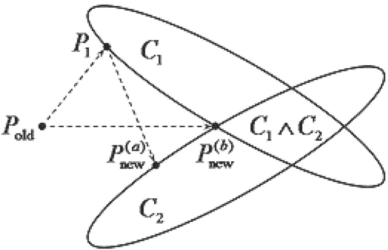
Figure 1: Illustrating the difference between processing two constraints $C_{1}$ and $C_{2}$ sequentially ($P_{\text{old}}\rightarrow P_{1}\rightarrow P_{\text{new}}^{(a)}$) and simultaneously ($P_{\text{old}}\rightarrow P_{\text{new}}^{(b)}$ or $P_{\text{old}}\rightarrow P_{1}\rightarrow P_{\text{new}}^{(b)}$).

In general constraints need not commute and when this is the case the order in which they are processed is critical. For example, suppose the prior is $P_{\text{old}}$ and we receive information in the form of a constraint, $C_{1}$. To update we maximize the entropy $S[P,P_{\text{old}}]$ subject to $C_{1}$ leading to the posterior $P_{1}$ as shown in Fig 1. Next we receive a second piece of information described by the constraint $C_{2}$. At this point we can proceed in essentially two different ways:

a) Sequential updating -

Having processed $C_{1}$, we use $P_{1}$ as the current prior and maximize $S[P,P_{1}]$ subject to the new constraint $C_{2}$. This leads us to the posterior $P_{\text{new}}^{(a)}$.

b) Simultaneous updating -

Use the original prior $P_{\text{old}}$ and maximize $S[P,P_{\text{old}}]$ subject to both constraints $C_{1}$ and $C_{2}$ simultaneously. This leads to the posterior $P_{\text{new}}^{(b)}$. At first sight it might appear that there exists a third possibility of simultaneous updating: (c) use $P_{1}$ as the current prior and maximize $S[P,P_{1}]$ subject to both constraints $C_{1}$ and $C_{2}$ simultaneously. Fortunately, and this is a valuable check for the consistency of the ME method, it is easy to show that case (c) is equivalent to case (b). Whether we update from $P_{\text{old}}$ or from $P_{1}$ the selected posterior is $P_{\text{new}}^{(b)}$.

To decide which path (a) or (b) is appropriate, we must be clear about how the MrE method treats constraints. The MrE machinery interprets a constraint such as $C_{1}$ in a very mechanical way: all distributions satisfying $C_{1}$ are in principle allowed and all distributions violating $C_{1}$ are ruled out.

Updating to a posterior $P_{1}$ consists precisely in revising those aspects of the prior $P_{\text{old}}$ that disagree with the new constraint $C_{1}$. However, there is nothing final about the distribution $P_{1}$. It is just the best we can do in our current state of knowledge and we fully expect that future information may require us to revise it further. Indeed, when new information $C_{2}$ is received we must reconsider whether the original $C_{1}$ remains valid or not. Are all distributions satisfying the new $C_{2}$ really allowed, even those that violate $C_{1}$? If this is the case then the new $C_{2}$ takes over and we update from $P_{1}$ to $P_{\text{new}}^{(a)}$. The constraint $C_{1}$ may still retain some lingering effect on the posterior $P_{\text{new}}^{(a)}$ through $P_{1},$ but in general $C_{1}$ has now become obsolete.

Alternatively, we may decide that the old constraint $C_{1}$ retains its validity. The new $C_{2}$ is not meant to revise $C_{1}$ but to provide an additional refinement of the family of allowed posteriors. In this case the constraint that correctly reflects the new information is not $C_{2}$ but the more restrictive space where $C_{1}$ and $C_{2}$ overlap. The two constraints should be processed simultaneously to arrive at the correct posterior $P_{\text{new}}^{(b)}$.

To summarize: sequential updating is appropriate when old constraints become obsolete and are superseded by new information; simultaneous updating is appropriate when old constraints remain valid. The two cases refer to different states of information and therefore we expect that they will result in different inferences. These comments are meant to underscore the importance of understanding what information is being processed; failure to do so will lead to errors that do not reflect a shortcoming of the MrE method but rather a misapplication of it.

4 An econometric problem: sequential updating

This is an example of a problem using the MrE method:. The general background information is that a factory makes $k$ different kinds of bouncy balls. For reference, they assign each different kind with a number, $f_{1},f_{2},...f_{k}$. They ship large boxes of them out to stores. Unfortunately, there is no mechanism that regulates how many of each ball goes into the boxes, therefore we do not know the amount of each kind of ball in any of the boxes.

For this problem we are informed that the company does know the average of all the kinds of balls, $F$ that is produced by the factory over the time that they have been in existence. This is information about the factory. By using this information with MrE we get what one would get with the old MaxEnt method, a distribution of balls for the whole factory.

However, we would like to know the probability of getting a certain kind of ball in a particular box. Therefore, we are allowed to randomly select a few balls, $n$ from the particular box in question and count how many of each kind we get, $m_{1},m_{2}...m_{k}$ (or perhaps we simply open the box and look at the balls on the surface). This is information about the particular box. Now let us put the above example in a more mathematical format.

Let the set of possible outcomes be represented by, $\Omega=\{f_{1},f_{2},...f_{k}\}$ from a sample where the total number of balls, $N\rightarrow\infty$ and whose sample average is $F.$ Further, let us draw a data sample of size $n,$ from a particular subset of the original sample, $\omega$ where $\omega\in\Omega$ and whose outcomes are counted and represented as $m=(m_{1},m_{2}...m_{k})$ where $n=\sum\nolimits_{i}^{k}m_{i}$. We would like to determine the probability of getting any particular type in one draw ($\theta=\{\theta_{1},\theta_{2}...\theta_{k}\}$) out of the subset given the information. To do this we start with the appropriate joint entropy,

$$S[P,P_{\text{old}}]~{}\text{=}-\sum\limits_{m}\int d\theta P(m,\theta|n)\log\frac{P\left(m,\theta|n\right)}{P_{\text{old}}(m,\theta|n)}.$$ (23)

We then maximize this entropy with respect to $P(m,\theta|n)$ to process the first piece of information that we have which is the moment constraint, $C_{1}$ that is related to the factory,

$$C_{1}:\left\langle f\left(\theta\right)\right\rangle=F\quad\text{where}\quad f\left(\theta\right)=\sum\nolimits_{i}^{k}f_{i}\theta_{i}~{},$$ (24)

subject to normalization, where $\theta=\{\theta_{1},\theta_{2}...\theta_{k}\},$ $m=\left(m_{1}...m_{k}\right)$ and where

$$\sum\limits_{m}=\sum\limits_{m_{1}\ldots m_{k}=0}^{n}\delta\left(\sum\nolimits_{i=1}^{k}m_{i}-n\right)~{},$$ (25)

and

$$\int d\theta=\int d\theta_{1}\ldots d\theta_{k}\,\delta\left(\sum\nolimits_{i=1}^{k}\theta_{i}-1\right)~{}.$$ (26)

This yields,

$$P_{\text{1}}(m,\theta|n)=P_{\text{old}}(m,\theta|n)\frac{e^{\lambda f\left(\theta\right)}}{Z_{1}}~{},$$ (27)

where the normalization constant $Z_{1}$ and the Lagrange multiplier $\lambda$ are determined from

$$Z_{1}=\int d\theta\,e^{\lambda f\left(\theta\right)}P_{\text{old}}(\theta|n)\quad\text{and}\quad\frac{\partial\log Z_{1}}{\partial\lambda}=F~{}.$$ (28)

We need to determine what to use for our joint prior,

$$P_{\text{old}}(m,\theta|n)=P_{\text{old}}(m^{\prime}|\theta,n)P_{\text{old}}(\theta|n)$$ (29)

in our problem. The mathematical representation of the situation where we wish to know the probability of selecting $m_{i}$ balls of the $i^{th}$ type from a sample of $n$ balls of $k$-types is simply the multinomial distribution. Therefore, the equation that we will use for our model, the likelihood, $P_{\text{old}}(m^{\prime}|\theta,n)$ is,

$$P_{\text{old}}(m_{1}...m_{k}|\theta_{1}...\theta_{k},n)=\frac{n!}{m_{1}!...m_{k}!}\theta_{1}^{m_{1}}..\theta_{k}^{m_{k}}~{}.$$ (30)

Since at this point we are completely ignorant of $\theta,$ we use a prior that is flat, thus $P_{\text{old}}(\theta|n)=$ constant. Being a constant, the prior can come out of the integral and cancels with the same constant in the numerator. (Also, the particular form of $P_{\text{old}}(\theta|n)$ is not important for our current purpose so for the sake of definiteness we can choose it flat for our example. There are most likely better choices for priors, such as a Jeffrey’s prior.) Thus, after marginalizing over $m,$ the joint distribution (27) can be rewritten as

$$P_{1}(\theta)=\frac{e^{\lambda f\left(\theta\right)}}{Z_{1}}~{}.$$ (31)

Now we wish to process the next piece of information which is the data constraint,

$$C_{2}:P(m)=\delta_{mm^{\prime}}~{}.$$ (32)

Here we use a Kronecker delta function since $m$ is discrete in this example. Our goal is to infer the $\theta$ that apply to our particular box. The original constraint $C_{1}$ applies to the whole factory while the new constraint $C_{2}$ refers to the actual box of interest and thus takes precedence over $C_{1}.$ As $n\rightarrow\infty$ we expect $C_{1}$ to become less and less relevant. Therefore the two constraints should be processed sequentially.

We maximize again with our new information which yields,

$$P_{\text{new}}^{(a)}(m,\theta)=\delta_{mm^{\prime}}P_{1}(\theta|m)~{}.$$ (33)

Marginalizing over $m$ and using (31) the final posterior for $\theta$ is

$$P_{\text{new}}^{(a)}(\theta)=P_{1}(\theta|m^{\prime})=P_{\text{old}}(m^{\prime}|\theta)\frac{e^{\lambda f\left(\theta\right)}}{Z_{2}}~{}.$$ (34)

where

$$Z_{2}=\int d\theta\,e^{\lambda f\left(\theta\right)}P_{\text{old}}(m^{\prime}|\theta)~{}.$$ (35)

Those familiar with using MaxEnt and Bayes will undoubtedly recognize that (34) is precisely the result obtained by using MaxEnt to obtain a prior, in this case $P_{1}(\theta)$ given in (31), and then using Bayes’ rule to take the data into account. This familiar result has been derived in detail for two reasons: first, to reassure the readers that MrE does reproduce the standard solutions to standard problems and second, to establish a contrast with the example discussed next. NOTE: Since the constraints $C_{1}$ and $C_{2}$ do not commute one will get a different result if they are processed in a different order.

5 An econometric problem: simultaneous updating

This is another example of a problem using the MrE method:. The general background information is the same as the previous example. For this problem we are informed that the company knows the average of all the kinds of balls, $F$ in each box. By using this information with MrE we get what one would get with the old MaxEnt method, a distribution of balls for each box.

However, we still would like to know the probability of getting a certain kind of ball in a particular box and we are allowed to randomly select a few balls, $n$ from the particular box in question once again. Since both of these pieces of information apply to the same box, they must be processed simultaneously. In other words, both constraints must hold, always. We proceed as in the first example by maximizing (23) subject to normalization and the following constraints simultaneously,

$$C_{3}:\left\langle f\left(\theta\right)\right\rangle=F\quad\text{where}\quad f\left(\theta\right)=\sum\nolimits_{i}^{k}f_{i}\theta_{i}~{},$$ (36)

(notice $C_{3}\neq C_{1}$ because they are two difference pieces of information) and

$$C_{2}:P(m)=\delta_{mm^{\prime}}~{}.$$ (37)

This yields,

$$P_{\text{new}}^{(b)}(\theta)=P_{1}(\theta|m^{\prime})=P_{\text{old}}(m^{\prime}|\theta)\frac{e^{\beta f\left(\theta\right)}}{\zeta}~{},$$ (38)

where

$$\zeta=\int d\theta\,e^{\beta f\left(\theta\right)}P_{\text{old}}(m^{\prime}|\theta)~{},$$ (39)

and

$$F=\frac{\partial\log\zeta}{\partial\beta}~{}.$$ (40)

This looks like the sequential case (34), but there is a crucial difference: $\beta\neq\lambda$ and $\zeta\neq Z_{2}$. In the sequential updating case, the multiplier $\lambda$ is chosen so that the intermediate $P_{1}$ satisfies $C_{1}$ while the posterior $P_{\text{new}}^{(a)}$ only satisfies $C_{2}$. In the simultaneous updating case the multiplier $\beta$ is chosen so that the posterior $P_{\text{new}}^{(b)}$ satisfies both $C_{1}$ and $C_{2}$ or $C_{1}\wedge C_{2}$. Ultimately, the two distributions $P_{\text{new}}(\theta)$ are different because they refer to different problems. For more examples using this method see [9].

6 Numerical examples

The purpose of this section is two fold: First, we would like to provide a numerical example of a MrE solution. Second, we wish to examine a current, relevant econometric solution proposed by GJ in [6] using the method of types, specifically large deviation theory, for an ”ill-posed” problem that is similar to the one discussed in section 5. This solution will be compared with a solution using MrE.

To summarize the problem once again: The factory makes $k$ different kinds of bouncy balls and for reference, they assign each different type with a number, $f_{1},f_{2},...f_{k}$. We are informed that the company knows the expected type of ball, $F$ in each box over the time that they have been in existence. We would like a better idea of how many balls are in each box so we randomly select a few balls, $n$ from a particular box and count how many of each type we get, $m_{1},m_{2}...m_{k}$.

Or stated in a more mathematical format: Let the set of possible outcomes of a be represented by, $\Omega=\{f_{1},f_{2},...f_{k}\}$ from a sample where the total number of balls, $N\rightarrow\infty$. and where the average of the types of balls is $F.$ Further, let us draw a data sample of size $n,$ from the original sample, whose outcomes are counted and represented as $m=(m_{1},m_{2}...m_{k})$ where $n=\sum\nolimits_{i}^{k}m_{i}$. The problem becomes ill-posed when the sample average of the counts

$$S_{Avg}=\frac{1}{n}\sum_{i}f_{i}m_{i}$$ (41)

significantly deviates from the expected average of the types, $F.$

We would like to determine the probability of getting any particular outcome in one draw ($\theta=\{\theta_{1},\theta_{2}...\theta_{k}\}$) given the information.

6.1 Sanov’s theorem solution

In [6] a form of Sanov’s theorem is used. Here we give a brief description of Sanov’s theorem. It is not intended to be a proof or exhaustive. It is simply shown to give a general indication of the basis for the solution in [6]. The key equation is (46). For a more detailed proof and explanation see [10].

Sanov’s theorem -

Let $X_{1}\ldots X_{n}$ be independent and identically distributed (i.i.d.) with values in an arbitrary set $\chi$ with common distribution $Q(x)$. Let $E\subseteq\mathcal{P}$ be a set of probability distributions. Then,

$$Q^{n}(E)=Q^{n}(E\cap\mathcal{P}_{n})\leq(n+1)^{\left|\mathcal{X}\right|}2^{-nD(P^{\ast}||Q)}~{},$$ (42)

where

$$P^{\ast}=\arg\min_{P\in E}D(P||Q)$$ (43)

is the distribution in $E$ that is closest to $Q$ in the relative entropy or information divergence,

$$D(P||Q)=\sum\limits_{x\in\chi}dxP(x)\log\frac{P\left(x\right)}{Q(x)}$$ (44)

and $n$ is the number of types. If in addition, the set $E$ is the closure of its interior,

$$\frac{1}{n}\log Q^{n}(E)\rightarrow-D(P^{\ast}||Q)~{}.$$ (45)

The two equations become equal in the asymptotic limit. Essentially what this theorem says is that in the asymptotic limit, the frequency of the sample $Q$, can be used to produce an estimate, $P^{\ast}$ of the ”true” probability, $\mathcal{P}$ by way of minimizing the relative entropy (44).

For our problem, the solution for the probability using Sanov is of the form,

$$P^{\ast}=\frac{Qe^{\eta_{i}f_{i}}}{\sum_{i}Qe^{\eta_{i}f_{i}}}~{},$$ (46)

where $Q$ for our problem is the frequency of the counts, $m/n$ and $\eta$ is a Lagrange multiplier that is determined by the sample average (41), not an expected value as in our method. This solution seems very similar to our general solution using the MrE method (38) in which we also minimize an entropy (maximize our negative relative entropy). We could even think of $Q$ as a kind of joint prior and likelihood. However, there are many differences in the two methods, but the most glaring is that the GJ solution is only valid in the asymptotic case. We are not handicapped by this when MrE is used.

6.2 Comparing the methods

We illustrate the differences between the methods be examining a specific version of the above problem: Let the there be three kinds of balls labeled 1, 2 and 3. So for this problem we have $f_{1}=1,$ $f_{2}=2$ and $f_{3}=3.$ Further, we are given information regarding the expected value of each box, $F.$ For our example this value will be, $F=2.3.$ Notice that this implies that on the average there are more $3$’s in each box. Next we take a sample of one of the boxes where $m_{1}^{\prime}=11,$ $m_{2}^{\prime}=2$ and $m_{3}^{\prime}=7.$

Using the MrE method in the same way that we have in each of the previous sections, we arrive at a posterior solution after maximizing the proper entropy subject to the constraints,

$$P_{\text{MrE}}(\theta_{1},\theta_{2})=\frac{1}{\zeta_{\text{MrE}}}e^{\beta(-2\theta_{1}-\theta_{2}+3)}\theta_{1}^{11}\theta_{2}^{2}(1-\theta_{1}-\theta_{2})^{7}~{}.$$ (47)

where the Lagrange multiplier $\beta$ was determined using Newton’s method on the equation (40) and found to be $\beta=14.1166.$ We show the relationship between $\beta$ and $F$ in Fig 2.

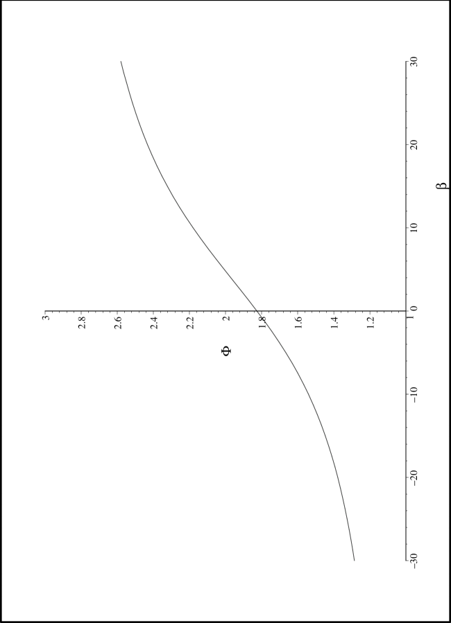
Figure 2: This figure shows the relationship between $\beta$ and $\Phi(\Phi=F(\beta)).$ Notice that as the value for $\Phi$ approaches the extremities of the outcomes, $\beta$ approaches infinity.

This result is then put into our calculation of $\zeta_{\text{MrE}}$ so that $\zeta_{\text{MrE}}=1874.1247.$ Two plots are provided that show the marginal distributions of $\theta_{1}$ and $\theta_{2}$ (see Fig 3). One may choose to have a single number represent $\theta_{1},\theta_{2}$ and $\theta_{3}.$ A popular choice is the mean, which is calculated for each marginal (see appendix for details),

$$\left\langle\theta_{1}\right\rangle=0.2942,~{}\left\langle\theta_{2}\right\rangle=0.1115,~{}\left\langle\theta_{3}\right\rangle=0.5942$$ (48)

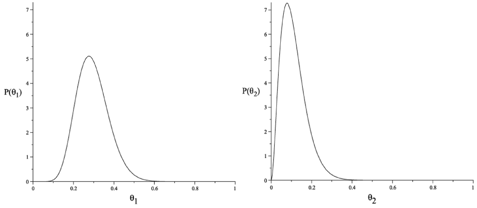
Figure 3: These figures show the distributions of $\theta_{1}$ and $\theta_{2}$ respectively.

We now use the GJ solution (46) to compute the ”probabilities”. We use the frequencies, $m/n$ for $Q$ or $Q_{1}=11/20,$ $Q_{2}=2/20$ and $Q_{3}=7/20$ and assume that $F$ represents the sample average for the entire population of balls. This produces the following results:

$$P_{1}^{\ast}=0.3015,~{}P_{2}^{\ast}=0.0971,~{}P_{3}^{\ast}=0.6015_{.}$$ (49)

Clearly the results are very close, however, there are several drawbacks to using the Sanov approach. The first is that $P^{\ast}$ is estimated on the basis of a frequency, $Q$ that is being used to represent an estimate of the entire population. As is well known this can only be the case when $n\rightarrow\infty.$ MrE needs not make such assumptions. Similarly MrE can incorporate actual expectation values, not sample averages disguised as them. Second, the correct distribution to be used is the multinomial when one is counting, not the frequencies of the observables. Third, and practically most important, because the MrE solution produces a probability distribution, one can take into account fluctuations. A single number would not give any indication as to the uncertainty of the estimate. With our method, one has the choice of which estimator one would like to use. Perhaps the distribution is almost flat. Then our method would indicate that almost any choice is equally likely. There is an underlying theme here: probabilities are not equivalent to frequencies except in the asymptotic case. Therefore, if one wishes to know the probable outcome of a problem in all cases, use MrE.

7 Conclusions

The realization that the MrE method incorporates MaxEnt and Bayes’ rule as special cases has allowed us to go beyond Bayes’ rule and MaxEnt methods to process both data and expected value constraints simultaneously. Therefore, we would like to emphasize that anything one can do with Bayesian or MaxEnt methods, one can now do with MrE. Additionally, in MrE one now has the ability to apply additional information that Bayesian or MaxEnt methods could not. Further, any work done with Bayesian techniques can be implemented into the MrE method directly through the joint prior.

It is not uncommon to claim that the non-commutability of constraints represents a problem for the MrE method. Processing constraints in different orders might lead to different inferences. We have argued that on the contrary, the information conveyed by a particular sequence of constraints is not the same information conveyed by the same constraints in different order. Since different informational states should in general lead to different inferences, the way MrE processes non-commuting constraints should not be regarded as a shortcoming but rather as a feature of the method.

Two specific econometric examples were solved in detail to illustrate the application of the method. These cases can be used as templates for real world problems. Numerical results were obtained to illustrate explicitly how the method compares to other methods that are currently employed. The MrE method was shown to be superior in that it did not need to make asymptotic assumptions to function and allows for fluctuations.

It must be emphasized that in the asymptotic limit, the MrE form is analogous to Sanov’s theorem. However, this is only one special case. The MrE method is more robust in that it can also be used to solve traditional Bayesian problems. In fact it was shown that if there is no moment constraint one recovers Bayes rule.

Acknowledgements: I would like to acknowledge valuable discussions with A. Caticha, M. Grendar, C. Rodríguez and E. Scalas.

Appendix A Solving the normalization factor

Here we show how the means $\left\langle\theta_{1}\right\rangle,\left\langle\theta_{2}\right\rangle$ and $\left\langle\theta_{3}\right\rangle$ were calculated explicitly in the numerical solutions section. The program Maple was used to calculate all results after the integral from was created.

In general, we rewrite the posterior (38) in more detail, dropping the superscripts,

$$P_{\text{new}}(\theta)=\frac{1}{\zeta^{\prime}}\delta(\sum\limits_{i}^{k}\theta_{i}-1)\prod\limits_{i=1}^{k}e^{\beta f_{i}\theta_{i}}\theta_{i}^{m_{i}^{\prime}}.$$ (50)

where $\zeta^{\prime}$ differs from $\zeta$ in (39) only by a combinatorial coefficient,

$$\zeta^{\prime}=\int\delta(\sum\limits_{i}^{k}\theta_{i}-1)\prod\limits_{i=1}^{k}d\theta_{i}e^{\beta f_{i}\theta_{i}}\theta_{i}^{m_{i}^{\prime}}~{}.$$ (51)

A brute force calculation gives $\zeta^{\prime}$ as a nested hypergeometric series,

$$\zeta^{\prime}=e^{\beta f_{k}}I_{1}(I_{2}(\ldots(I_{k-1})))\,,$$ (52)

where each $I$ is written as a sum of $\Gamma$ functions,

$$I_{j}=\Gamma(b_{j}-a_{j})\sum\limits_{q_{j}=0}^{\infty}\frac{\Gamma(a_{j}+q_{j})}{\Gamma(b_{j}+q_{j})~{}q_{j}!}t_{j}^{q_{j}}I_{j+1}~{},$$ (53)

where $I_{k}=1.$ The index $j$ takes all values from $1$ to $k-1$ and the other symbols are defined as follows: $t_{j}=\beta\left(f_{k-j}-f_{k}\right)$, $a_{j}=m_{k-j}^{\prime}+1$ and

$$b_{j}=n+j+1+\sum\limits_{i=0}^{j-1}q_{i}-\sum\limits_{i=0}^{k-j-1}m_{i}^{\prime}~{}\,,$$ (54)

with $q_{0}=m_{0}^{\prime}=0$. The terms that have indices $=0$ are equal to zero (i.e. $b_{0}=q_{0}=0,$ etc.). A few technical details are worth mentioning: First, one can have singular points when $t_{j}=0$. In these cases the sum must be evaluated in the limit as $t_{j}\rightarrow 0.$ Second, since $a_{j}$ and $b_{j}$ are positive integers the gamma functions involve no singularities. Lastly, the sums converge because $a_{j}>b_{j}$. The normalization for the first example (35) can be calculated in a similar way.

Specifically for (47), the Lagrange multiplier $\beta$ was determined using Newton’s method on the equation (40) and found to be $\beta=14.1166.$ This result is then put into (52) in order to attain $\zeta^{\prime}=1874.1247.$ Next, the means were calculated by increasing $m_{i}+1$ and $n+1,$ then recalculating so that

$$\begin{array}[]{l}\left\langle\theta_{1}\right\rangle=\frac{\zeta_{m_{1}+1,n+1}^{\prime}}{\zeta^{\prime}}~{},\\ \left\langle\theta_{2}\right\rangle=\frac{\zeta_{m_{2}+1,n+1}^{\prime}}{\zeta^{\prime}}~{},\\ \left\langle\theta_{3}\right\rangle=1-\left\langle\theta_{1}\right\rangle-\left\langle\theta_{2}\right\rangle~{}.\end{array}$$ (55)

Currently, for small values of $k$ (less than 10, depending on memory) it is feasible to evaluate the nested sums numerically; for larger values of $k$ it is best to evaluate the integral for $\zeta^{\prime}$ using sampling methods.

References

- [1] E. T. Jaynes, Phys. Rev. 106, 620 and 108, 171 (1957); R. D. Rosenkrantz (ed.), E. T. Jaynes: Papers on Probability, Statistics and Statistical Physics (Reidel, Dordrecht, 1983); E. T. Jaynes, Probability Theory: The Logic of Science (Cambridge University Press, Cambridge, 2003).
- [2] C. E. Shannon, ”A Mathematical Theory of Communication”, Bell System Technical Journal, 27, 379, (1948).
- [3] J. E. Shore and R. W. Johnson, IEEE Trans. Inf. Theory IT-26, 26 (1980); IEEE Trans. Inf. Theory IT-27, 26 (1981).
- [4] J. Skilling, “The Axioms of Maximum Entropy”, Maximum-Entropy and Bayesian Methods in Science and Engineering, G. J. Erickson and C. R. Smith (eds.) (Kluwer, Dordrecht, 1988).
- [5] A. Caticha and A. Giffin, “Updating Probabilities”, Bayesian Inference and Maximum Entropy Methods in Science and Engineering, Ali Mohammad-Djafari (ed.) AIP Conf. Proc. 872, 31 (2006) (http://arxiv.org/abs/physics/0608185).
- [6] M. Grendar and G. Judge, ”Large Deviations Theory and Empirical Estimator Choice”, Department of Agricultural & Resource Economics, UCB. CUDARE Working Paper 1012.
- [7] A. B. Owen, Empirical Likelihood, (Chapman-Hall/CRC, New York, 2001).
- [8] Y. Kitamura and M. Stutzer, ”Connections Between Entropic and Linear Projections in Asset Pricing Estimation”, Journal of Econometrics, 107, 159
- [9] A. Giffin and A. Caticha, “Updating Probabilities with Data and Moments”, Bayesian Inference and Maximum Entropy Methods in Science and Engineering, Kevin Knuth et al(eds.), AIP Conf. Proc. 954, 74 (2007) (http://arxiv.org/abs/0708.1593.
- [10] T. M. Cover and J. A. Thomas, Elements of Information Theory - 2nd Ed. (Wiley, New York 2006).