Direct numerical simulations of the galactic dynamo
in the kinematic growing phase

Abstract

We present kinematic simulations of a galactic dynamo model based on the large scale differential rotation and the small scale helical fluctuations due to supernova explosions. We report for the first time direct numerical simulations of the full galactic dynamo using an unparameterized global approach. We argue that the scale of helicity injection is large enough to be directly resolved rather than parameterized. While the actual superbubble characteristics can only be approached, we show that numerical simulations yield magnetic structures which are close both to the observations and to the previous parameterized mean field models. In particular, the quadrupolar symmetry and the spiraling properties of the field are reproduced. Moreover, our simulations show that the presence of a vertical inflow plays an essential role to increase the magnetic growth rate. This observation could indicate an important role of the downward flow (possibly linked with galactic fountains) in sustaining galactic magnetic fields.

1 Introduction

It is widely accepted that magnetic fields of planets, stars and galaxies are generated by dynamo action, i.e., by the magnetic field amplification due to electromagnetic induction associated to the motion of an electrically conducting fluid (Moffatt, 1978). The flow of gas in the interstellar medium appears to convey the essential ingredients for such dynamo action (Wielebinski, 1990; Rosner & Deluca, 1989). Differential rotation in the galactic disk creates a strong shear along the radial direction. This shear is very efficient at stretching radial magnetic field lines in the azimuthal direction (this is known as the $\omega$–effect). In combination with this large scale effect, the turbulent motions at small scales provide a cyclonic flow generating poloidal magnetic field (this is the so–called $\alpha$–effect). Together, both effects suggest the possibility of an $\alpha-\omega$ type of dynamo that might be responsible for generating the galactic magnetic field (Parker, 1971; Vainshtein & Ruzmaikin, 1971). Let us note that alternative models for dynamo action in galaxies have been proposed through the action of cosmic rays (Hanasz et al., 2004) or in a cosmological context (Wang & Abel, 2007), which will not be discussed here. The apparent scale separation between the shear and the turbulent motions has often been invoked to introduce a mean field approach for the galactic dynamo (Beck et al., 1996; Ferriere, 1998). In such formalism, an equation for the large scale magnetic field only is solved, the effect of small scales being parameterized by an $\alpha$ term (Krause & Raedler, 1980). Relying on mean field equations has proven to be a very efficient approach to the galactic dynamo problem (Ferriere, 1992). It is for example an efficient way to achieve moderate simulation time. However, the results of mean field simulations are intrinsically limited by strong assumptions such as scale separation or the statistical properties of turbulence. It is thus interesting to study galactic dynamos with direct simulations of the full problem by properly treating the small scale flow associated with the turbulence in the interstellar medium and thus solve for the magnetic field at all scales.

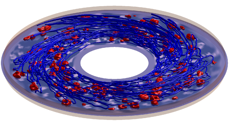
Figure 1: Field lines of the magnetic field (blue) are represented for $Rm=7000$. Both the spiral structure of the magnetic field and its quadrupolar symmetry can be identified. Isosurface corresponding to $1\%$ of the peak kinetic energy are also represented (red).

It is often assumed that the most importance source of turbulence in the interstellar medium comes from supernova explosions (McCray & Snow, 1979). The positions of these explosions are not completely random in the disk but they often occur in cluster. This produces giant expanding cavities of gas known as superbubbles. These explosions occurring in a rotating galaxy, the expansion is affected by a Coriolis force. This yields cyclonic motions and thus a strong helicity in the gas flow (Ferriere, 1998). In such a framework, however, it is worth noting that the scale separation mentioned above is not dramatic. Superbubbles have typical sizes of the order of a few hundreds parsecs (pc, see Oey & Clarke, 1997). This is smaller, but not dramatically smaller than the typical vertical scale of the galaxy ($\sim 1$ kpc). Given modern day computational resources, these numbers suggest that direct numerical simulations (i.e. numerical simulations that do not rely on an ad hoc parameterization of the small scales, for example through the $\alpha$–effect) are within reach. Indeed, (Gressel et al., 2008) recently presented such simulations. To cope with the large resolution still needed to address this problem, they adopted a local approach based on the shearing box model. Their results indicate a good agreement of the local approach with mean field models. However, the local approach they used precludes any global diagnostics, such as the global structure of the field, to be established.

The purpose of this letter is to present such global numerical simulations, resolving the magnetic field at all relevant scales in the galaxy (i.e. from $100$ parsecs to $10$ kiloparsecs). To reduce the computational burden that would be associated with full MHD simulations, we work in the kinematic regime: we solve the induction equation using a prescribed and time dependent gas flow. The later is set by using an analytical velocity field which intends to reproduce the large scale shear associated with rotation and the effect of superbubble explosions on the interstellar medium.

2 Numerical model

The direct numerical simulations presented in this letter are fully three dimensional. We solve the induction equation governing the evolution of the solenoidal magnetic field $\bf B$ in a cylindrical coordinate system $(r,\phi,z)$:

$$\frac{\partial{\bf B}}{\partial t}={\bf\nabla}\times\left({\bf u}\times{\bf B}\right)+{Rm}^{-1}\Delta{\bf B}\,,$$ (1)

written in dimensionless form using the advective timescale. The magnetic Reynolds number $Rm$ is defined as $Rm=\mu_{0}\sigma r_{0}U_{0}$, where $\mu_{0}$ is the permeability of vacuum, the typical length scale $r_{0}=10$ kpc is the radius of the galactic disk, the typical velocity scale $U_{0}$ is the velocity of the large scale flow (i.e. the differential rotation of the galaxy) and $\sigma$ is the conductivity of the plasma . In our simulations the vertical extent of the galactic disk is $H=r_{0}/10$, $z$ thus range from $-0.05r_{0}$ to $+0.05r_{0}$. We restrict our attention here to the kinematic problem, ignoring the back reaction of the magnetic field on the flow. The velocity field ${\bf u}$ used in Eq. (1) is analytical and represents the differential rotation of the galaxy and the supernova explosions. This approach also means that we do not explicitly consider important effects such as density stratification in the vertical direction or the induction effect which would be due to interstellar turbulence (Ruzmaikin et al., 1988).

Eq. (1) is solved using a finite volume approach. The method is described in details by (Teyssier et al., 2006): it uses the MUSCL–Hancok upwind method. The solenoidal character of the magnetic field ${\bf B}$ is maintained through the constrained transport algorithm (Yee, 1966; Evans & Hawley, 1988). We rely here on the so-called pseudo-vacuum boundary conditions for the magnetic field. This corresponds to imposing ${\bf B}\times{\bf n}={\bf 0}$ at all boundaries of the computational domain. These boundary conditions are not fully realistic, but they are often used in parameterized models of galactic dynamos and simple to implement. These boundary conditions are known to modify quantitative results (such as the threshold value for dynamo action) but not the global qualitative solution (Gissinger et al., 2008). We now turn to a detailed description of the velocity field being used. It is the sum of two terms: rotation around the vertical axis and modification of the flow by superbubbles. In our simulations, we use the following prescription for the rotation: ${\bf U}=U_{0}\,{\bf e}_{\Phi}$, with a constant $U_{0}$. This is a good approximation since the angular velocity is observed to be roughly proportional to $1/r$ in galaxies. The effect of supernova explosions is more subtle to implement. We decided to consider the effect of superbubbles only and ignore here isolated supernovae, as the energy input of the former is largely dominant (Ferriere, 1998). Considering superbubbles rather than smaller isolated supernovae yields larger scales which directly translates into resolutions affordable with modern days computing resources. Let us consider first the explosion of one superbubble, in a local spherical coordinate system $(r^{\prime},\theta^{\prime},\phi^{\prime})$. Following the work of (Ferriere, 1998), we work under the simplifying assumption that each explosion remnant has a perfectly spherical shape. We thus use the simple radius evolution law (Weaver et al., 1977):

$$r^{\prime}_{sb}=At^{\nu}\,,$$ (2)

During the expansion of each superbubble, the rotation of the galaxy yields a Coriolis force which tends to deflect the initially radial expansion and create cyclonic motions. This is an essential step in classical mean field $\alpha-\omega$ description of the galactic dynamo (Ferriere, 1998). This Coriolis effect can be evaluated by solving the equation of gas motion:

$$\frac{\partial{\bf v}}{\partial t}={\bf F_{e}}-2{\bf\Omega\times v_{r^{\prime}}}\,,$$ (3)

where ${\bf F_{e}}$ is a force leading to the radial expansion described by Eq. (2). Integrating Eq. (3) in the radial direction leads to the expansion (2). The azimuthal velocity is obtained by integrating the equation (3) in the azimuthal direction. In doing so, we made the approximation that the Coriolis force on the superbubble is only due to the radial expansion of the shell. Inside the superbubble, we assume a linear variation of velocity in radius. An important parameter is $r^{\prime}_{c}$, the critical size reached by the superbubble for which the pressure in the cavity becomes comparable to that of the surrounding medium. At this point, we consider that the bubble merges with the interstellar medium. This situation generally occurs when the radial velocity of the shell become comparable to the velocity of sound in the medium. In our modeling, this critical velocity numerically determines the end of existence of a superbubble. The velocity field associated with a superbubble therefore vanishes when the radial velocity reach this critical velocity $v_{c}$. This radial expansion and the associated Coriolis force totally determine the flow at small scales. In most observed galaxies, the spatial distribution of explosions in the galaxy is rapidly decreasing away from the midplane of the disk. For simplicity, we will assume here that all explosions occur in the midplane only, but with random position in the disk. In actual galaxies, there is a large observed dispersion of data about superbubbles, yet averaged values for the explosions rate of superbubbles are $f_{0}=4.5.10^{-7}$ kpc^-2yr^-1 (Elmegreen & Clemens, 1985). Such parameters, however, are still out of reach of present computations (especially because of the high explosion rate which implies large numbers of superbubbles to be handled at the same time). We use here a lower rate of superbubbles, but more powerful explosions, thus leading to a similar helicity input. In the simulations reported here, $f=f_{0}/50$, $r^{\prime}_{c}=0.4$, $A=0.35$ and $\nu=0.6$. This corresponds to about $150$ superbubbles expanding in the galactic disk at a given time in the simulations. In some cases, we will also take into account a downward flow. Due to the simplicity of our model, this velocity could be attributed to turbulent diamagnetism (Sokoloff & Shukurov, 1990) or to the galactic fountain mechanism (Shapiro & Field, 1976; Bregman, 1980). As an attempt to describe these effects, we add the following vertical velocity to the flow:

$$v_{z}(z)=\frac{-\gamma z}{\sqrt{2\pi}2\beta}\,e^{{-z^{2}}/{2\beta^{2}}}\,.$$ (4)

It is antisymmetric with respect to the midplane and vanishes for $z=0$. Moreover, the infall velocity decreases far away from the midplane. The parameter $\beta$ controls the extension of the infall region and we use here $\beta=r^{\prime}_{c}/3$ so that the maximum of the infall is near the region where superbubble explosions tend to accumulate the matter. $\gamma$ is a free parameter controlling the amplitude of the vertical velocity. We will use here $\gamma=0.03$ throughout this paper corresponding to a typical velocity of $6$ km.s^-1. Despite the simplifications implied by working in the kinematic regime, large spatial resolutions are still needed in order to correctly describe the evolution of the superbubbles at small scales. In the runs presented here, we used a resolution of $N_{r}=200$, $N_{\phi}=640$, $Nz=36$.

3 Results

3.1 General features

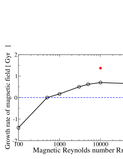
Figure 2: Growth rate of the magnetic energy as a function of the magnetic Reynolds number. Black circles correspond to simulations without infall ($\gamma=0$), whereas the filled red square corresponds to a simulation with $\gamma=0.03$.

We performed seven simulations for different magnetic Reynolds number ranging from $Rm=100$ to $Rm=10^{5}$ (this would correspond to $Rm^{\prime}$ between $0.5$ and $500$). We choose to stop the simulations after a few resistive times, when the growth rate of the magnetic energy is statistically invariant and the exponential growth is well established.

For all of these simulations, we measure the growth rate of the magnetic energy. It is displayed on figure 2 as a function of the magnetic Reynolds number $Rm$. It is negative when the magnetic Reynolds number $Rm$ is smaller than $Rm_{c}\sim 500$. It is positive for larger $Rm$, indicating exponential amplification in that case. For $Rm=10^{5}$, the growth rate is $\sigma=0.6$ Gyr^-1. Such growth rates are comparable to the ones obtained by (Gressel et al., 2008), although they seem to be larger in our case.

The result of a typical simulation ($Rm=10^{5}$) once the exponentially growing phase is reached is illustrated in figure 1 which shows simultaneously the structure of the magnetic field and that of the flow. Many superbubbles (red isosurfaces) are present at a given time in the model. We also show field lines (plotted in blue) of the magnetic field. The observed magnetic structure is the results of the combined effects of the superbubble explosions and the differential rotation of the disk. The colored slice shows the magnetic energy in the equatorial plane. It is strongly fluctuating due to the complicated nature of the flow. The overall topology of the magnetic field is complex. We now turn to a detailed study of its structure.

3.2 Structure of the magnetic field

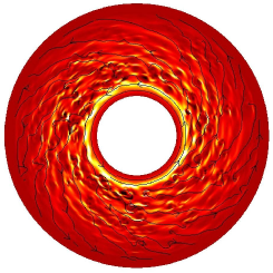
Figure 3: Structure of instantaneous magnetic field in $(r,\phi)$–plane in the midplane of the galaxy at $z=0$. Magnetic field lines projected in the $(r,\phi)$–plane are represented by black lines and the color code reflects the strength of $Bz$.

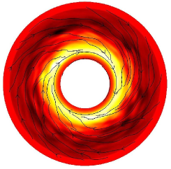
Figure 4: Magnetic field just before the top of the domain. Note that the magnetic field is smooth due to the weak effect of the superbubbles at this altitude. The sign of $B_{\phi}$ is reversed compared to the midplane.

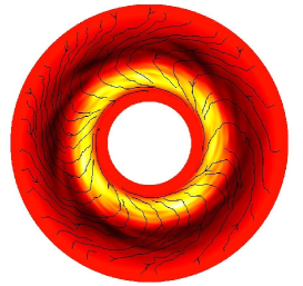
Figure 5: Magnetic field at $z=z0/2$. Note that $B_{\phi}$ change sign when the radius is increased.

a.

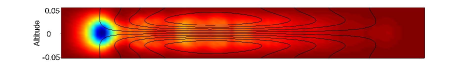
b.

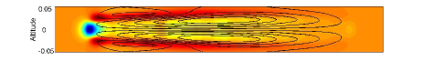
c.

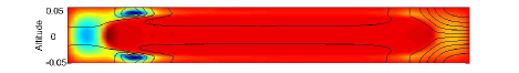
d.

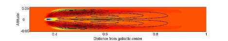
Figure 6: Magnetic structure of $\phi$-averaged magnetic field in the $(r,z)$–plane for: $Rm=1000$ (a.), $Rm=3000$ (b.) and $Rm=10^{4}$ (c. and d.). Flux expulsion is clearly visible on plot c. Plot d. corresponds to a simulation including vertical infall. Flux expulsion can thus be counteracted.

The structure in the $(r,\phi)$–plane is complicated and varies with the altitude $z$. Figure 3 shows the magnetic field in the midplane of the galaxy (the solid lines represent field lines projected in this plane and the color code indicates the strength of $Bz$).

In the midplane, the field is organized in a spiral structure. The sign of $B_{\phi}$ is constant along the radial direction. Near the axis of rotation of the disk, the azimuthal field largely dominates all others components, but rapidly goes to zero at the inner boundary in order to satisfy the boundary conditions. At larger radii, the vertical field is negligible while $B_{\phi}$ and $B_{r}$ are now comparable. Their relative value is given by the magnetic pitch angle, defined as $p_{B}={\rm atan}({B_{r}}/{B_{\phi}})$. It is remarkable that, despite the fact that numerical parameters are far from actual values, $p_{B}$ is very close to the observations: except near the unrealistic boundaries of the domain, the pitch angle is in general close to $15^{o}$, which is in agreement with the range $[-30^{o},-10^{o}]$ observed in real galaxies (Shukurov, 2007). An average of the pitch angle in radius from $r=0.2$ to $r=0.8$ gives $p_{B}\simeq-15^{o}$. This is also in agreement with (Gressel et al., 2008) although smaller, as they report a pitch angle around $10^{o}$.

At higher altitudes, the structure of the field is much more complicated. By increasing $z$, we observe that $B_{\phi}$ can change sign. We always observe opposite sign of $B_{\phi}$ between the midplane ($z=0$) and the halo ($z=+z_{0}$) (see figure 4). At intermediate altitudes, $B_{\phi}$ can also reverse sign along the radial direction itself, as it is shown in figure 5.

While the structure in the $(r,\phi)$–plane is not very sensitive to the resistivity, the magnetic field in the $(r,z)$–plane presents different behaviors depending on the value of the Reynolds number $Rm$, as shown in figure 6. A quadrupolar structure is ubiquitous in all simulations but the location of the magnetic loops does depend on $Rm$. Indeed, the effect of superbubbles is located near the midplane and produces strong expulsion of magnetic field in the halo of the galaxy. For weak $Rm$, the magnetic resistivity counteracts this effect through vertical diffusion. For larger $Rm$, the weak magnetic resistivity cannot balance anymore the strong vertical expulsion of magnetic field due to multiple explosions. As a consequence, the quadrupole becomes unrealistically confined to the halo of the galaxy (Fig. 6c), far from the active region. Although the creation of this external shell does not totally inhibit dynamo action, it clearly decreases the magnetic growth rate.

3.3 Effect of vertical infall

This behavior indicates how the diffusion of magnetic field can play two opposite roles: on the one hand, it is obviously defavorable to dynamo action by increasing resistivity in the induction equation. On the other hand, diffusion can be favorable by preventing magnetic flux expulsion away from the midplane region where the small scale flow is important. However, for weak resistivity (as is the case in real galaxies), superbubbles expel the magnetic field out of the active region of galactic disk, thus inhibiting dynamo action. In that case, adding a vertical inflow by using Eq. (4) proved to be an essential ingredient to dynamo action. This vertical flow indeed pumps the magnetic field from the halo to the midplane, which increases considerably the growth rate of magnetic energy. For $Rm=10^{4}$ for example, the growth rate increases from $\sigma=0.7$ Gy^-1 without inflow to $\sigma=1.4$ Gy^-1 with vertical inflow (filled red square on figure 2). As seen on figure 6d, the magnetic field structure is again quadrupolar in that case and is spread out over the whole galaxy.

4 Conclusion

We have shown that according to our simple model, it is possible to perform numerical simulations of the galactic dynamo without the need for a mean field formalism. We thus avoid assumptions in the scale separation and can control more rigorously the origin of the source term in the induction equation. Our simulations yield magnetic field with two main characteristics: a quadrupolar symmetry in the $(r,z)$–plane and a roughly axisymmetric spiral configuration in the $(r,\phi)$–plane. Both characteristics are in good agreement with observations and confirm previous studies that used a mean field approach. A detailed study of the magnetic field topology shows a complicated structure, with reversals of $B_{\phi}$ along the radial or vertical directions. Another interesting features of the present work are the paradoxical role of superbubbles in the limit of very weak magnetic diffusion. Indeed, the turbulent flow due to explosions is, with the differential rotation, an essential ingredient of the $\alpha-\omega$ dynamo but also inhibits dynamo action by confining the magnetic field in the halo of the galaxy. In this context, the vertical inflow of interstellar gas appears as the third main ingredient needed for dynamo action. The downward flow observed in galaxies could thus be an essential mechanism of galactic dynamo theory.

References

- Beck et al. (1996) Beck R., Brandenburg A., Moss D., Shukurov A., Sokoloff D., 1996, ARAA, 34, 155
- Bregman (1980) Bregman J. N., 1980, ApJ, 236, 577
- Elmegreen & Clemens (1985) Elmegreen B. G., Clemens C., 1985, ApJ, 294, 523
- Evans & Hawley (1988) Evans C., Hawley J., 1988, ApJ, 33, 659
- Ferriere (1992) Ferriere K., 1992, ApJ, 391, 188
- Ferriere (1998) Ferriere K., 1998, A&A, 335, 488
- Gissinger et al. (2008) Gissinger C., Iskakov A., Fauve S., Dormy E., 2008, Europhysics Letters, 82, 29001
- Gressel et al. (2008) Gressel O., Elstner D., Ziegler U., Rüdiger G., 2008, A&A, 486, L35
- Hanasz et al. (2004) Hanasz M., Kowal G., Otmianowska-Mazur K., Lesch H., 2004, ApJ, 605, L33
- Krause & Raedler (1980) Krause F., Raedler K.-H., 1980, Mean-field magnetohydrodynamics and dynamo theory. Oxford, Pergamon Press, 1980
- McCray & Snow (1979) McCray R., Snow Jr. T. P., 1979, ARAA, 17, 213
- Moffatt (1978) Moffatt H. K., 1978, Magnetic field generation in electrically conducting fluids. Cambridge, England, Cambridge University Press, 1978
- Oey & Clarke (1997) Oey M. S., Clarke C. J., 1997, MNRAS, 289, 570
- Parker (1971) Parker E. N., 1971, ApJ, 163, 255
- Rosner & Deluca (1989) Rosner R., Deluca E., 1989, in Morris M., ed., The Center of the Galaxy, IAU Symp. 136, On the Galactic Dynamo. p. 319
- Ruzmaikin et al. (1988) Ruzmaikin A. A., Sokolov D. D., Shukurov A. M., 1988, Magnetic fields of galaxies, Kluwer,Dordrecht
- Shapiro & Field (1976) Shapiro P. R., Field G. B., 1976, ApJ, 205, 762
- Shukurov (2007) Shukurov A., 2007, Galactic dynamos. Mathematical aspects of natural dynamos, Dormy, Soward (Eds) CRC Press
- Sokoloff & Shukurov (1990) Sokoloff D., Shukurov A., 1990, Nature, 347, 51
- Teyssier et al. (2006) Teyssier R., Fromang S., Dormy E., 2006, J. Comp. Phys., 218, 44
- Vainshtein & Ruzmaikin (1971) Vainshtein S. I., Ruzmaikin A. A., 1971, Astron. Zh., 48, 902
- Wang & Abel (2007) Wang P., Abel T., 2007, ArXiv e-prints 0712.0872
- Weaver et al. (1977) Weaver R., McCray R., Castor J., Shapiro P., Moore R., 1977, ApJ, 218, 377
- Wielebinski (1990) Wielebinski R., 1990, G.A.F.D., 50, 19
- Yee (1966) Yee K., 1966, IEEE Trans. Ant Prop., 14, 302