Order-invariant measures on causal sets

Abstract

A causal set is a partially ordered set on a countably infinite ground-set such that each element is above finitely many others. A natural extension of a causal set is an enumeration of its elements which respects the order.

We bring together two different classes of random processes. In one class, we are given a fixed causal set, and we consider random natural extensions of this causal set: we think of the random enumeration as being generated one point at a time. In the other class of processes, we generate a random causal set, working from the bottom up, adding one new maximal element at each stage.

Processes of both types can exhibit a property called order-invariance: if we stop the process after some fixed number of steps, then, conditioned on the structure of the causal set, every possible order of generation of its elements is equally likely.

We develop a framework for the study of order-invariance which includes both types of example: order-invariance is then a property of probability measures on a certain space. Our main result is a description of the extremal order-invariant measures.

and t1Supported in part by a grant from STICERD.

1 Introduction

This work is intended as a common generalization of two different strands of research: a proposal from physicists for a mathematical model of space–time as a discrete poset, and a notion of a “random linear extension” of an infinite partially ordered set. One of our aims is to show that these two lines of research are intimately connected.

The objects we study are causal sets, which are countably infinite partially ordered sets $P=(Z,<)$ such that every element is above only finitely many others. A natural extension of a causal set is a bijection from $\mathbb{N}$ to $Z$ whose inverse is order-preserving; that is, it is an enumeration of $Z$ that respects the ordering $<$.

We consider random processes that generate a causal set one element at a time, starting with the empty poset, and at each stage adding one new maximal element, keeping track of the order in which the elements are generated. Such a process is called a growth process. The infinite poset $P$ generated by a growth process is always a causal set, and the order in which the elements are generated is a natural extension of $P$.

We will postpone most of the formal definitions for a while, although we will introduce some notation that will be consistent with that used in the bulk of the paper. Our main purpose in this section is to motivate the ideas of the paper by examining some examples. Before that, we need a little terminology.

A (labeled) poset $P$ is a pair $(Z,<)$, where $Z$ is a set (for us, $Z$ will always be countable), and $<$ is a partial order on $Z$, that is, a transitive irreflexive relation on $Z$. An order $<$ on $Z$ is a total order or linear order if each pair $\{a,b\}$ of distinct elements of $Z$ is comparable ($a<b$ or $b<a$).

A down-set in $P$ is a subset $Y\subseteq Z$ such that, if $a\in Y$ and $b<a$, then $b\in Y$. An up-set is the complement of a down-set: a set $U\subseteq Z$ such that $b\in U$ and $a>b$ implies $a\in U$.

A pair $(x,y)$ of elements of $Z$ is a covering pair if $x<y$, and there is no $z\in Z$ with $x<z<y$. We also say that $x$ is covered by $y$, or that $y$ covers $x$.

If $P=(Z,<)$ is a poset, and $Y\subseteq Z$, then $<_{Y}$ denotes the restriction of the partial order to $Y$, and $P_{Y}=(Y,<_{Y})$. For $W\subset Z$, we also write $P\setminus W$ to mean $P_{Z\setminus W}$.

For $P=(Z,<)$ a poset on any ground-set $Z$, a linear extension of $P$ is a total order $\prec$ on $Z$ such that, whenever $x<y$, we also have $x\prec y$. In the case where $Z$ is finite, the set of linear extensions is also finite.

We will often be considering posets on the set $\mathbb{N}$, or on one of the sets $[k]=\{1,\ldots,k\}$, for $k\in\mathbb{N}$, which come equipped with a “standard” linear order. In these cases, a suborder of $\mathbb{N}$ or $[k]$ will be a partial order on that ground-set (typically denoted $<^{\mathbb{N}}$ or $<^{[k]}$) with the standard order as a linear extension, that is, if $<^{\mathbb{N}}$ is a suborder of $\mathbb{N}$ and $i<^{\mathbb{N}}j$, then $i$ is below $j$ in the standard order on $\mathbb{N}$.

In the case where the ground-set $Z$ of $P$ is countably infinite, the natural extensions of $P$ correspond to the linear extensions $\prec$ with the order-type of the natural numbers: specifically, given a natural extension of $P$, which is a bijection $\lambda\dvtx\mathbb{N}\to Z$ whose inverse is order-preserving, we obtain a linear extension $\prec$ of $P$ by setting $\lambda(i)\prec\lambda(j)$ whenever $i<j$ in the standard order on $\mathbb{N}$.

Example 1.

Figure 1 below shows the Hasse diagram of a labeled causal set $P=(Z,<)$, where $Z=\{a_{1},a_{2},\ldots\}$, and $a_{j}>a_{i}$ if $j>i+1$. (Later, we will require that the $a_{i}$ are distinct real numbers in $[0,1]$, but the order $<$ imposed on the $a_{i}$ by $P$ has no relation to the order of $[0,1]$.)

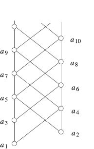
Figure 1: The causal set $P=(Z,<)$.

The natural extensions of this poset $P$ are the bijections $\lambda\dvtx\mathbb{N}\to Z$ such that, for $i<j$, $a_{i}\not>a_{j}$. Equivalently, we require that $\{\lambda(1),\ldots,\lambda(k)\}$ is a down-set in $P$, for each $k$.

We are interested in a particular probability measure $\mu$ on the set $L(P)$ of natural extensions $\lambda$ of $P$, which has properties one would associate with a “uniform” probability measure. The $\sigma$-field of measurable sets is generated by events of the form

$$E(a_{i_{1}}a_{i_{2}}\cdots a_{i_{k}})=\{\lambda\dvtx\lambda(j)=a_{i_{j}}\mbox{ for }j=1,\ldots,k\},$$

the set of natural extensions with “initial segment” $a_{i_{1}}a_{i_{2}}\cdots a_{i_{k}}$, for $k\in\mathbb{N}$ and the $i_{j}$ distinct elements of $\mathbb{N}$. We call $a_{i_{1}}a_{i_{2}}\cdots a_{i_{k}}$ an ordered stem if $\{a_{i_{1}},\ldots,a_{i_{j}}\}$ is a down-set in $P$, for $j=1,\ldots,k$: in other words if there is a natural extension of $P$ with this initial segment.

We describe the measure $\mu$ via a random process for generating the sequence $\lambda(1),\lambda(2),\ldots$ sequentially. Given the set $X_{k}=\{\lambda(1),\lambda(2),\ldots,\lambda(k)\}$, the element $\lambda(k+1)$ has to be one of the minimal elements of $P\setminus X_{k}$, and there are at most two of these. The random process we are interested in is the one defined by the following rules:

• if there is only one minimal element $a_{k}$ of $P\setminus X_{k}$, take $\lambda(k+1)=a_{k}$ with probability 1;

• if there are two minimal elements $a_{k+1}$ and $a_{k+2}$ of $P\setminus X_{k}$, set $\lambda(k+1)=a_{k+1}$ with probability $\phi=\frac{1}{2}(\sqrt{5}-1)=0.618\ldots$ and $\lambda(k+1)=a_{k+2}$ with probability $1-\phi$.

It is easy to see that the function $\lambda$ generated by these rules is always a natural extension of $P$.

We have described this as a process generating a random natural extension, but we can also think of it as a growth process, growing a causal set by adding one new maximal element at each step: the process always generates the same infinite causal set $P$, but the order in which the elements are generated is random.

We now calculate

$$\mu(E(a_{1}a_{2}))=\phi^{2}=1-\phi=\mu(E(a_{2}a_{1})).$$ (1)

Indeed, we choose $\lambda(1)=a_{1}$ with probability $\phi$; having done so, we choose $\lambda(2)=a_{2}$ with probability $\phi$. On the other hand, we choose $\lambda(1)=a_{2}$ with probability $1-\phi$; having done so, $a_{1}$ is the only minimal element of $P\setminus\{a_{2}\}$, so we choose $\lambda(2)=a_{1}$ with probability 1.

Moreover, we claim that, whenever $a_{i_{1}}a_{i_{2}}\cdots a_{i_{k}}$ and $a_{\ell_{1}}a_{\ell_{2}}\cdots a_{\ell_{k}}$ are two ordered stems with $\{a_{i_{1}},\ldots,a_{i_{k}}\}=\{a_{\ell_{1}},\ldots,a_{\ell_{k}}\}$, we have

$$\mu(E(a_{i_{1}}a_{i_{2}}\cdots a_{i_{k}}))=\mu(E(a_{\ell_{1}}a_{\ell_{2}}\cdots a_{\ell_{k}})).$$ (2)

If the two orders $a_{i_{1}}a_{i_{2}}\cdots a_{i_{k}}$ and $a_{\ell_{1}}a_{\ell_{2}}\cdots a_{\ell_{k}}$ differ only by an exchange of adjacent elements—necessarily $a_{r}$ and $a_{r+1}$ for some $r$—then (2) follows by essentially the same calculation as in (1): the two probabilities $\mu(E(a_{i_{1}}a_{i_{2}}\cdots a_{i_{k}}))$ and $\mu(E(a_{\ell_{1}}a_{\ell_{2}}\cdots a_{\ell_{k}}))$ are products of terms which are the same except that one has two terms equal to $\phi$ and the other has one term equal to $1-\phi$ and another equal to 1. To see (2) in general, it suffices to show that we can step from $a_{i_{1}}a_{i_{2}}\cdots a_{i_{k}}$ to $a_{\ell_{1}}a_{\ell_{2}}\cdots a_{\ell_{k}}$ by a sequence of exchanges of adjacent elements, staying within the set of ordered stems. This is a standard fact about the set of linear extensions of any finite poset: to see it in this case, start with the order $a_{i_{1}}a_{i_{2}}\cdots a_{i_{k}}$, and move each $a_{\ell_{j}}$ in turn down until it reaches position $j$.

The property in (2) is called order-invariance. If we consider instead a finite poset $P=(Y,<)$, then the uniform probability measure $\nu^{P}$ on the set of linear extensions of $P$ satisfies order-invariance. Indeed, another way of obtaining the measure $\mu$ in our example is to consider the sets $Z_{n}=\{a_{1},\ldots,a_{n}\}$, the finite posets $P_{n}=P_{Z_{n}}$, and the uniform measures $\nu^{P_{n}}$ on their sets of linear extensions, for each $n$. It can be shown that

$$\nu^{P_{n}}(E(a_{i_{1}}a_{i_{2}}\cdots a_{i_{k}}))\to\mu(E(a_{i_{1}}a_{i_{2}}\cdots a_{i_{k}}))$$

as $n\to\infty$, for each ordered initial segment $a_{i_{1}}a_{i_{2}}\cdots a_{i_{k}}$.

Our second example is apparently of a very different nature. We consider a family of probability measures on the set of causal sets with ground-set $\mathbb{N}$—that is, models of random causal sets—and explain how these measures also satisfy an order-invariance property.

Example 2.

A random graph order $P=(\mathbb{N},\prec)$, with parameter $p\in(0,1)$, is defined on the set $\mathbb{N}$ as follows. We take a random graph on $\mathbb{N}$—for each pair $(i,j)$ of elements of $\mathbb{N}$, we put an edge between $i$ and $j$ with probability $p$, all choices made independently. Then we define the random order $\prec$ from the random graph by declaring that $i\prec j$ if there is an increasing sequence $i=i_{1},i_{2},\ldots,i_{m}=j$ of natural numbers such that $i_{\ell}i_{\ell+1}$ is an edge for each $\ell=1,\ldots,m-1$.

Equivalently, we could define the random graph order with parameter $p$ via a growth process, adding a new maximal element at each stage. Given the restriction $P_{[k]}$ to the set $[k]$, at the next step of the process, a random subset $\Sigma$ of $[k]$ is chosen, with each element taken into $\Sigma$ independently with probability $p$. Then $k+1$ is placed above the elements of $\Sigma$, and the transitive closure is taken—so if $j$ is in $\Sigma$ and $i\preceq j$ in $P_{[k]}$, then $i$ is placed below $k+1$ in $P_{[k+1]}$.

This is a model of random posets—there are versions with the ground-set being a finite set $[n]$, or $\mathbb{Z}$—with a number of interesting features, and it also has the advantage that it is relatively easy to analyze. Accordingly, random graph orders have attracted a fair degree of attention in the combinatorics literature; see, for instance, AF , ABBJ , BB , PT .

Fix some $k\in\mathbb{N}$, and some suborder $<^{[k]}$ of $[k]$. We claim that the probability that the order $\prec_{[k]}$ on $[k]$ is equal to $<^{[k]}$ is given by

$$p^{c(<^{[k]})}(1-p)^{b(<^{[k]})},$$ (3)

where $c(<^{[k]})$ is the number of covering pairs of $([k],<^{[k]})$, and $b(<^{[k]})$ is the number of incomparable pairs.

To see this, note that, if $i$ is covered by $j$ in $<^{[k]}$, then in order for $\prec_{[k]}$ to equal $<^{[k]}$, it is necessary for $ij$ to be an edge of the random graph. Also, if $i$ and $j$ are incomparable in $<^{[k]}$, then it is necessary for $ij$ to be a non-edge. Conversely, if $i<^{[k]}j$, but $i$ is not covered by $j$, then there is some sequence $i=i_{1}i_{2}\cdots i_{m}=j$ of elements of $[k]$ such that $i_{\ell}$ is covered by $i_{\ell+1}$ in $<^{[k]}$, for $\ell=1,\ldots,m-1$. Provided that each edge $i_{\ell}i_{\ell+1}$ is in the random graph, we will have $i\prec j$ whether or not the edge $ij$ is in the random graph. Thus, $\prec_{[k]}$ is equal to $<^{[k]}$ if and only if all the covering pairs of $<^{[k]}$ span edges in the random graph, and all the incomparable pairs do not.

The key point for our purposes is that the expression (3) is an isomorphism-invariant of the poset $<^{[k]}$, and so isomorphic posets have equal probabilities of arising as $\prec_{[k]}$. We again call this property order-invariance. An interpretation is that, if we stop the process when there are $k$ elements, and look at the structure of the poset, but not at the numbering of the elements, then, conditioned on this information, each linear extension of the poset is equally likely to have been the order in which the elements were generated.

Growth processes, of a type similar to those in Example 2, were investigated by Rideout and Sorkin RS , who view them as possible discrete models for the space–time universe. The idea is that the elements of the (random) causal set form the (discrete) set of points in the space–time universe, and the partial order $\prec$ is interpreted as “is in the past light-cone of.”

The order in which the elements of the causal set are generated is not deemed to have any physical meaning, so it should not be possible to extract information about this order from the causal set at any stage. Rideout and Sorkin thus viewed growth processes as being Markov chains on the set of finite unlabeled causal sets, where each transition adds a new maximal element. They studied such processes with the property that, conditional on the causal set at some stage $k$ being equal to some unlabeled $k$-element poset $P$, each linear extension of $P$ is equally likely to have been the order in which the elements were generated. They called this property “general covariance.” Alternatively, we can view the Rideout–Sorkin processes as generating an order on the ground-set $\mathbb{N}$, as in Example 2; then the property of general covariance translates to the property of order-invariance, as described in Example 2.

In RS , Rideout and Sorkin characterized all growth processes satisfying general covariance as well as another condition called Bell causality, and also a “connectedness” condition that prevents the model breaking up as a sequence of models of posets stacked on top of one another. The models satisfying all three conditions are called classical sequential growth models or csg models; these were studied further in RS2 , Georgiou , BG . Random graph orders, as in Example 2, are the prime examples of csg models. A general csg model can be described in similar terms to our description of a random graph order as a growth model; the particular csg model is specified by a sequence of real parameters $t_{n}$ representing the relative probability of choosing the random set $\Sigma$ to be equal to a given set $S$ of size $n$.

Brightwell and Georgiou BG determined that the large-scale structure of any csg model is that of a semiorder, and in particular is quite unlike the observed space–time structure of the universe.

Varadarajan and Rideout VR and Dowker and Surya DS describe the models that can arise if the connectedness condition is dropped. Here there is a fascinating extra layer of complexity: the causal sets arising are all obtained by stacking “csg models” on top of one another, and the sizes of “later” components may depend on the detailed structure of “earlier” ones if these are finite.

The underlying reason that csg models cannot produce causal sets that resemble the observed universe seems to lie with the condition of Bell causality: it is possible to show that any process producing causal sets of the desired type (essentially, those induced on a discrete set of points arising from a Poisson process on a Lorentzian manifold) will not satisfy this condition.

Our aim in this paper is, effectively, to study the class of growth processes satisfying general covariance: this class is vastly richer than the class of csg models. For instance, if we drop the labels $a_{i}$ from the causal set in Example 1, and consider the growth process that we described there as being a process on unlabeled posets, then the property of order-invariance again translates to general covariance.

Dealing with unlabeled combinatorial structures is often awkward; in cases similar to Example 1, it is also very unnatural. So we will deal with labeled causal sets from now on, and we want to express order-invariance in terms of notation similar to that used in Example 1.

We are thus faced with the problem of how to incorporate random graph orders (and other csg models) into our setting. The numbering of the elements that we used in Example 2 specifies the order of generation of the elements, and so these numbers cannot serve as labels in the same sense as the $a_{i}$ are used to label the elements in Example 1.

It is useful at this point to introduce another family of examples, in some ways trivial but in other ways far from it.

Example 3.

We consider growth processes where the causal set generated is a.s. an antichain (i.e., no two elements are comparable). This is the case if we take a random graph order with $p=0$: we certainly do want to include some such growth processes within our framework.

If we require our causal sets to be labeled, then a growth process which a.s. generates an antichain is nothing more than a sequence of random variables: the labels of the elements, in the order they are introduced.

Order-invariance requires that, if we condition on the set of the first $k$ labels, for any $k$, then each of the $k!$ orderings of these labels is equally likely. This is exactly the requirement that the sequence of labels be exchangeable.

One way to generate a sequence of exchangeable random labels is to take any probability distribution $\tau$ on any set $X$ of potential labels, and let the labels be an i.i.d. sequence of random elements of $X$ with probability measure $\tau$. We will want our labels to be a.s. distinct, so we need the probability measure $\tau$ to be atomless.

The Hewitt–Savage theorem HS states that every sequence of exchangeable random variables is a mixture of sequences of the type described above (i.e., there is a probability measure $\rho$ on some space of probability measures on a set $X$: one measure $\tau$ is chosen according to $\rho$, and then an i.i.d. sequence of random elements of $X$ is generated according to $\tau$).

For instance, we can take $X$ to be the interval $[0,1]$, equipped with its usual Borel $\sigma$-field and Lebesgue probability measure, and $\tau$ to be the uniform probability measure on $X$. Our growth process then operates as follows: at each stage, we introduce a new element, labeled with a uniformly random element of $[0,1]$, chosen independently of all other labels, and we make the new element incomparable with all existing elements. This is indeed order-invariant: if we condition on the state of the process after $k$ steps—an antichain labeled with a set of $k$ numbers from $[0,1]$, a.s. distinct—then each of the $k!$ orders of generation is equally likely.

Formally, we will handle random graph orders in exactly the same way as in the example above: our growth process will proceed by taking a new element, assigning it a uniformly random label from $[0,1]$, independent of any other labels and of the structure of the existing poset, and then placing the new element above some of the existing elements as described in Example 2. Such a growth process will be order-invariant.

In general, it is convenient to work only with causal sets labeled by elements from a specific set, and we shall choose the interval $[0,1]$, which comes equipped with its standard (compact) topology, and the Borel $\sigma$-field $\mathcal{B}$ generated by the topology.

One generally applicable way of specifying the outcome of a growth process is by giving an infinite string of (labels of) elements, listed as $x_{1}x_{2}\cdots$ in the order of their generation, together with a suborder $<^{\mathbb{N}}$ of the index set $\mathbb{N}$ with its standard order: $i<^{\mathbb{N}}j$ if and only if $x_{i}<x_{j}$ in the causal set $P=(X,<)$ generated by the process.

Growth processes thus correspond to probability measures on the set $\Omega$ of pairs

$$(x_{1}x_{2}\cdots,<^{\mathbb{N}}),$$

where the $x_{i}$ are elements of $[0,1]$ and $<^{\mathbb{N}}$ is a suborder of $\mathbb{N}$. We will proceed by taking $\Omega$ as the outcome space, with the appropriate $\sigma$-field $\mathcal{F}$, and considering probability measures on $(\Omega,\mathcal{F})$. We will set up the notation carefully in Section 3, introducing the notion of a causal set process or causet process, which is effectively the same as a growth process, but where the states are formally pairs $(x_{1}\cdots x_{k},<^{[k]})$, where the poset $<^{[k]}$ is on the index set $[k]$, rather than on the set $X_{k}=\{x_{1},\ldots,x_{k}\}$. We give a formal definition of order-invariance, as a property of probability measures on $(\Omega,\mathcal{F})$, in Section 4.

We emphasize that we will build one space $(\Omega,\mathcal{F})$ to accommodate all causet processes, subject only to the fairly arbitrary restriction that the set of potential labels of elements is $[0,1]$. We will then study the space of all order-invariant measures, which we will define as probability measures on $(\Omega,\mathcal{F})$ satisfying a certain condition. This space of order-invariant measures has some good properties; for instance, it is a convex subset of the set of all probability measures on $(\Omega,\mathcal{F})$, and we shall show in Section 6 that it is closed in the topology of weak convergence.

In order to make a systematic study of order-invariant measures, we shall focus on the extremal order-invariant measures: those that cannot be written as a convex combination of two others.

An order-invariant measure that almost surely produces one fixed (labeled) causal set $P=(Z,<)$, as in Example 1, will be called an order-invariant measure on $P$. The process in Example 1 is in fact the only order-invariant measure on the poset $P$ of Figure 1, and it is extremal. We shall see an example later of a causal set with infinitely many extremal order-invariant measures on it.

On the other hand, it follows from the analysis in Example 3 that a labeled antichain $(Z,<)$ admits no order-invariant measures. Indeed we saw that, if an order-invariant measure generates an antichain a.s., then there is a probability measure $\rho$ on the space of probability measures on $([0,1],\mathcal{B})$, such that the sequence of labels is generated by first choosing a probability measure $\tau$ according to $\rho$, then taking an i.i.d. sequence of random variables with distribution $\tau$. Now, if $x\in[0,1]$, and $x$ occurs as a label with positive probability, then $\rho(\tau(\{x\})>0)>0$, and in that case $x$ occurs as a label infinitely often with positive probability. So such a process cannot generate each label in $Z$ exactly once.

There is however an abundance of extremal order-invariant measures that are measures on some fixed causal set. Also, there are extremal order-invariant measures a.s. giving rise to an antichain: it follows from the discussion in Example 3—in particular, from the Hewitt–Savage theorem HS —that these are effectively the same as i.i.d. sequences of random elements of $[0,1]$.

Our main result is Theorem 8.1, showing that all extremal order-invariant measures on $(\Omega,\mathcal{F})$ are, in a sense to be made precise later, a combination of extremal order-invariant measures of these two types.

Sections 2–4 are devoted to defining notation and terminology, setting up the spaces we are studying, and giving precise definitions. We also establish some useful properties of order-invariant measures in Section 4. In Section 5, we give details of how examples such as the ones in this section fit into the general framework. In Section 6, we show that the set of order-invariant measures is the set of measures invariant under a certain family of permutations on $\Omega$, and we derive as a consequence that the set of order-invariant measures is closed in the topology of weak convergence. In Section 7, we give a number of conditions equivalent to extremality of an order-invariant measure, and also show that every order-invariant measure is a mixture of extremal ones. Finally, in Section 8, we state, discuss and prove Theorem 8.1.

Our results do not provide a classification of extremal order-invariant measures: this would necessarily involve a classification of extremal order-invariant measures on fixed causal sets, which seems likely to be prohibitively difficult. However, some partial results in this direction are given in the authors’ companion paper BL2 , where order-invariant measures on fixed causal sets are studied in depth.

For now, we just point out some more connections to existing literature. Some years ago, the first author Bri1 , Bri2 studied random linear extensions of locally finite posets. The main theorem of Bri1 , interpreted in the present context, is as follows. If a causal set $P$ has the property that, for some fixed $t$, every element is incomparable with at most $t$ others, then there is a unique order-invariant measure on $P$. For instance, this applies to the causal set in Example 1. More details can be found in BL2 .

The specific case where $P$ is the two-dimensional grid $(\mathbb{N}\times\mathbb{N},<)$ has attracted considerable attention, as it is connected with the representation theory of the infinite symmetric group, and with harmonic functions on the Young lattice (which is the lattice of down-sets of $P$). A good account of this theory appears in Kerov Kerov , where a somewhat more general theory is also developed. Our concerns in this paper are different, but the two theories have various points of contact.

The family of natural extensions of a fixed causal set $P$ can also be viewed as the set of configurations of a (1-dimensional) spin system, and order-invariant measures can then be interpreted as Gibbs measures, so that some of the general results discussed in, for instance, Bovier Bovier or Georgii Georgii apply. In fact, as we shall see later, some of the results in Georgii apply to order-invariant measures in general.

2 Causal sets and natural extensions

For a poset $P=(Z,<)$ and an element $x\in Z$, set $D(x)=\{y\in Z\dvtx y<x\}$, the set of elements below $x$. We also set $U(x)=\{y\in Z\dvtx y>x\}$ and $I(x)$ to be the set of elements incomparable with $x$. Thus, $\{D(x),I(x),U(x)\}$ is a partition of $Z\setminus\{x\}$. A causal set is a poset in which $D(x)$ is finite for all $x$.

Recall that a natural extension of a causal set $P=(Z,<)$ is a bijection $\lambda$ from $\mathbb{N}$ to $Z$ such that $\lambda^{-1}$ is order-preserving: that is, if $\lambda(i)<\lambda(j)$, then $i<j$. It is often convenient to write natural extensions as $x_{1}x_{2}\cdots$, meaning that $\lambda(i)=x_{i}$. In this notation, an initial segment of $\lambda$ is an initial substring $x_{1}x_{2}\cdots x_{k}$, for some $k\in\mathbb{N}$.

A natural extension $\lambda$ of a countably infinite poset $P=(Z,<)$ gives rise to a linear extension $\prec$ of $P$ by setting $x\prec y$ whenever $\lambda^{-1}(x)<\lambda^{-1}(y)$. The linear extensions arising in this way are those with the order-type of $\mathbb{N}$.

Similarly, if $P=(Z,<)$ is a finite poset, with $|Z|=k$, we can think of a linear extension as a bijection $\lambda\dvtx[k]\to Z$ such that $\lambda^{-1}$ is order-preserving, that is, if $\lambda(i)<\lambda(j)$, then $i<j$ in $[k]$. We shall sometimes write a linear extension of a finite poset $P$ as $x_{1}\cdots x_{k}$, meaning that $\lambda(i)=x_{i}$ for $i=1,\ldots,k$. For finite partial orders, we shall use these various equivalent notions of linear extension interchangeably.

A stem in a causal set is a finite down-set (this term is less standard: it has been used in some physics papers). An ordered stem of a causal set $P=(Z,<)$ is a finite string $x_{1}\cdots x_{k}$ such that $X=\{x_{1},\ldots,x_{k}\}$ is a down-set in $P$, and $x_{1}\cdots x_{k}$ is a linear extension of $P_{X}$. In other words, ordered stems are exactly the strings that can arise as an initial segment of a natural extension of $P$.

For a countable poset $P=(Z,<)$, let $L(P)$ denote the set of natural extensions of $P$. Also, let $L^{\prime}(P)$ denote the set of injections $\lambda$ from $\mathbb{N}$ to $Z$ such that, for each $i$, $D(\lambda(i))\subseteq\{\lambda(1),\ldots,\lambda(i-1)\}$. In general, elements of $L^{\prime}(P)$ need not be bijections from $\mathbb{N}$ to $Z$: they may be invertible maps from $\mathbb{N}$ onto a proper subset of $Z$, which will necessarily be an infinite down-set in $P$. Those elements of $L^{\prime}(P)$ that are bijections from $\mathbb{N}$ to $Z$ are exactly the natural extensions of $P$.

A countable poset has a natural extension if and only if every element is above finitely many elements, that is, if and only if it is a causal set. If $P$ has no element $x$ with $I(x)$ infinite, then all linear extensions of $P$ correspond to natural extensions, and $L(P)=L^{\prime}(P)$. However, if there is an element $x$ of $P$ with $I(x)$ infinite, then there is (a) a linear extension of $P$ that does not have the order-type of $\mathbb{N}$ and (b) an element of $L^{\prime}(P)$ whose image is the proper subset $I(x)\cup D(x)$ of $P$.

3 Causal set processes

A causal set process or causet process is a discrete-time Markov chain on an underlying probability space $(\Omega,\mathcal{F},\mu)$, that we shall specify shortly. The elements of the state space $\mathcal{E}$ of the Markov chain are ordered pairs $(x_{1}\cdots x_{k},<^{[k]})$, where $x_{1}\cdots x_{k}$ is a string of elements from $[0,1]$, and $<^{[k]}$ is a suborder of $[k]$. The only permitted transitions of the chain are one-point extensions, from a pair $(x_{1}\cdots x_{k},<^{[k]})$ to a pair $(x_{1}\cdots x_{k}x_{k+1},<^{[k+1]})$, where $x_{k+1}$ is an element of $[0,1]$, and $<^{[k+1]}$ is obtained from $<^{[k]}$ by adding $k+1$ as a maximal element. A transition from the state $(x_{1}\cdots x_{k},<^{[k]})$ is thus specified by the element $x_{k+1}$ of $[0,1]$ to be appended to the string, and the set $D(k+1)$, a down-set in $([k],<^{[k]})$.

From each state $(x_{1}\cdots x_{k},<^{[k]})$, we can derive a partial order $P_{k}=(X_{k},<)$, with ground-set $X_{k}=\{x_{1},\ldots,x_{k}\}$, and $x_{i}<x_{j}$ if and only if $i<^{[k]}j$. We always interpret $<^{[k]}$ as giving a partial order $<$ on $X_{k}$ in this way. The condition that $<^{[k]}$ is a suborder of $[k]$ then translates to the condition that the linear order $x_{1}\cdots x_{k}$ is a linear extension of $P_{k}$; indeed the states of the causet process are in 1–1 correspondence with the set of pairs $(P_{k},x_{1}\cdots x_{k})$, where $P_{k}$ is a poset on $\{x_{1},\ldots,x_{k}\}$ and $x_{1}\cdots x_{k}$ is a linear extension of $P_{k}$. In this interpretation, as in Section 1, a transition adds a new maximal element, drawn from $[0,1]$, to $P_{k}$.

For fixed $k\in\mathbb{N}$, let $\mathcal{E}^{[k]}$ be the set of states $(x_{1}\cdots x_{k},<^{[k]})\in\mathcal{E}$, that is, those with $k$ elements. So all permitted transitions go from $\mathcal{E}^{[k]}$ to $\mathcal{E}^{[k+1]}$, for some $k$.

We shall declare our underlying outcome space $\Omega$ and $\sigma$-field $\mathcal{F}$ to be the simplest structure supporting all causet processes. The outcome space $\Omega$ can thus be taken to consist of all possible sequences of states, starting from the empty string. Now, each $\omega\in\Omega$ can be identified with a pair ($x_{1}x_{2}\cdots,<^{\mathbb{N}}$), where $x_{1}x_{2}\cdots$ is an infinite sequence of elements of $[0,1]$, and $<^{\mathbb{N}}$ is a suborder of $\mathbb{N}$. It is convenient for us to define $\Omega$ as the set of all such pairs $\omega=(x_{1}x_{2}\cdots,<^{\mathbb{N}})$.

We define the projections $\pi_{k}\dvtx\Omega\to\mathcal{E}^{[k]}$ by

$$\pi_{k}(x_{1}x_{2}\cdots,<^{\mathbb{N}})=\bigl{(}x_{1}\cdots x_{k},<^{\mathbb{N}}_{[k]}\bigr{)}$$

(in line with our general notation, $<^{\mathbb{N}}_{[k]}$ denotes the restriction of the order $<\mathbb{N}$ on the ground-set $\mathbb{N}$ to the subset $[k]$). In other words, $\pi_{k}$ is the “restriction” of $\omega=(x_{1}x_{2}\cdots,<^{\mathbb{N}})$ to its first $k$ entries. Thus, the sequence $\pi_{0}(\omega)$, $\pi_{1}(\omega),\ldots$ is the sequence of states corresponding to the outcome $\omega$. The map $\pi_{k}$ is then seen as the natural projection on to the $k$th state (and so in this case on to all the first $k$ states) in the sequence.

Given an element $\omega=(x_{1}x_{2}\cdots,<^{\mathbb{N}})$ of $\Omega$, we can derive a countably infinite subset $X=\{x_{1},x_{2},\ldots\}$ of $[0,1]$, together with a poset $P=(X,<)$ on $X$, where $x_{i}<x_{j}$ if and only if $i<^{\mathbb{N}}j$, and a natural extension $x_{1}x_{2}\cdots$ of $P$. Conversely, such a triple $(X,<_{P},x_{1}x_{2}\cdots)$ determines $\omega\in\Omega$ uniquely. The sequence $(P_{k})$ of finite posets can be obtained from $P$ by setting $P_{k}=P_{X_{k}}$, the restriction of $P$ to $X_{k}=\{x_{1},\ldots,x_{k}\}$, for each $k$.

We need some notation for functions on $\Omega$, that is, random elements on our probability space; where possible, for an object denoted by a Roman letter, we will use the Greek version of the letter to denote the corresponding random element. Thus, we will denote by $\xi_{k}$ the random $k$th coordinate, that is, the element in $[0,1]$ with $\xi_{k}(\omega)=\xi_{k}(x_{1}x_{2}\cdots,<^{\mathbb{N}})=x_{k}$. We shall use $\Xi_{k}$ to denote the random set $\{\xi_{1},\ldots,\xi_{k}\}$, and $\Xi$ to denote the random set $\{\xi_{1},\xi_{2},\ldots\}$. We use $\Delta_{k}$ to denote the random element taking values in the set of subsets of $[k]$ with $\Delta_{k}(\omega)=D(k)$, the down-set of elements below $k$ in $<^{\mathbb{N}}$. Finally, we will use $\prec^{\mathbb{N}}$ and $\prec^{[k]}$ to denote the partial-order valued random elements with $\prec^{\mathbb{N}}(\omega)=<^{\mathbb{N}}$ and $\prec^{[k]}(\omega)=<^{\mathbb{N}}_{[k]}$, and $\Pi$ and $\Pi_{k}$ to denote the posets induced on the random sets $\Xi$ and $\Xi_{k}$, respectively, by the random order $\prec^{\mathbb{N}}$ and $\prec^{[k]}$, respectively; in other words, $\Pi=(\Xi,\prec)$ and $\Pi_{k}=(\Xi_{k},\prec)$, where $\xi_{i}\prec\xi_{j}$ if and only if $i\prec^{\mathbb{N}}j$ or $i\prec^{[k]}j$.

Let $\mathcal{B}$ denote the family of Borel subsets of $[0,1]$. For $k\in\mathbb{N}$, sets $B_{1},\ldots,B_{k}$ in $\mathcal{B}$, and $<^{[k]}$ a partial order on $[k]$, define $(B_{1}\cdots B_{k},<^{[k]})$ to be the set of pairs $(x_{1}\cdots x_{k},<^{[k]})$ in $\mathcal{E}^{[k]}$ with $x_{i}\in B_{i}$ for each $i$. Now define

$$E\bigl{(}B_{1}\cdots B_{k},<^{[k]}\bigr{)}=\pi_{k}^{-1}\bigl{(}B_{1}\cdots B_{k},<^{[k]}\bigr{)}.$$

This subset $E(B_{1}\cdots B_{k},<^{[k]})$ of $\Omega$ is to be thought of as the event that $\xi_{i}\in B_{i}$ for $i=1,\ldots,k$, and that $\prec^{\mathbb{N}}$ has $<^{[k]}$ as its restriction to $[k]$. An event of this form will be called a basic event.

For each $k$, we now define $\mathcal{F}_{k}$ to be the $\sigma$-field generated by the sets $E(B_{1}\cdots B_{k},<^{[k]})$, and we note that $\mathcal{F}_{k}\subseteq\mathcal{F}_{k+1}$. Clearly, the family of events $E(B_{1}\cdots B_{k},<^{[k]})$ determines, and is determined by, the first $k$ states of the causet process, so the $\mathcal{F}_{k}$ form the natural filtration for our process. We then take $\mathcal{F}=\sigma(\bigcup_{k=1}^{\infty}\mathcal{F}_{k})$. A causet process thus gives rise to a probability measure $\mu$ on $\mathcal{F}$, that we will call a causet measure.

We remark that $\Omega$ can be identified formally with a subspace of the compact space $[0,1]^{\mathbb{N}}\times 2^{\mathbb{N}}$, with the product topology (and the standard topology on $[0,1]$). Here, we take an enumeration $s\dvtx\mathbb{N}\to\mathbb{N}\times\mathbb{N}$ of the set of pairs $(i,j)$ of positive integers with $i<j$, and then encode a suborder $<^{\mathbb{N}}$ of $\mathbb{N}$ as a function $q\dvtx\mathbb{N}\to\{0,1\}$ by setting $q(s^{-1}(i,j))=1$ if and only if $i<^{\mathbb{N}}j$. The topological space $[0,1]^{\mathbb{N}}\times 2^{\mathbb{N}}$ is metrisable, for instance by the metric

$$d((\mathbf{a,c}),(\mathbf{b,d}))=\sum_{i}2^{-i}(|a_{i}-b_{i}|+|c_{i}-d_{i}|).$$

The requirement that $<^{\mathbb{N}}$ be a partial order translates to: $q(s^{-1}(i,j))+q(s^{-1}(j,k))-q(s^{-1}(i,k))\leq 1$ for each $i<j<k$. The subspace of $[0,1]^{\mathbb{N}}\times 2^{\mathbb{N}}$ satisfying these constraints is therefore closed, and hence compact.

In this representation of $\Omega$ as a product space, the $\sigma$-fields $\mathcal{F}_{k}$ contain all finite-dimensional sets. By separability, every open set is a countable union of sets in $\bigcup_{k=1}^{\infty}\mathcal{F}_{k}$, so the product $\sigma$-field $\mathcal{F}$ is the Borel $\sigma$-field on $\Omega$ (see, e.g., Remark 4.A3 in Georgii or the discussion of product spaces in Chapter 3 in EK ), so our causet measures will be Borel measures. As $\Omega$ is a closed subset of a complete and separable metric space, $\Omega$ itself is also complete and separable.

As we have already indicated, we shall treat the concepts of causet measure and causet process almost interchangeably. Let us spell out why we may do this.

The family of basic events $E(B_{1}\cdots B_{k},<^{[k]})$ forms a separating class, that is, any two probability measures that agree on all basic events are equal: see, for example, Proposition 4.6 in Chapter 3 of EK or Example 1.2 in billingsley . Thus, to specify a causet measure $\mu$ on $(\Omega,\mathcal{F})$, it suffices to specify the probabilities $\mu(E(B_{1}\cdots B_{k},<^{[k]}))$ in a consistent way. Indeed, as mentioned earlier, the restriction $\mu_{k}=\mu\pi_{k}^{-1}$ of $\mu$ to $\mathcal{F}_{k}$ specifies the evolution of the process through the first $k$ steps; the measures $\mu_{k}$ are the finite-dimensional distributions of the process, and they determine the distribution of the process—see Proposition 3.2 in kallenberg or Theorem 1.1 in Chapter 4 of EK , or Example 1.2 in billingsley .

Conversely, suppose we are given the causet process as a transition function $P(\cdot,\cdot)$, that is:

• [(ii)]

• for each state $(x_{1}\cdots x_{k},<^{[k]})$ in $\mathcal{E}^{[k]}$, $P((x_{1}\cdots x_{k},<^{[k]}),\cdot)$ [the transition probability from the state $(x_{1}\cdots x_{k},<^{[k]})$] is a probability measure on $\mathcal{E}^{[k+1]}$,

• for every $k\in\mathbb{N}$, every $B_{1},\ldots,B_{k+1}\in\mathcal{B}$, and every suborder $<^{[k+1]}$ of $[k+1]$, $P(\cdot,(B_{1}\cdots B_{k+1},<^{[k+1]}))$ is a Borel-measurable function on $\mathcal{E}^{k}$.

Then the probabilities $\mu(E(B_{1}\cdots B_{k},<^{[k]}))$ can be derived as integrals of products of evaluations of the transition function. See Chapter 4 of Ethier and Kurtz EK for details.

One feature of our model that we have not built in to the space $(\Omega,\mathcal{F})$ is the requirement that the labels on elements be distinct: $\xi_{i}\not=\xi_{j}$ for each $i\not=j$. Indeed, it is convenient to include elements with repeated labels in our sample space $\Omega$, for instance, so that the space is compact. However, as we are interested in processes that generate labeled causal sets, we do demand that the transitions of a causet process are such that the probability of choosing any element more than once is 0: $\mu(\{\omega\dvtx\exists i\not=j,\xi_{i}(\omega)=\xi_{j}(\omega)\})=0$.

4 Order-invariant processes and measures

Causet processes, as defined above, are very general in nature. We are principally interested in those satisfying the property of order-invariance, which we shall define shortly.

When we consider an element $\omega=(x_{1}x_{2}\cdots,<^{\mathbb{N}})$ of $\Omega$, the real object of interest is the derived causal set $P=\Pi(\omega)$, with ground-set $X=\Xi(\omega)=\{x_{1},x_{2},\ldots\}$. Suppose that $x_{\lambda(1)}x_{\lambda(2)}\cdots$ is another natural extension of $P$; this means exactly that the permutation $\lambda$ of $\mathbb{N}$ is a natural extension of $<^{\mathbb{N}}$. There is just one suborder, which we shall denote $\lambda[<^{\mathbb{N}}]$, of $\mathbb{N}$ with the property that $(x_{\lambda(1)}x_{\lambda(2)}\cdots,\lambda[<^{\mathbb{N}}])$ induces $P$. To specify this order, note that we require $i(\lambda[<^{\mathbb{N}}])j$ if and only if $x_{\lambda(i)}<x_{\lambda(j)}$ in $P$, which is equivalent to $\lambda(i)<^{\mathbb{N}}\lambda(j)$.

Accordingly, for any $\omega=(x_{1}x_{2}\cdots,<^{\mathbb{N}})\in\Omega$, and any natural extension $\lambda$ of $<^{\mathbb{N}}$, we define the order $\lambda[<^{\mathbb{N}}]$ by: $i(\lambda[<^{\mathbb{N}}])j$ if and only if $\lambda(i)<^{\mathbb{N}}\lambda(j)$. We also define $\lambda[\omega]=(x_{\lambda(1)}x_{\lambda(2)}\cdots,\lambda[<^{\mathbb{N}}])$. As we have seen, the elements $\omega$ and $\lambda[\omega]$ of $\Omega$ give rise to the same poset $P$: in other words $\Pi(\omega)=\Pi(\lambda[\omega])$.

With this definition, the permutation $\lambda$ of $\mathbb{N}$ acts on a subset of $\Omega$. Our definition of order-invariance will demand, roughly, that, whenever $\lambda$ is a permutation of $\mathbb{N}$ that fixes all but finitely many elements, and $\lambda$ acts bijectively on a suitable subset $E$ of $\Omega$, then $\mu(\lambda[E])=\mu(E)$.

We define similar notation for the case of finite posets with ground-set $[k]$. For a permutation $\lambda$ of $[k]$, and $<^{[k]}$ a partial order on $[k]$, let $\lambda[<^{[k]}]$ be the partial order on $[k]$ given by: $i(\lambda[<^{[k]}])j$ if and only if $\lambda(i)<^{[k]}\lambda(j)$. The permutations $\lambda$ of $[k]$ such that $\lambda[<^{[k]}]$ is a suborder of $[k]$ are exactly the linear extensions of $<^{[k]}$: those where, whenever $\lambda(i)<\lambda(j)$, $i$ precedes $j$ in the standard order on $[k]$.

A measure $\mu$ on $(\Omega,\mathcal{F})$ is order-invariant if, for any finite sequence $B_{1},\ldots,\break B_{k}$ of sets in $\mathcal{B}$, any suborder $<^{[k]}$ of $[k]$, and any linear extension $\lambda$ of $<^{[k]}$, we have

$$\mu\bigl{(}E\bigl{(}B_{1}\cdots B_{k},<^{[k]}\bigr{)}\bigr{)}=\mu\bigl{(}E\bigl{(}B_{\lambda(1)}\cdots B_{\lambda(k)},\lambda\bigl{[}<^{[k]}\bigr{]}\bigr{)}\bigr{)}.$$ (4)

To check that a process or measure is order-invariant, it is enough to verify condition (4) for those $\lambda$ transposing two adjacent incomparable elements. This is a consequence of the (easy) fact that, given two linear extensions of a finite partial order, it is possible to step from one to the other via a sequence of transpositions of adjacent incomparable elements: a proof of this is sketched in Example 1.

In the case where the $B_{i}$ are singleton sets, (4) says that the probability of a state $(x_{1}\cdots x_{k},<^{[k]})$ depends only on the set $X_{k}=\{x_{1},x_{2},\ldots,x_{k}\}$ of elements, and the partial order $P_{k}$ induced on $X_{k}$ by $<^{[k]}$, and not on the order in which the elements of $X_{k}$ were generated. For instance, in Example 1, where the causet measure is prescribed by the probabilities of single states, this can be taken as the definition of order-invariance, which is exactly what we did in the Introduction. More typically, the probability of any single state $(x_{1}\cdots x_{k},<^{[k]})$ will be 0, so the definition we used in Example 1 will not suffice.

A causet process whose distribution is given by an order-invariant measure $\mu$ on $(\Omega,\mathcal{F})$ is said to be an order-invariant causet process. As we saw at the end of the previous section, we can talk about order-invariant measures and (distributions of) order-invariant processes interchangeably.

As an example, suppose $k=3$ and $<^{[k]}$ has only one related pair, $1<^{[3]}2$. Consider the linear extension $\lambda$ given by: $\lambda(1)=3$, $\lambda(2)=1$ and $\lambda(3)=2$. Then $2(\lambda[<^{[3]}])3$ is the only related pair in $\lambda[<^{[3]}]$, and this instance of the condition of order-invariance is that

$$\mu\bigl{(}E\bigl{(}ABC,<^{[3]}\bigr{)}\bigr{)}=\mu\bigl{(}E\bigl{(}CAB,\lambda\bigl{[}<^{[3]}\bigr{]}\bigr{)}\bigr{)}$$

for any $A,B,C\in\mathcal{B}$. (Think of $A$, $B$ and $C$ as disjoint for convenience.) On both sides the restriction is that the element in $A$ is below the element in $B$ in the partial order $\Pi_{3}$, while the element in $C$ is incomparable to both. The order-invariance condition tells us that, conditioned on the event “after three steps, we have an element in $A$ below an element in $B$, and an element in $C$ incomparable to both,” each possible order of generation of the three elements is equally likely. In this case, the possible orders of generation are just the ones in which the element of $A$ precedes the element in $B$: besides the two orders above, the only other possible order of generation is $ACB$. The three orders correspond to the three linear extensions of the poset $Q$ with three elements labeled $A$, $B$ and $C$, with $A$ below $B$.

Another related condition we can impose on a causet process is that transitions out of a state depend only on the set of elements generated and the partial order induced on them. Specifically, we say that a causet process (or associated measure) is order-Markov if we always have

$$\frac{\mu(E(B_{1}\cdots B_{k}B_{k+1},<^{[k+1]}))}{\mu(E(B_{1}\cdots B_{k},<^{[k]}))}=\frac{\mu(E(B_{\lambda(1)}\cdots B_{\lambda(k)}B_{k+1},\lambda^{\prime}[<^{[k+1]}]))}{\mu(E(B_{\lambda(1)}\cdots B_{\lambda(k)},\lambda[<^{[k]}]))},$$

whenever either denominator is non-zero, where $\lambda^{\prime}$ is the linear extension of $<^{[k+1]}$ derived from a linear extension $\lambda$ of $<^{[k]}$ by fixing $k+1$. We see immediately that, if a causet process is order-invariant, then it is order-Markov, as the two numerators and the two denominators above are both equal.

The converse is far from true: order-invariance is much stronger than the order-Markov condition. One way to see this is to observe that, if we impose only the order-Markov condition, then the transition laws out of states with one element need bear no relation to the transition law out of the initial “empty” state: if we demand order-invariance, then these are connected via equation (4) in cases where $<^{[2]}$ is the two-element antichain.

However, if we know that a causet process is order-Markov, then to prove order-invariance it is enough to check condition (4) for the permutation $\lambda$ exchanging the last two elements, whenever these are incomparable. To see this, let $\lambda^{(i)}$ denote the permutation of any $[k]$, with $k>i$, exchanging $i$ and $i+1$ and leaving all other elements fixed. Suppose that the causet measure $\mu$ satisfies

$$\mu\bigl{(}E\bigl{(}B_{1}\cdots B_{j-2}B_{j}B_{j-1},\lambda^{(j-1)}\bigl{[}<^{[j]}\bigr{]}\bigr{)}\bigr{)}=\mu\bigl{(}E\bigl{(}B_{1}\cdots B_{j-2}B_{j-1}B_{j},<^{[j]}\bigr{)}\bigr{)}$$

for every sequence $B_{1},\ldots,B_{j}$ of Borel sets, and every suborder $<^{[j]}$ of $[j]$ in which $j-1$ and $j$ are incomparable. Now if $\mu$ is order-Markov, we can use this condition inductively to deduce that

$$\mu\bigl{(}E\bigl{(}B_{1}\cdots B_{j-2}B_{j}B_{j-1}B_{j+1}\cdots B_{k},\lambda^{(j-1)}\bigl{[}<^{[k]}\bigr{]}\bigr{)}\bigr{)}$$

$$\qquad=\mu\bigl{(}E\bigl{(}B_{1}\cdots B_{j-2}B_{j-1}B_{j}B_{j+1}\cdots B_{k},<^{[k]}\bigr{)}\bigr{)}$$

for every $k\geq j$, every sequence $B_{1},\ldots,B_{k}$ of Borel sets, and every suborder $<^{[k]}$ of $[k]$ in which $j-1$ and $j$ are incomparable. This is exactly condition (4) for $\lambda^{(j-1)}$. As we saw earlier, we can now deduce that $\mu$ is order-invariant.

Given two probability measures $\mu_{1}$ and $\mu_{2}$ on $(\Omega,\mathcal{F})$, a convex combination of $\mu_{1}$ and $\mu_{2}$ is a probability measure of the form $r\mu_{1}+(1-r)\mu_{2}$, for $r\in(0,1)$. It is immediate from the definition that, if $\mu_{1}$ and $\mu_{2}$ are order-invariant, then so is any convex combination. Thus, the family of order-invariant measures is a convex subset of the set of all causet measures.

More generally, given a probability space $(W,\mathcal{G},\rho)$ whose elements are causet measures $\mu_{\omega}$, the mixture defined by this space is the probability measure $\mu$ defined by

$$\mu(\cdot)=\int_{W}\mu_{\omega}(\cdot)\,d\rho(\mu_{\omega}).$$

It is again immediate from the definition that, if all the $\mu_{\omega}$ are order-invariant, then so is the mixture $\mu$.

We now give an alternative characterization of order-invariance. For this, we need to introduce some notation that will feature prominently in the subsequent sections as well.

For $<^{\mathbb{N}}$ a suborder of $\mathbb{N}$, $k\in\mathbb{N}$, and $\lambda$ a linear extension of $<^{\mathbb{N}}_{[k]}$, we define $\lambda^{+}$ to be the natural extension of $<^{\mathbb{N}}$ defined by

$$\lambda^{+}(i)=\cases{\lambda(i),&\quad$i\leq k$,\cr i,&\quad$i>k$.}$$

So $\lambda^{+}[<^{\mathbb{N}}]$ is the partial order on $\mathbb{N}$ obtained from $<^{\mathbb{N}}$ obtained by permuting the first $k$ labels according to $\lambda$.

For a fixed $\omega=(x_{1}x_{2}\cdots,<^{\mathbb{N}})\in\Omega$, $k\in\mathbb{N}$, and $E\in\mathcal{F}$, we define $\nu^{k}(E)(\omega)$ as the proportion of linear extensions $\lambda$ of $<^{\mathbb{N}}_{[k]}$ such that $\lambda^{+}[\omega]$ is in $E$.

For any $\omega\in\Omega$ and $k$, the function $\nu^{k}(\cdot)(\omega)$ gives a probability measure on $\mathcal{F}$, namely the uniform measure on elements $\lambda^{+}[\omega]$ of $\Omega$, where $\lambda$ runs over linear extensions of $<^{\mathbb{N}}_{[k]}$. This measure can naturally be identified with the uniform measure on linear extensions of $\Pi_{k}(\omega)$.

Let us look more closely at $\nu^{k}(E(B_{1}\cdots B_{n},<^{[n]}))(\omega)$, where $\omega=(x_{1}x_{2}\cdots,\break<^{\mathbb{N}})$, the $B_{i}$ are Borel sets in $[0,1]$, $<^{[n]}$ is a suborder of $[n]$, and $k\leq n$. In order for this quantity to be non-zero, it is necessary for $<^{\mathbb{N}}_{[k]}$ to be isomorphic to $<^{[n]}_{[k]}$.

Suppose the poset $<^{[n]}_{[k]}$ has $\ell$ linear extensions, $\lambda_{1},\ldots,\lambda_{\ell}$. Each $\lambda_{i}$ induces a linear extension $\lambda^{\prime}_{i}$ on $<^{[n]}$, obtained by fixing the elements $k+1,\ldots,n$.

If now $\nu^{k}(E(B_{1}\cdots B_{n},<^{[n]})(\omega)$ is non-zero, then $<^{\mathbb{N}}_{[k]}$ also has $\ell$ linear extensions, and $\nu^{k}(E(B_{1}\cdots B_{n},<^{[n]}))(\omega)$ is equal to $\frac{1}{\ell}$ times the number of them that, applied to $\omega$, yield an element in $E(B_{1}\cdots B_{n},<^{[n]})$. If, for some linear extension $\rho$ of $<^{\mathbb{N}}_{[k]}$, $\rho^{+}[\omega]$ is in the set $E(B_{1}\cdots B_{n},<^{[n]})$, then we can reverse the process: for one of the linear extensions $\lambda_{i}$, $\lambda^{+}_{i}[\rho^{+}[\omega]]=\omega$. In other words, $\rho$ has to be the inverse of one of the $\lambda_{i}$, and the set of $\omega$ for which $\rho^{+}[\omega]$ is in $E(B_{1}\cdots B_{n},<^{[n]})$ is the set $E(B_{\lambda^{\prime}_{i}(1)}\cdots B_{\lambda^{\prime}_{i}(n)},\lambda^{\prime}_{i}[<^{[n]}])$.

It now follows that

$$\nu^{k}\bigl{(}E\bigl{(}B_{1}\cdots B_{n},<^{[n]}\bigr{)}\bigr{)}(\omega)=\frac{1}{\ell}\sum_{i=1}^{\ell}\mathbh{1}\bigl{(}E\bigl{(}B_{\lambda^{\prime}_{i}(1)}\cdots B_{\lambda^{\prime}_{i}(n)},\lambda^{\prime}_{i}\bigl{[}<^{[n]}\bigr{]}\bigr{)}\bigr{)}(\omega).$$ (5)

Lemma 4.1

For any $k\in\mathbb{N}$, any Borel sets $B_{1},\ldots,B_{k}$, any suborder $<^{[k]}$ of $[k]$, any linear extension $\lambda$ of $<^{[k]}$, and any $\omega\in\Omega$, we have

$$\nu^{k}\bigl{(}E\bigl{(}B_{1}\cdots B_{k},<^{[k]}\bigr{)}\bigr{)}(\omega)=\nu^{k}\bigl{(}E\bigl{(}B_{\lambda(1)}\cdots B_{\lambda(k)},\lambda\bigl{[}<^{[k]}\bigr{]}\bigr{)}\bigr{)}(\omega).$$

For $\omega=(x_{1}x_{2}\cdots,\prec^{\mathbb{N}})\in\Omega$, the quantity $\nu^{k}(E(B_{1}\cdots B_{k},<^{[k]}))(\omega)$ is the proportion of linear extensions $\rho$ of $\prec^{\mathbb{N}}_{[k]}$ such that $\rho^{+}[\omega]\in E(B_{1}\cdots B_{k},\break<^{[k]})$. We see that $\rho^{+}[\omega]\in E(B_{1}\cdots B_{k},<^{[k]})$ if and only if $(\lambda\rho)^{+}[\omega]\in\break E(B_{\lambda(1)}\times\cdots B_{\lambda(k)},\lambda[<^{[k]}])$. Therefore, as required, we have

$$\nu^{k}\bigl{(}E\bigl{(}B_{1}\cdots B_{k},<^{[k]}\bigr{)}\bigr{)}(\omega)=\nu^{k}\bigl{(}E\bigl{(}B_{\lambda(1)}\cdots B_{\lambda(k)},\lambda\bigl{[}<^{[k]}\bigr{]}\bigr{)}\bigr{)}(\omega).$$

We are now in a position to establish our alternative characterization of order-invariance.

Theorem 4.2

Let $\mu$ be a causet measure. Then $\mu$ is order-invariant if and only if

$$\mu(E)=\mathbb{E}_{\mu}\nu^{k}(E)$$

for every $E\in\mathcal{F}$ and every $k\in\mathbb{N}$.

This is an analogue of the DLR equations from statistical physics (see, e.g., Bovier Bovier ) or Section 1.2 in Georgii , about conditional probabilities. It corresponds to specifying a boundary condition outside a finite volume—here this means that we condition on all the information about $\omega$ except the order in which the first $k$ elements are generated, and then realizing the conditional Gibbs measure, which in our setting is $\nu^{k}(\cdot)(\omega)$.

Proof of Theorem 4.2 Suppose first that $\mu$ is a causet measure satisfying the condition. Consider any finite sequence $B_{1},\ldots,B_{k}$ of sets in $\mathcal{B}$, any suborder $<^{[k]}$ of $[k]$, and any linear extension $\lambda$ of $<^{[k]}$.

By Lemma 4.1, we have that

$$\nu^{k}\bigl{(}E\bigl{(}B_{1}\cdots B_{k},<^{[k]}\bigr{)}\bigr{)}(\omega)=\nu^{k}\bigl{(}E\bigl{(}B_{\lambda(1)}\cdots B_{\lambda(k)},\lambda\bigl{[}<^{[k]}\bigr{]}\bigr{)}\bigr{)}(\omega)$$

for each $\omega\in\Omega$. Taking expectations, we have

$$\mathbb{E}_{\mu}\nu^{k}\bigl{(}E\bigl{(}B_{1}\cdots B_{k},<^{[k]}\bigr{)}\bigr{)}=\mathbb{E}_{\mu}\nu^{k}\bigl{(}E\bigl{(}B_{\lambda(1)}\cdots B_{\lambda(k)},\lambda\bigl{[}<^{[k]}\bigr{]}\bigr{)}\bigr{)},$$

and therefore the given condition implies that

$$\mu\bigl{(}E\bigl{(}B_{1}\cdots B_{k},<^{[k]}\bigr{)}\bigr{)}=\mu\bigl{(}E\bigl{(}B_{\lambda(1)}\cdots B_{\lambda(k)},\lambda\bigl{[}<^{[k]}\bigr{]}\bigr{)}\bigr{)}$$

for each basic event $E(B_{1}\cdots B_{k},<^{[k]})$, as required for order-invariance.

Conversely, suppose that $\mu$ is order-invariant, and fix $k\in\mathbb{N}$. Now consider a basic event $E(B_{1}\cdots B_{n},<^{[n]})$, for $n\geq k$. Taking expectations in (5), we obtain that

$$\mathbb{E}_{\mu}\nu^{k}\bigl{(}E\bigl{(}B_{1}\cdots B_{n},<^{[n]}\bigr{)}\bigr{)}=\frac{1}{\ell}\sum_{i=1}^{\ell}\mu\bigl{(}E\bigl{(}B_{\lambda^{\prime}_{i}(1)}\cdots B_{\lambda^{\prime}_{i}(n)},\lambda^{\prime}_{i}\bigl{[}<^{[n]}\bigr{]}\bigr{)}\bigr{)},$$

where, as before, $\lambda^{\prime}_{1},\ldots,\lambda^{\prime}_{\ell}$ are the linear extensions of $<^{[n]}_{[k]}$ that fix $k+1,\ldots,n$. Now, by order-invariance, the sum above is equal to $\mu(E(B_{1}\cdots B_{n},\break<^{[n]}))$.

For each fixed $k$, we now have that $\mu(E)=\mathbb{E}_{\mu}\nu^{k}(E)$ for all the basic events $E$; as both $\mu(\cdot)$ and $\mathbb{E}_{\mu}\nu^{k}(\cdot)$ are measures, and the basic events form a separating class, we have that the condition holds for all events $E\in\mathcal{F}$.

5 Examples

In this section, we briefly revisit the three examples we introduced in Section 1, and give one more.

Causet processes on fixed causal sets

Suppose we are given a fixed causal set $P=(Z,<)$, with $Z\subset[0,1]$. Recall that $L^{\prime}(P)$ is the set of all natural extensions of posets $P_{Y}$, where $Y$ is an infinite down-set in $P$. In the case where the set $I(x)$ of elements incomparable to $x$ is finite for all $x$, $L^{\prime}(P)$ is equal to the set $L(P)$ of natural extensions of $P$.

A causet process on $P$ is a process generating a random element $\lambda$ of $L^{\prime}(P)$: we think of generating distinct elements $\lambda(1),\lambda(2),\ldots$ of $Z$ in turn. At each stage, an element $z\in Z$ is available for selection only if all the elements in $D(z)$ have already been selected [equivalently, at stage $k$, the element $z$ is available for selection if $z$ is minimal in $P\setminus\{\lambda(1),\ldots,\lambda(k-1)\}$].

We can view a causet process on $P$ as a special case of a causet process: the states that can occur are pairs $(x_{1}\cdots x_{k},<^{[k]})$, where $x_{1}\cdots x_{k}$ is an ordered stem of $P$, and $<^{[k]}$ is the poset induced from the order $<$ on $Z$: $i<^{[k]}j$ if and only if $x_{i}<x_{j}$. For a transition out of this state, at stage $k+1$, a random (not necessarily uniform) minimal element $\xi_{k+1}$ of $P\setminus\{x_{1},\ldots,x_{k}\}$ is selected, and its down-set is chosen to be the same as it is in $P$. Example 1 illustrates this.

A causet process on $P$ is order-Markov if the law describing how we choose a minimal element from $P\setminus\{x_{1},\ldots,x_{k}\}$ depends only on the set $\{x_{1},\ldots,x_{k}\}$. Again, the condition of order-invariance is much more demanding than the order-Markov condition.

One example is the process considered by Luczak and Winkler LW , which grows, step by step, uniformly random $n$-element subtrees, containing the root as the unique minimal element, of the complete $d$-ary tree $T^{d}$. This process is a causal set process on $T^{d}$, and is order-Markov, but calculations on small examples reveal that it is not order-invariant.

When considering causet processes on a fixed poset $P$, the order on any set of elements is determined by $P$, so it is natural to drop the order from the notation, and denote a state simply as $x_{1}\cdots x_{k}$, and an element $\omega$ as $x_{1}x_{2}\cdots$.

We study order-invariance on fixed causal sets in more detail in the companion paper BL2 .

We saw one example of a causet process on a fixed causal set in Example 1. As a further illustration, we give another example.

Example 4.

Let $P=(Z,<)$ be the disjoint union of two infinite chains $B\dvtx b_{1}<b_{2}<\cdots$ and $C\dvtx c_{1}<c_{2}<\cdots$, with every element of $B$ incomparable with every element of $C$. Fix a real parameter $q\in[0,1]$, and define a causet process on $P$ as follows. For any stem $A$ of $P$, there are exactly two minimal elements of $P\setminus A$, one in $B$ and one in $C$: from any state with $X_{k}=A$, we define the transition probabilities out of that state by choosing the element in $B$ with probability $q$. Denote the associated probability measure $\mu_{q}$: specifically, if $a_{1}\cdots a_{k}$ is any ordered stem of $P$ with $A=\{a_{1},\ldots,a_{k}\}=\{b_{1},\ldots,b_{m},c_{1},\ldots,c_{n}\}$, then $\mu_{q}(E(a_{1}\cdots a_{k}))=q^{m}(1-q)^{n}$. (As mentioned above, we have dropped the order $<^{[k]}$, which can be derived from $P$, from the notation.)

It follows that $\mu_{q}$ is order-invariant for any $q$, since the expression for $\mu_{q}(E(a_{1}\cdots a_{k}))$ does not depend on the order of the $a_{i}$.

The cases $q=0$ and $q=1$ are special. If $q=0$, then elements from $C$ are never chosen, and $\Xi=B$ a.s.; if $q=1$, then $\Xi=C$ a.s. If $q\in(0,1)$, then $\Xi=B\cup C=Z$ a.s.

More generally, given any probability measure $\rho$ on $[0,1]$, define a probability measure $\mu_{\rho}$ by first choosing a random parameter $\chi$ according to $\rho$, then sampling according to $\mu_{\chi}$. Then, for $a_{1}\cdots a_{k}$ is any ordered stem of $P$ with $A=\{a_{1},\ldots,a_{k}\}=\{b_{1},\ldots,b_{m},c_{1},\ldots,c_{n}\}$, we have $\mu_{\chi}(E(a_{1}\cdots a_{k}))=\mathbb{E}_{\rho}(\chi^{m}(1-\chi)^{n})$. Again, this expression is independent of the order of the $a_{i}$, so $\mu_{\rho}$ is order-invariant. (Alternatively, $\mu_{\rho}$ is a mixture of the order-invariant measures $\mu_{q}$, so is also order-invariant.)

This last description includes several apparently different processes. For instance, consider the following process: having chosen the bottom $n$ elements, $m$ from $B$ and $k=n-m$ from $C$, choose the next element to be from $B$ with probability $(m+1)/(n+2)$. It is easy to check directly that this defines an order-invariant process on $P$. The theory of Pólya’s Urn (see, e.g., Exercise E10.1 in Williams williams ) tells us that the proportion of elements taken from $B$ in the first $n$ steps converges a.s. to some limit $\chi$ as $n\to\infty$, and that this limit $\chi$ has the uniform distribution on $(0,1)$. Indeed, this process has the same finite-dimensional distributions as the one defined by choosing $\chi$ from the uniform distribution in advance, then choosing the natural extension according to $\mu_{\chi}$.

This example is covered in more detail in BL2 , and from a slightly different perspective in Kerov Kerov .

Causet processes with independent labels

Another special class of causet processes consists of those where, at every transition, the new random “label” $\xi_{k+1}$ in $[0,1]$ is chosen independently of the random down-set $\Delta_{k+1}$, and of all other labels, and where the distribution of $\Delta_{k+1}$ itself depends only on $<^{[k]}$.

In this case, the labels from $[0,1]$ play no essential role, and it is more natural to think of the elements as unlabeled, and to view a process as a Markov chain on the set of finite unlabeled causal sets. The csg models of Rideout and Sorkin RS , which include the random graph orders in Example 2, are of this type.

Let us be specific about how to realize the random graph order with parameter $p$ as an order-invariant causet process. The case $p=0$, where the random graph order is a.s. an antichain, as in Example 2, is included in this description.

From a state $(x_{1}\cdots x_{k},<^{[k]})$, we make a transition to a state $(x_{1}\cdots x_{k}x_{k+1},\break<^{[k+1]})$, where $x_{k+1}$ is chosen uniformly at random from $[0,1]$, independent of any other choices. We choose a random subset $\Sigma$ of $[k]$, with each element of $[k]$ appearing in $\Sigma$ independently with probability $p$. Now we define the down-set $D(k+1)$ to be the set of elements $i\in[k]$ with $i\leq^{[k]}j$ for some $j\in\Sigma$.

We showed in Section 1 that the probability that the random partial order $\prec_{[k]}$ is equal to a particular suborder $<^{[k]}$ of $[k]$ is given by $p^{c(<^{[k]})}(1-p)^{b(<^{[k]})}$, where $c(<^{[k]})$ is the number of covering pairs of $([k],<^{[k]})$, and $b(<^{[k]})$ is the number of incomparable pairs. Thus, for $B_{1},\ldots,B_{k}$ Borel sets in $[0,1]$, and $<^{[k]}$ a suborder of $[k]$, we have

$$\mu\bigl{(}E\bigl{(}B_{1}\cdots B_{k},<^{[k]}\bigr{)}\bigr{)}=|B_{1}|\cdots|B_{k}|p^{c(<^{[k]})}(1-p)^{b(<^{[k]})},$$

where $|\cdot|$ denotes Lebesgue measure. The product $|B_{1}|\cdots|B_{k}|$ is independent of the order of the $B_{i}$, and the quantity $p^{c(<^{[k]})}(1-p)^{b(<^{[k]})}$ is invariant under isomorphisms of the poset, so the measure $\mu$ is order-invariant.

The two special cases discussed above are, in a way, two extremes. When we have a causal set process on a fixed causal set, the label of each element determines its down-set when it is introduced: in the case of causet processes with independent labels, the label and the down-set of an element are independent.

6 Invariant measures

In this section, we develop some weaker notions of invariance, and show how these relate to order-invariance. One goal is to show that the family of order-invariant measures is a closed subset of the family of all probability measures on $(\Omega,\mathcal{F})$ with respect to the topology of weak convergence.

For $i\in\mathbb{N}$, let $\lambda^{(i)}$ be the permutation of $\mathbb{N}$ exchanging $i$ and $i+1$:

$$\lambda^{(i)}(j)=\cases{i+1,&\quad if $j=i$,\cr i,&\quad if $j=i+1$,\cr j,&\quad otherwise.}$$

For $\omega=(x_{1}x_{2}\cdots,<^{\mathbb{N}})\in\Omega$, a special case of a definition from Section 4 is that

$$\lambda^{(i)}[\omega]=\bigl{(}x_{\lambda^{(i)}(1)}x_{\lambda^{(i)}(2)}\cdots,\lambda^{(i)}[<^{\mathbb{N}}]\bigr{)}$$

whenever $\lambda^{(i)}$ is a natural extension of $<^{\mathbb{N}}$, that is, whenever $i$ and $i+1$ are incomparable in $<^{\mathbb{N}}$. We now extend $\lambda^{(i)}$ to a function $\lambda^{(i)}\dvtx\Omega\to\Omega$ by setting $\lambda^{(i)}[\omega]=\omega$ if the permutation $\lambda$ is not a natural extension of $<^{\mathbb{N}}$, that is, if $i<^{\mathbb{N}}i+1$. Note that each $\lambda^{(i)}$ is a permutation, indeed an involution, on $\Omega$.

Observe that each $\lambda^{(i)}$ is continuous with respect to the product topology on $\Omega$, and so is certainly measurable, as $\mathcal{F}$ is the Borel $\sigma$-field with respect to this topology.

For $E\in\mathcal{F}$, and $i\in\mathbb{N}$, we naturally define $\lambda^{(i)}(E)=\{\lambda^{(i)}[\omega]\dvtx\omega\in E\}$. Given also a causet measure $\mu$, we set $(\mu\circ\lambda^{(i)})(E)=\mu(\lambda^{(i)}(E))$. It is then straightforward to check that $\mu\circ\lambda^{(i)}$ is a causet measure for each $\mu$ and $i$.

Lemma 6.1

For each $i$, a causet measure $\mu$ satisfies $\mu=\mu\circ\lambda^{(i)}$ if and only if

$$\mu\bigl{(}E\bigl{(}B_{1}\cdots B_{i}B_{i+1}\cdots B_{k},<^{[k]}\bigr{)}\bigr{)}=\mu\bigl{(}E\bigl{(}B_{1}\cdots B_{i+1}B_{i}\cdots B_{k},\lambda^{(i)}\bigl{[}<^{[k]}\bigr{]}\bigr{)}\bigr{)}$$

for all $k>i$, all Borel sets $B_{1},\ldots,B_{k}$, and all suborders $<^{[k]}$ of $[k]$ such that $i$ and $i+1$ are incomparable.

The given condition amounts to saying that the two measures $\mu$ and $\mu\circ\lambda^{(i)}$ agree on all the basic events $E=E(B_{1}\cdots B_{k},<^{[k]})$ with $k>i$and $i$ and $i+1$ incomparable in $<^{[k]}$. This also holds trivially for those $<^{[k]}$ with $i<^{[k]}i+1$, so the condition is equivalent to the statement that the two measures agree on the separating class of all basic events $E=E(B_{1}\cdots B_{k},<^{[k]})$ with $k>i$.

For $k\in\mathbb{N}$, let $\Lambda^{k}=\{\lambda^{(1)},\ldots,\lambda^{(k-1)}\}$. Also, set $\Lambda=\bigcup_{k}\Lambda^{k}=\{\lambda^{(i)}\dvtx i\in\mathbb{N}\}$.

We say that a measure $\mu$ is $\Lambda^{k}$-invariant if $\mu=\mu\circ\lambda^{(i)}$ for each $\lambda^{(i)}\in\Lambda^{k}$; we say that $\mu$ is $\Lambda$-invariant if $\mu\circ\lambda^{(i)}=\mu$ for every $i$.

The following result is now immediate from Lemma 6.1.

Theorem 6.2

A measure is $\Lambda$-invariant if and only if it is order-invariant.

From Lemma 6.1, we see that a measure is $\Lambda$-invariant if and only if $\mu$ satisfies (4) whenever $\lambda$ is one of the $\lambda^{(i)}$, that is, whenever $\lambda$ exchanges two adjacent incomparable elements. As we remarked immediately after the definition of order-invariance, this special case implies that (4) holds for all $\lambda$, that is, that $\mu$ is order-invariant.

For a fixed $\omega=(x_{1}x_{2}\cdots,<^{\mathbb{N}})\in\Omega$, $k\in\mathbb{N}$, and $E\in\mathcal{F}$, recall that $\nu^{k}(E)(\omega)$ is the proportion of linear extensions $\lambda$ of $<^{\mathbb{N}}_{[k]}$ such that $\lambda^{+}[\omega]$ is in $E$.

We will now show that the measures $\nu^{k}(\cdot)(\omega)$ are $\Lambda^{k}$-invariant, a result closely related to Lemma 4.1. (To be precise, the special case of that lemma with $\lambda=\lambda^{(i)}$ and $i<k$ is also a special case of the following result, and from that special case it is easy to deduce Lemma 4.1.)

Theorem 6.3

For each $k\in\mathbb{N}$ and $\omega\in\Omega$, the measure $\nu^{k}(\cdot)(\omega)$ is $\Lambda^{k}$-invariant.

Fix $k\in\mathbb{N}$ and $\omega=(x_{1}x_{2}\cdots,\prec^{\mathbb{N}})\in\Omega$. We have to show that $\nu^{k}(E)(\omega)=\nu^{k}(\lambda^{(i)}(E))(\omega)$ for every $E\in\mathcal{F}$ and every $i<k$.

For $i<k$, we can consider $\lambda^{(i)}$ as acting on the set of linear extensions $\rho$ of $\prec^{\mathbb{N}}_{[k]}$ as follows. If $i$ and $i+1$ are incomparable in $\rho[\prec^{\mathbb{N}}_{[k]}]$—that is, if $\rho(i)$ and $\rho(i+1)$ are incomparable in $\prec^{\mathbb{N}}$—then $\lambda^{(i)}[\rho]=\lambda^{(i)}\circ\rho$; if $i$ and $i+1$ are comparable in $\rho[\prec^{\mathbb{N}}_{[k]}]$, then $\lambda^{(i)}[\rho]=\rho$. Thus, $\lambda^{(i)}$ acts as an involution on the set of linear extensions of $\prec^{\mathbb{N}}_{[k]}$.

We claim that

$$\bigl{(}\lambda^{(i)}[\rho]\bigr{)}^{+}[\omega]=\lambda^{(i)}[\rho^{+}[\omega]].$$

If $i$ and $i+1$ are comparable in $\rho[\prec^{\mathbb{N}}_{[k]}]$—that is, if $\rho(i)\prec^{\mathbb{N}}_{[k]}\rho(i+1)$—then both are equal to $\rho^{+}[\omega]$. If $i$ and $i+1$ are incomparable in $\rho[\prec^{\mathbb{N}}_{[k]}]$, then both are obtained from $\rho^{+}[\omega]=(x_{\rho^{+}(1)}x_{\rho^{+}(2)}\cdots,\rho[\prec^{\mathbb{N}}_{[k]}])$ by exchanging the terms $x_{\rho^{+}(i)}$ and $x_{\rho^{+}(i+1)}$ and changing the order to $\lambda^{(i)}[\rho[\prec^{\mathbb{N}}_{[k]}]]=(\lambda^{(i)}\circ\rho)[\prec^{\mathbb{N}}_{[k]}]$: to see that these orders are equal, note that $j<\ell$ in each order if and only if $\lambda^{(i)}\rho(j)\prec^{\mathbb{N}}_{[k]}\lambda^{(i)}\rho(\ell)$.

For a linear extension $\rho$ of $\prec^{\mathbb{N}}_{[k]}$, we see that $\rho^{+}[\omega]=(x_{\rho(1)}x_{\rho(2)}\cdots\break x_{\rho(k)}x_{k+1}\times\cdots,\rho^{+}[\prec^{\mathbb{N}}])$ is in $E$ if and only if $(\lambda^{(i)}[\rho])^{+}[\omega]=\lambda^{(i)}[\rho^{+}[\omega]]$ is in $\lambda^{(i)}(E)$.

Therefore, the proportion of linear extensions $\rho$ of $\prec^{\mathbb{N}}_{[k]}$ such that $\rho^{+}[\omega]\in E$ is the same as the proportion of linear extensions $\lambda^{(i)}[\rho]$ such that$(\lambda^{(i)}[\rho])^{+}[\omega]\!\!\in\lambda^{(i)}(E)$, and this is the desired result.

For $k\in\mathbb{N}$, define $\mathcal{G}_{k}$ to be the family of sets $H$ in $\mathcal{F}$ such that $\omega\in H$ implies $\lambda^{(i)}[\omega]\in H$ for each $i<k$. We can alternatively write

$$\mathcal{G}_{k} = \{H\in\mathcal{F}\dvtx\lambda(H)=H\mbox{ for all }\lambda\in\Lambda^{k}\}$$

$$= \{H\in\mathcal{F}\dvtx\lambda^{-1}(H)=H\mbox{ for all }\lambda\in\Lambda^{k}\};$$

that is, $\mathcal{G}_{k}$ is the family of $\Lambda^{k}$-invariant sets.

It is easy to check that each $\mathcal{G}_{k}$ is a $\sigma$-field, and also that $\mathcal{G}_{k+1}\subseteq\mathcal{G}_{k}$ for all $k$. These $\sigma$-fields $\mathcal{G}_{k}$ can be seen to correspond to the external $\sigma$-fields in Section 1.2 of Georgii .

Let

$$\mathcal{G}=\bigcap_{k=1}^{\infty}\mathcal{G}_{k}=\bigl{\{}H\in\mathcal{F}\dvtx\lambda^{(i)}(H)=H\mbox{ for all }i\bigr{\}}$$

be the tail $\sigma$-field, and call a set in $\mathcal{G}$ a tail event.

An equivalent definition of $\mathcal{G}_{k}$ is that it is the collection of sets $H\in\mathcal{F}$ such that $\omega=(x_{1}x_{2}\cdots,<^{\mathbb{N}})\in H$ implies $\lambda^{+}[\omega]\in H$ for every linear extension $\lambda$ of $<^{\mathbb{N}}_{[k]}$. To see this, note again that, if $\lambda$ is a linear extension of $<^{\mathbb{N}}_{[k]}$, then $\lambda$ can be generated from a sequence of transpositions of adjacent incomparable elements, so there is a sequence $\omega=\omega_{0},\omega_{1},\ldots,\omega_{m}=\lambda^{+}[\omega]$ of elements of $\Omega$ such that, for each $j$, $\omega_{j}=\lambda^{(i)}[\omega_{j-1}]$ for some $i<k$. If $H\in\mathcal{G}_{k}$, and $\omega\in H$, then each element of the sequence is also in $H$.

Let us now consider the effect of conditioning on the $\sigma$-field $\mathcal{G}_{k}$.

As usual, for $E\in\mathcal{F}$ and $\mathcal{H}$ a sub-$\sigma$-field of $\mathcal{F}$, we shall write $\mu(E\mid\mathcal{H})$ for the conditional expectation $\mathbb{E}_{\mu}(\mathbh{1}_{E}\mid\mathcal{H})$.

Theorem 6.4

Let $\mu$ be an order-invariant measure. For any event $E\in\mathcal{F}$, and any $k\in\mathbb{N}$, we have

$$\mu(E\mid\mathcal{G}_{k})=\nu^{k}(E)$$

almost surely.

Fix $E\in\mathcal{F}$ and $k\in\mathbb{N}$.

We start by showing that $\nu^{k}(E)(\cdot)$ is $\mathcal{G}_{k}$-measurable. Fix now $\omega=(x_{1}x_{2}\cdots,\break<^{\mathbb{N}})\in\Omega$ and $i<k$. We claim that $\nu^{k}(E)(\omega)=\nu^{k}(E)(\lambda^{(i)}[\omega])$: this will imply that $\{\omega\dvtx\nu^{k}(E)(\omega)\leq x\}$ is in $\mathcal{G}_{k}$, for all $x$, as required.

The result is immediate unless $i$ and $i+1$ are incomparable in $<^{\mathbb{N}}$, so we suppose that they are incomparable. Then, for each linear extension $\rho$ of $<^{\mathbb{N}}_{[k]}$, $\rho^{+}[\omega]$ is in $E$ if and only if the corresponding permutation $\rho\lambda^{(i)}$ of $<^{\mathbb{N}}_{[k]}$ is such that $(\rho\lambda^{(i)})[\lambda^{(i)}[\omega]]\in E$. Therefore, we indeed have $\nu^{k}(E)(\omega)=\nu^{k}(E)(\lambda^{(i)}[\omega])$.

To show that the conditional expectation $\mathbb{E}_{\mu}(\mathbh{1}_{E}\mid\mathcal{G}_{k})$ is equal to $\nu^{k}(E)$, we need to show that

$$\int_{H}\mathbh{1}_{E}\,d\mu=\int_{H}\nu^{k}(E)\,d\mu$$ (6)

for every $H\in\mathcal{G}_{k}$. The left-hand side in (6) is just $\mu(H\cap E)$.

The right-hand side is $\mathbb{E}_{\mu}(\mathbh{1}_{H}\nu^{k}(E))$. We claim that $(\mathbh{1}_{H}\nu^{k}(E))(\omega)=\nu^{k}(H\cap E)(\omega)$ for all $\omega\in\Omega$. Indeed, both sides are equal to $\nu^{k}(E)$ if $\omega\in H$, and equal to zero if not, as $H$ is an invariant set for $\Lambda_{k}$. Hence, Theorem 4.2 yields

$$\mathbb{E}_{\mu}(\mathbh{1}_{H}\nu^{k}(E))=\mathbb{E}_{\mu}\bigl{(}\nu^{k}(H\cap E)\bigr{)}=\mu(H\cap E)$$

as required.

In the terminology of Georgii , Theorem 6.4 establishes that the functions $\nu^{k}(\cdot)(\cdot)$ are a family of measure kernels, analogous to Gibbsian specifications in statistical mechanics.

Our next aim is to show that the family of order-invariant measures, and the family of $\Lambda^{k}$-invariant measures for each fixed $k$, are closed subsets of the set of all causet measures, in the topology of weak convergence.

Recall that a sequence $(\mu_{n})$ of probability measures on a space $(\Omega,\mathcal{F})$, where $\mathcal{F}$ is the Borel $\sigma$-field for some topology on $\Omega$, is said to converge weakly to a probability measure $\mu$ if $\mathbb{E}_{\mu_{n}}f\to\mathbb{E}_{\mu}f$, as $n\to\infty$, for every bounded continuous real-valued function $f$ on $\Omega$: we write $\mu_{n}\Rightarrow\mu$. There are a number of equivalent conditions—see Theorem 2.1 of Billingsley billingsley , for example. The one that we shall make use of shortly is that $\mu_{n}\Rightarrow\mu$ if and only if $\limsup\mu_{n}(F)\leq\mu(F)$ for all closed sets $F$. Another fact that we shall use later is that $\mu_{n}\Rightarrow\mu$ if and only if $\mu_{n}(E)\to\mu(E)$ for all sets $E\in\mathcal{F}$ such that $\mu(\partial E)=0$, where $\partial E$ denotes the boundary of $E$.

We have already seen that our $\sigma$-field $\mathcal{F}$ is the Borel $\sigma$-field for the product topology on $\Omega$.

Let $\mathcal{M}$ be the set of probability measures on $(\Omega,\mathcal{F})$, let $\mathcal{P}$ be the set of those measures in $\mathcal{M}$ that are order-invariant, and, for $k\in\mathbb{N}$, let $\mathcal{P}_{k}$ be the set of measures in $\mathcal{M}$ that are $\Lambda^{k}$-invariant.

Theorem 6.5

For each $i$, $\{\mu\dvtx\mu=\mu\circ\lambda^{(i)}\}$ is closed in the topology of weak convergence. As a consequence, each of the $\mathcal{P}_{k}$, and $\mathcal{P}$, are closed in the topology of weak convergence.

Suppose that $\mu_{n}\Rightarrow\mu$, and that $\mu_{n}=\mu_{n}\circ\lambda^{(i)}$ for each $n$. Let $F$ be any closed set in the product topology on $\Omega$. As $\lambda^{(i)}$ is a continuous involution, $\lambda^{(i)}(F)$ is also closed. Hence, we have $\limsup\mu^{n}(\lambda^{(i)}(F))\leq\mu(\lambda^{(i)}(F))$, or in other words $\limsup(\mu_{n}\circ\lambda^{(i)})(F)\leq(\mu\circ\lambda^{(i)})(F)$. This shows that $\mu_{n}=\mu_{n}\circ\lambda^{(i)}\Rightarrow\mu\circ\lambda^{(i)}$. (Alternatively, we could appeal to the Continuous Mapping theorem—see (2.5), or Theorem 2.7, in Billingsley billingsley .)

As weak limits are unique when they exist, we now deduce that $\mu=\mu\circ\lambda^{(i)}$.

Each of the $\mathcal{P}_{k}$, and $\mathcal{P}$, are intersections of sets of the form $\{\mu\dvtx\mu=\mu\circ\lambda^{(i)}\}$. Therefore, these too are closed in the topology of weak convergence.

7 Extremal order-invariant measures

As we mentioned in Section 4, it is immediate that any convex combination of order-invariant measures is again an order-invariant measure, so the family of all order-invariant measures is a convex subset of the set of all causet measures. As usual, an extremal order-invariant measure is one that cannot be written as a non-trivial convex combination of two others.

The family of all order-invariant measures is extremely rich. In this and the next section, our aim is to show that all the extremal members of this family are of a very special form.

Under some very general conditions, the extremal measures are exactly those that have “trivial tail;” see Bovier Bovier or Georgii Georgii , for instance. We will prove a similar result in our setting, regarding the tail $\sigma$-field $\mathcal{G}$ introduced in the previous section; it is possible to deduce this from the results in Chapter 7 of Georgii—see in particular Theorems 7.7 and 7.12 and Remark 7.13, as well as Section 7.2 therein—our proof is self-contained, and also brings in a third equivalent condition that is of special interest in our setting.

To explain this condition, we shall first show that, for each fixed $E\in\mathcal{F}$, the family $\nu^{k}(E)(\cdot)$ of random variables converges a.s. to a limit $\mathcal{G}$-measurable random measure $\nu(E)$.

Theorem 7.1

Let $\mu$ be any order-invariant measure, and let $E$ be any event in $\mathcal{F}$. Then the sequence $\nu^{k}(E)(\omega)$ converges to a $\mathcal{G}$-measurable limit $\nu(E)(\omega)$ $\mu$-a.s. Moreover, $\nu(E)=\mu(E\mid\mathcal{G})$, $\mu$-a.s., and $\mathbb{E}_{\mu}\nu(E)=\mu(E)$.

Firstly, as $\mathcal{G}_{1}\supseteq\mathcal{G}_{2}\supseteq\cdots,$ the sequence $\mu(E\mid\mathcal{G}_{k})=\mathbb{E}_{\mu}(\mathbh{1}_{E}\mid\mathcal{G}_{k})$ forms a backward martingale with respect to the sequence $(\mathcal{G}_{k})$, for any $E\in\mathcal{F}$. Therefore, by the Backward Martingale Convergence theorem (see, e.g., Grimmett and Stirzaker GrSt ), $\mu(E\mid\mathcal{G}_{k})=\nu^{k}(E)$ converges a.s. to some random variable $\nu(E)$. Given $n\in\mathbb{N}$, $\nu^{k}(E)$ is $\mathcal{G}_{n}$-measurable for $k\geq n$, and hence so is $\nu(E)$; therefore, the limit $\nu(E)$ is $\mathcal{G}$-measurable.

To show that $\nu(E)=\mu(E\mid\mathcal{G})$ a.s., we need to verify that, for all $H\in\mathcal{G}$,

$$\mathbb{E}_{\mu}(\mathbh{1}_{H\cap E})=\mathbb{E}_{\mu}(\mathbh{1}_{H}\nu(E)).$$ (7)

By (6), we have that

$$\mathbb{E}_{\mu}(\mathbh{1}_{H\cap E})=\mathbb{E}_{\mu}(\mathbh{1}_{H}\nu^{k}(E))$$

for every $H\in\mathcal{G}$ and every positive integer $k$. By almost sure and bounded convergence, the right-hand side of the last equation tends to $\mathbb{E}_{\mu}(\mathbh{1}_{H}\nu(E))$ as $k\to\infty$, as required.

The result that $\mathbb{E}_{\mu}\nu(E)=\mu(E)$ is the special case of (7) with $H=\Omega$.

We say that an order-invariant measure $\mu$ is essential if, for every $E\in\mathcal{F}$, $\nu^{k}(E)\to\mu(E)$ a.s. In other words, $\mu$ is essential if, for every $E$, the limit $\nu(E)$ in Theorem 7.1 is a.s. equal to $\mu(E)$, or equivalently $\mu(E\mid\mathcal{G})=\mu(E)$ a.s.

We say that $\mu$ has trivial tails if $\mu(H)$ is equal to 0 or 1 for every $H\in\mathcal{G}$. As usual, this is equivalent to saying that every $\mathcal{G}$-measurable random variable is constant. We now establish two alternative characterizations of extremal order-invariant measures.

Theorem 7.2

The following are equivalent for an order-invariant measure $\mu$: [(iii)]

$\mu$ is extremal;

$\mu$ has trivial tails;

$\mu$ is essential.

We will show that (ii) $\Rightarrow$ (iii) $\Rightarrow$ (i) $\Rightarrow$ (ii).

(ii) $\Rightarrow$ (iii). If $\mu$ has trivial tails, then, for any $E\in\mathcal{F}$, the $\mathcal{G}$-measurable random variable $\nu(E)=\mu(E\mid\mathcal{G})$ is a.s. constant. As $\nu(E)$ is bounded, it is a.s. equal to its expectation $\mu(E)$. Thus, $\mu$ is essential.

(iii) $\Rightarrow$ (i). Suppose $\mu$ is essential; we aim to show it is extremal.

If $\mu$ is not extremal, then we can write $\mu=\alpha\mu_{0}+(1-\alpha)\mu_{1}$ for two distinct order-invariant measures $\mu_{0},\mu_{1}$ and some $\alpha\in(0,1)$.

As $\mu_{0}\not=\mu$, we may choose some $E\in\mathcal{F}$ such that $\mu_{0}(E)<\mu(E)$.

Applying Theorem 7.1 to $\mu_{0}$, for this event $E$, we obtain that there is a limiting random variable $\nu_{0}(E)$, such that $\mathbb{E}_{\mu_{0}}(\nu_{0}(E))=\mu_{0}(E)$ and $\nu^{k}(E)\to\nu_{0}(E)$, $\mu_{0}$-a.s.

Then $\mu_{0}(E)=\mathbb{E}_{\mu_{0}}(\nu_{0}(E))\geq\mu(E)\mu_{0}(\{\omega\dvtx\nu_{0}(E)(\omega)\geq\mu(E)\})$, so

$$\mu_{0}\bigl{(}\{\omega\dvtx\nu_{0}(E)(\omega)\geq\mu(E)\}\bigr{)}\leq\frac{\mu_{0}(E)}{\mu(E)}<1,$$

which implies that $\mu_{0}(\{\omega\dvtx\nu^{k}(E)(\omega)\to\mu(E)\})<1$, and so $\mu(\{\omega\dvtx\nu^{k}(E)(\omega)\to\mu(E)\})<1$. Thus, $\mu$ is not essential.

(i) $\Rightarrow$ (ii). Suppose $\mu$ does not have trivial tails, and take some tail event $H\in\mathcal{G}$ with $0<\mu(H)<1$.

We now consider conditioning $\mu$ on the occurrence or not of $H$. Let $\mu_{1}(E)=\mu(E\cap H)/\mu(H)$, and $\mu_{0}(E)=\mu(E\cap H^{c})/\mu(H^{c})$, where $H^{c}$ is the complement of $H$, for every $E\in\mathcal{F}$. Then certainly $\mu=\mu(H)\mu_{1}+(1-\mu(H))\mu_{0}$, and $\mu_{1}\not=\mu_{0}$. It remains to verify that $\mu_{1}$ and $\mu_{0}$ are order-invariant: this will imply that $\mu$ is a convex combination of two distinct order-invariant measures, so is not extremal.

It will suffice to consider $\mu_{1}$. We have to show that

$$\mu\bigl{(}E\bigl{(}B_{1}\cdots B_{k},<^{[k]}\bigr{)}\cap H\bigr{)}=\mu\bigl{(}E\bigl{(}B_{\lambda(1)}\cdots B_{\lambda(k)},\lambda\bigl{[}<^{[k]}\bigr{]}\bigr{)}\cap H\bigr{)},$$

whenever $B_{1},\ldots,B_{k}$ are Borel sets, and $\lambda$ is a linear extension of $<^{[k]}$.

By Theorem 6.4, since $H\in\mathcal{G}_{k}$ we have

$$\mu\bigl{(}E\bigl{(}B_{1}\cdots B_{k},<^{[k]}\bigr{)}\cap H\bigr{)} = \int_{H}\mathbh{1}_{E(B_{1}\cdots B_{k},<^{[k]})}\,d\mu(\omega)$$

$$= \int_{H}\nu^{k}\bigl{(}E\bigl{(}B_{1}\cdots B_{k},<^{[k]}\bigr{)}\bigr{)}(\omega)\,d\mu(\omega).$$

Lemma 4.1 tells us that

$$\nu^{k}\bigl{(}E\bigl{(}B_{1}\cdots B_{k},<^{[k]}\bigr{)}\bigr{)}(\omega)=\nu^{k}\bigl{(}E\bigl{(}B_{\lambda(1)}\cdots B_{\lambda(k)},\lambda\bigl{[}<^{[k]}\bigr{]}\bigr{)}\bigr{)}(\omega)$$

for all $\omega$; integrating over $H$ now implies that

$$\int_{H}\nu^{k}\bigl{(}E\bigl{(}B_{1}\cdots B_{k},<^{[k]}\bigr{)}\bigr{)}(\omega)\,d\mu(\omega)$$

$$\qquad=\int_{H}\nu^{k}\bigl{(}E\bigl{(}B_{\lambda(1)}\cdots B_{\lambda(k)},\lambda\bigl{[}<^{[k]}\bigr{]}\bigr{)}\bigr{)}(\omega)\,d\mu(\omega)$$

$$\qquad=\mu\bigl{(}\bigl{(}E\bigl{(}B_{\lambda(1)}\cdots B_{\lambda(k)},\lambda\bigl{[}<^{[k]}\bigr{]}\bigr{)}\bigr{)}\cap H\bigr{)}$$

again by Theorem 6.4, which completes the proof.

Our next result is somewhat related to Theorems 7.1 and 7.2: we show that, for any order-invariant measure $\mu$, for $\mu$-a.e. $\omega$, the sequence $\nu^{k}(\cdot)(\omega)$ of measures converges weakly to a version of $\mu(\cdot\mid\mathcal{G})(\omega)$; in particular, if $\mu$ is extremal, then, $\mu$-a.s., the $\nu^{k}(\cdot)(\cdot)$ converge weakly to $\mu(\cdot)$. Although this is superficially similar to the result that extremal order-invariant measures are essential, the consequences are actually rather different. Our proof is closely related to that of Proposition 7.25 in Georgii Georgii .

Theorem 7.3

There is a family $[\hat{\nu}(\cdot)(\omega)]_{\omega\in\Omega}$ of order-invariant probability measures on $(\Omega,\mathcal{F})$ such that, for any order-invariant measure $\mu$ on $\mathcal{F}$, and $\mu$-almost every $\omega$,

$$\nu^{k}(\cdot)(\omega)\Rightarrow\hat{\nu}(\cdot)(\omega).$$

Moreover, for each fixed $E\in\mathcal{F}$, and each order-invariant measure $\mu$,

$$\hat{\nu}(E)(\omega)=\mu(E\mid\mathcal{G})(\omega)=\nu(E)(\omega),\qquad\mu\mbox{-a.s.}$$

Since $(\Omega,\mathcal{F})$ is Borel, and complete and separable with respect to the product topology discussed in Section 3, it is thus standard Borel in the terminology of Georgii Georgii . Then by Theorem (4.A11) in Georgii , $(\Omega,\mathcal{F})$ has a countable core $\mathcal{C}$, that is, a countable collection of sets in $\mathcal{F}$ with the following properties: [(ii)]

$\mathcal{C}$ generates $\mathcal{F}$, and is a $\pi$-system,

whenever $(\nu^{k})$ is a sequence of probability measures such that $\nu^{k}(E)$ converges for all $E\in\mathcal{C}$, then there is a (unique) probability measure $\hat{\nu}$ on $(\Omega,\mathcal{F})$ such that $\hat{\nu}(E)=\lim_{k\to\infty}\nu^{k}(E)$ for all $E\in\mathcal{C}$.

Let $\mathcal{C}$ be a countable core in $\mathcal{F}$, and let

$$\Omega_{0}=\{\omega\in\Omega\dvtx\nu^{k}(E)(\omega)\mbox{ converges }\forall E\in\mathcal{C}\}.$$

For $\omega\in\Omega_{0}$ and $E\in\mathcal{C}$, the limit $\lim_{k\to\infty}\nu^{k}(E)(\omega)$ is equal to the $\mathcal{G}$-measurable function $\nu(E)(\omega)$, as defined in Theorem 7.1: that result tells us that $\mu(\Omega_{0})=1$ for any order-invariant measure $\mu$. We also note that $\Omega_{0}\in\mathcal{F}$, as the $\nu^{k}(E)$ are $\mathcal{F}$-measurable, and the statement that $(\nu^{k}(E)(\omega))$ is a Cauchy sequence can be written in terms of these functions. Moreover, $\Omega_{0}\in\mathcal{G}_{k}$ for all $k$, as $\nu^{n}(E)$ is $\mathcal{G}_{k}$-measurable for $n\geq k$, and so $\Omega_{0}\in\mathcal{G}$.

For each $\omega\in\Omega_{0}$, the $\nu^{k}(\cdot)(\omega)$ are probability measures, and therefore, since $\mathcal{C}$ is a core, the family $\nu(E)(\omega)$ ($E\in\mathcal{C}$) may be extended uniquely to a probability measure $\hat{\nu}(\cdot)(\omega)$ on $(\Omega,\mathcal{F})$.

For convenience, we fix one order-invariant measure $\nu_{0}$, and set $\hat{\nu}(\cdot)(\omega)=\nu_{0}(\cdot)$ for $\omega\notin\Omega_{0}$.

We next claim that, for each fixed $E\in\mathcal{F}$, and any order-invariant measure $\mu$, $\hat{\nu}(E)$ is a version of $\mu(E\mid\mathcal{G})$.

Let $\mathcal{D}=\{E\in\mathcal{F}\dvtx\hat{\nu}(E)\mbox{ is $\mathcal{G}$-measurable}\}$. The family $\mathcal{D}$ contains the countable core $\mathcal{C}$, since $\hat{\nu}(E)$ coincides with $\nu(E)$ for $E\in\mathcal{C}$—except on the $\mathcal{G}$-measurable set $\overline{\Omega_{0}}$, on which it is constant—and we saw in Theorem 7.1 that $\nu(E)(\cdot)$ is $\mathcal{G}$-measurable. We also see that $\mathcal{D}$ is a Dynkin-system (see, e.g., Williams williams ), that is, it is closed under relative complementation and increasing countable unions. By Dynkin’s $\pi$-$\lambda$ theorem (see williams , Theorem A1.3), $\mathcal{D}$ contains the $\sigma$-field generated by $\mathcal{C}$, which is $\mathcal{F}$. Therefore, $\hat{\nu}(E)$ is $\mathcal{G}$-measurable for all $E\in\mathcal{F}$.

We now need to show that, for any order-invariant measure $\mu$,

$$\int_{H}\hat{\nu}(E)\,d\mu=\int_{H}\mathbh{1}_{E}\,d\mu$$

for all $H\in\mathcal{G}$ and $E\in\mathcal{F}$. This is satisfied if $\mu(H)=0$. For other $H$, we can divide by $\mu(H)$ and express the required identity as

$$\frac{\mathbb{E}_{\mu}(\mathbh{1}_{H}\hat{\nu}(E))}{\mu(H)}=\frac{\mu(E\cap H)}{\mu(H)}$$

for all $E\in\mathcal{F}$. We see that both sides of the above identity are probability measures on $(\Omega,\mathcal{F})$: the left-hand side is countably additive, and equal to 1 for $E=\Omega$, since $\hat{\nu}$ is a probability measure, while the right-hand side is the probability measure conditional on $H$. Moreover the two measures agree on $\mathcal{C}$, as we established in Theorem 7.1. Since $\mathcal{C}$ is a $\pi$-system generating $\mathcal{F}$, this implies that the two measures are equal (see, e.g., Lemma 1.6 in Williams williams ).

Thus, for each fixed $E\in\mathcal{F}$, and each order-invariant measure $\mu$, $\hat{\nu}(E)$ is indeed a version of $\mu(E\mid\mathcal{G})$.

Combining this with Theorem 7.1 tells us that, for each $E\in\mathcal{F}$, and each order-invariant measure $\mu$,

$$\hat{\nu}(E)(\omega)=\mu(E\mid\mathcal{G})(\omega)=\nu(E)(\omega)=\lim_{k\to\infty}\nu^{k}(E)(\omega),\qquad\mu\mbox{-a.s.}$$ (8)

Now let $\tilde{\mathcal{C}}$ be the family of events of the form $E(B_{1}\cdots B_{n},<^{[n]})$, where the $B_{i}$ are open intervals in $[0,1]$ with rational endpoints in $[0,1]$ (including half-open intervals with endpoints 0 or 1). Note that $\tilde{\mathcal{C}}$ is a countable family, and a basis for the product topology on $\Omega$. Further, $\tilde{\mathcal{C}}$ is a $\pi$-system. By Theorem 2.2 in Billingsley billingsley (see also Examples 1.2 and 2.4 therein), for weak convergence of a sequence of probability measures to a probability measure, it is enough to verify convergence on the sets in $\tilde{\mathcal{C}}$. Let

$${\tilde{\Omega}}_{0}=\{\omega\in\Omega_{0}\dvtx\nu^{k}(E)(\omega)\to\hat{\nu}(E)(\omega)\mbox{ }\forall E\in\tilde{\mathcal{C}}\}.$$

By (8) and the choice of $\tilde{\mathcal{C}}$ to be countable, we have that $\mu({\tilde{\Omega}}_{0})=1$, for any order-invariant measure $\mu$.

Now, for $\omega\in{\tilde{\Omega}}_{0}$, since $\hat{\nu}(\cdot)(\omega)$ and all of the $\nu^{k}(\cdot)(\omega)$ are probability measures, and $\nu^{k}(E)(\omega)\to\hat{\nu}(E)(\omega)$ for all $E\in\tilde{\mathcal{C}}$, we deduce that $\nu^{k}(\cdot)(\omega)\Rightarrow\hat{\nu}(\cdot)(\omega)$.

For each fixed $\ell$, all the measures $\nu^{k}(\cdot)(\omega)$ for $k\geq\ell$ are $\Lambda^{\ell}$-invariant, by Theorem 6.3. By Theorem 6.5, it follows that, for $\omega\in{\tilde{\Omega}}_{0}$, the weak limit $\hat{\nu}(\cdot)(\omega)$ is $\Lambda^{\ell}$-invariant for each $\ell$, and so is order-invariant.

Using this result, we obtain a fourth equivalent condition for an order-invariant measure $\mu$ to be extremal. This condition is a weak version of the property of being essential, which can be easier to check, as we shall see shortly.

Corollary 7.4

Let $\mathcal{H}$ be the family of basic events $E=E(B_{1}\cdots B_{n},\break<^{[n]})$ where each $B_{i}$ is a closed interval with rational endpoints. Suppose that $\mu$ is an order-invariant measure such that, for each $E\in\mathcal{H}$, $\nu^{k}(E)\to\mu(E)$ a.s. Then $\mu$ is essential, and therefore extremal.

The property we need of $\mathcal{H}$ is that it is a countable separating class.

Let $[\hat{\nu}(\cdot)(\omega)]_{\omega\in\Omega}$ be the family of order-invariant measures guaranteed by Theorem 7.3. For each $E\in\mathcal{H}$, we have that $\hat{\nu}(E)(\omega)=\nu(E)(\omega)=\mu(E)$ for $\mu$-almost every $\omega$. As $\mathcal{H}$ is countable, this implies that, a.s., $\hat{\nu}(E)=\mu(E)$ for all $E\in\mathcal{H}$. Since $\mathcal{H}$ is a separating class, and $\hat{\nu}$ and $\mu$ are both measures, this implies that $\hat{\nu}=\mu$ a.s. Now, for any $E\in\mathcal{F}$, an application of Theorem 7.3 gives that $\nu(E)=\hat{\nu}(E)=\mu(E)$ a.s., so $\mu$ is essential, as claimed.

To illustrate some of the subtleties involved here, we consider processes where the partial order $<^{\mathbb{N}}$ generated is a.s. an antichain, as in Example 3. Fix any element $\omega=(x_{1}x_{2}\cdots,<^{\mathbb{N}})$ of $\Omega$, where $<^{\mathbb{N}}$ is the antichain on $\mathbb{N}$, and $x_{1},x_{2},\ldots$ is a sequence of distinct elements of $[0,1]$.

For a Borel subset $B$, $E(B)=E(B,<^{\mathbb{N}}_{[1]})$ is the event that the first element is in $B$. Now, for any $k$, $\nu^{k}(E(B))(\omega)$ is the proportion of the elements $x_{1},\ldots,x_{k}$ that lie in $B$. So $\nu^{k}(E(\{x_{j}\}))(\omega)=1/k\to 0$ as $k\to\infty$, for each fixed $j$, yet $\nu^{k}(E(\{x_{1},x_{2},\ldots\}))(\omega)=1$ for all $k$.

So, if we have a process that generates an antichain a.s., then we can never have a measure $\hat{\nu}$ such that $\nu^{k}(E)(\omega)\to\hat{\nu}(E)$ for every set $E\in\mathcal{F}$. However, such sequences $\nu^{k}(\cdot)(\omega)$ may have weak limits. Indeed, weak convergence to a measure $\hat{\nu}$ only guarantees convergence on $\hat{\nu}$-continuity sets $E$, that is, sets $E$ whose boundary $\partial E$ satisfies $\hat{\nu}(\partial E)=0$.

To be specific, consider the process that assigns independent uniform labels from $[0,1]$ to the elements as they are generated. Then, for any Borel subset $B$ of $[0,1]$, $\nu^{k}(E(B))$ is the proportion of elements of $B$ among $X_{k}=\{x_{1},\ldots,x_{k}\}$, and, by the strong law of large numbers, $\nu^{k}(E(B))\to|B|$ a.s., where $|\cdot|$ denotes Lebesgue measure. Similarly, for $k\geq n$ and $<^{[n]}$ the antichain on $[n]$, $\nu^{k}(E(B_{1}\cdots B_{n},<^{[n]}))$ is the proportion of $n$-tuples of distinct elements $(x_{i_{1}},\ldots,x_{i_{n}})$ from the set $X_{k}$ such that $x_{i_{j}}\in B_{j}$ for each $j=1,\ldots,n$. This proportion tends to $|B_{1}|\cdots|B_{n}|$ a.s. (and the limit is equal to 0 if $<^{[n]}$ is not the antichain). The sequence $\nu^{k}(\cdot)$ thus a.s. converges weakly to the product Lebesgue measure on $[0,1]^{\mathbb{N}}$. The process described here is essential, and therefore extremal, by Corollary 7.4.

This phenomenon can also be seen in otherwise well-behaved examples. For instance, in Example 1, where we have an order-invariant measure on the fixed causal set $P$, let $\omega=(a_{1}a_{2}\cdots)$—as before, the order is implied—and let $E$ be the event $\{\omega=(x_{1}x_{2}\cdots)\in\Omega\dvtx x_{i}=a_{i}\mbox{ for all but finitely many }i\}$. Then $\nu^{k}(E)(\omega)=1$ for all $k$; however $\nu^{k}(\cdot)(\omega)\Rightarrow\mu$, and $\mu(E)=0$.

In Theorems 7.1 and 7.3, we showed that, for each fixed $E\in\mathcal{F}$, and any order-invariant measure $\mu$, $\nu^{k}(E)(\omega)$ tends $\mu$-a.s. to $\hat{\nu}(E)(\omega)$, where $\hat{\nu}(\cdot)(\omega)$ is $\mu$-a.s. an order-invariant measure. We will now show that the measures $\hat{\nu}(\cdot)(\omega)$ are $\mu$-a.s. extremal; it will follow that an order-invariant measure $\mu$ can be decomposed uniquely as a mixture of these extremal order-invariant measures.

Similar results are proved in Chapter 7 of Georgii Georgii . Instead of using these results, we shall apply a result of Berti and Rigo berti-rigo giving a “conditional 0–1 law.”

The function taking $\omega\in\Omega$ to $\hat{\nu}(\cdot)(\omega)$ is a regular conditional distribution for any order-invariant measure $\mu$ given $\mathcal{G}$: that is, each $\hat{\nu}(\cdot)(\omega)$ is a probability measure, and that $\hat{\nu}(E)=\mu(E\mid\mathcal{G})$ $\mu$-a.s., for all $E\in\mathcal{F}$—which we showed in Theorem 7.3. Moreover, as $\hat{\nu}(E)(\omega)$ is independent of the particular order-invariant measure $\mu$, the tail $\sigma$-field $\mathcal{G}$ is sufficient for the collection $\mathcal{P}$ of order-invariant measures.

The following result is (essentially) Lemma 5 of berti-rigo , which in turn is adapted from a result of Maitra maitra .

Lemma 7.5 ((Berti–Rigo))

Let $\mathcal{F}$ be a countably-generated $\sigma$-field of subsets of a set $\Omega$. Let $\Lambda$ be a countable set of $\mathcal{F}$-measurable functions, and let $\mathcal{P}$ be the family of $\Lambda$-invariant probability measures on $(\Omega,\mathcal{F})$. Let $\mathcal{G}$ be a sub-$\sigma$-field of $\mathcal{F}$ that is sufficient for $\mathcal{P}$, and let $\hat{\nu}(\cdot)(\cdot)$ be a regular conditional distribution for all $\mu\in\mathcal{P}$ given $\mathcal{G}$.

Then, for any $\mu\in\mathcal{P}$, there is a set $G\in\mathcal{G}$ with $\mu(G)=1$ such that $\hat{\nu}(H)(\omega)\in\{0,1\}$ for all $H\in\mathcal{G}$ and $\omega\in G$.

Evidently all the conditions of this lemma are satisfied in our setting, and so the conclusion holds: it says that the probability measure $\hat{\nu}(\cdot)(\omega)$ is tail-trivial, for $\mu$-almost every $\omega$.

We now show that every order-invariant measure can be written uniquely as a mixture of extremal order-invariant measures.

Corollary 7.6

For any order-invariant measure $\mu$, there is a family $[\tilde{\nu}(\cdot)(\omega)]_{\omega\in\Omega}$ of extremal order-invariant probability measures on $(\Omega,\mathcal{F})$, with $\tilde{\nu}=\hat{\nu}$, $\mu$-a.s., such that $\mu$ can be decomposed as

$$\mu(\cdot)=\int\tilde{\nu}(\cdot)(\omega)\,d\mu(\omega).$$ (9)

Moreover, this is the unique decomposition of $\mu$ as a mixture of extremal order-invariant measures, up to a.s.

Given an order-invariant measure $\mu$, let $G\in\mathcal{G}$ be the set guaranteed in Lemma 7.5, with $\mu(G)=1$ and $\hat{\nu}(H)(\omega)\in\{0,1\}$ for all $H\in\mathcal{G}$ and $\omega\in G$. For $\omega\in G$, $\hat{\nu}(\cdot)(\omega)$ is an extremal order-invariant measure, by Theorem 7.2.

Now let $\nu_{1}$ be some particular extremal order-invariant measure, and define

$$\tilde{\nu}(\cdot)(\omega)=\cases{\hat{\nu}(\cdot)(\omega),&\quad if $\omega\in G$,\cr\nu_{1}(\cdot),&\quad otherwise.}$$

By properties of conditional expectation, we have that, for all $E\in\mathcal{F}$, $\mu(E)=\mathbb{E}_{\mu}(\mu(E\mid\mathcal{G}))$, which means that

$$\mu(E)=\int\mu(E\mid\mathcal{G})(\omega)\,d\mu(\omega)=\int\hat{\nu}(E)(\omega)\,d\mu(\omega)$$

by Theorem 7.3. We can write this in terms of the measures as

$$\mu(\cdot)=\int\hat{\nu}(\cdot)(\omega)\,d\mu(\omega).$$

Since $\hat{\nu}(\cdot)(\omega)=\tilde{\nu}(\cdot)(\omega)$ for $\mu$-almost every $\omega$, we also have the stated decomposition of $\mu$, solely in terms of the extremal order-invariant measures $\tilde{\nu}(\cdot)(\omega)$.

For uniqueness, we remark that $\tilde{\nu}(\cdot)(\cdot)$ is a $(\mathcal{P},\mathcal{G})$-kernel, as in Definition 7.21 in Georgii . Let $\mathcal{P}_{\mathcal{G}}$ be the family of tail-trivial (equivalently, extremal) order-invariant measures. By Proposition 7.22 (or by Proposition 7.25, Theorem 7.26 and comments at the end of Section 6.3) in Georgii Georgii , there is a unique measure $w$ on the set $\mathcal{P}_{\mathcal{G}}$, with the evaluation $\sigma$-field, such that

$$\mu=\int_{\mathcal{P}_{\mathcal{G}}}\nu w(d\nu)$$

with $w$ given by $w(M)=\mu(\nu\in M)$, for $M$ a set in the evaluation $\sigma$-field. Therefore, this must be the decomposition in (9), as required.

Alternatively, the result above can be deduced from the main result of Maitra maitra , since $(\Omega,\mathcal{F})$ is a perfect space.

As an illustration of all the ideas above, we return to Example 4, where we studied order-invariant measures on the poset $P$ consisting of two chains. It is not too hard to see that the order-invariant measures $\mu_{q}$, for fixed $q\in[0,1]$, are extremal; moreover, these are the only order-invariant measures on $P$. (This is proved in detail in BL2 .) We also described the order-invariant measures $\mu_{\rho}$, where $\rho$ is a probability measure on $[0,1]$. These are, by definition, mixtures of the $\mu_{q}$: they can be written as

$$\mu_{\rho}(\cdot)=\int\mu_{q}(\cdot)\,d\rho(q).$$

Corollary 7.6 now states that every order-invariant measure on $P$ can be expressed as $\mu_{\rho}$, for some probability measure $\rho$ on $[0,1]$.

Given a causal set $P=(Z,<)$, and an element $\omega=x_{1}x_{2}\cdots\in\Omega$, we say that $\omega$ generates a measure $\mu$ on $(\Omega_{P},\mathcal{F})$ if $\nu^{k}(\cdot)(\omega)$ converges weakly to $\mu$ as $k\to\infty$.

Theorem 7.3 tells us that, if $\mu$ is extremal, then $\nu^{k}(\cdot)(\omega)$ converges weakly to $\mu$ a.s.: in other words, $\mu$-almost all $\omega$ generate $\mu$. In particular, if $\mu$ is extremal, then $\mu$ is generated by at least one $\omega\in\Omega$. We suspect that the converse is likely to be true.

Conjecture 7.7

If $\mu$ is an order-invariant measure that is generated by some $\omega\in\Omega$, then $\mu$ is extremal.

The best result we can prove in this direction is the following.

Theorem 7.8

For an order-invariant measure $\mu$, let $\Omega_{0}=\{\omega\dvtx\break\omega\mbox{ generates}~{}\mu\}$ and suppose that $\mu(\Omega_{0})>0$. Then $\mu$ is extremal.

Consider the family $\tilde{\nu}(\cdot)(\omega)$ of extremal order-invariant measures in Corollary 7.6. Set

$${\tilde{\Omega}}_{0}=\{\omega\in\Omega_{0}\dvtx\nu^{k}(\cdot)(\omega)\Rightarrow\tilde{\nu}(\cdot)(\omega)\}.$$

Then $\mu({\tilde{\Omega}}_{0})=\mu(\Omega_{0})>0$, by Theorem 7.3 and Corollary 7.6. In particular, ${\tilde{\Omega}}_{0}$ is non-empty; for any $\omega\in{\tilde{\Omega}}_{0}$, $\mu$ is the weak limit of the $\nu^{k}(\cdot)(\omega)$, and is therefore equal to the extremal order-invariant measure $\tilde{\nu}(\cdot)(\omega)$.

8 Description of extremal order-invariant measures

Our aim in this section is to prove the following result.

Theorem 8.1

Let $\mu$ be an extremal order-invariant measure. Then there is a poset $Q=(Z,<)$, either a causal set or a finite poset, with a marked set $M$ of maximal elements such that, if $Q^{\prime}$ is obtained from $Q$ by replacing each element $z$ of $M$ with a countably infinite antichain $A_{z}$, then the poset $\Pi$ generated by $\mu$ is a.s. equal to $Q^{\prime}$, except for the labels on the antichains $A_{z}$.

Probably the most interesting special case is when the set $M$ of marked maximal elements is empty, so that the extremal measure $\mu$ is an order-invariant measure on the fixed (labeled) causal set $Q$. As we saw in Example 4, and the discussion after Corollary 7.6, not every order-invariant measure on a fixed causal set is extremal—indeed, whenever there is more than one order-invariant measure on a fixed causal set $P$, a non-trivial convex combination will be non-extremal—so Theorem 8.1 falls short of characterizing extremal order-invariant measures.

In our companion paper BL2 , we discuss at length the issue of which fixed causal sets admit an order-invariant measure. We have seen examples in this paper of causal sets that admit just one order-invariant measure (Example 1), many order-invariant measures (Example 4), or none (e.g., a labeled antichain: see Example 3).

The other extreme case is when $Q$ consists of a single marked element $z$, and so $Q^{\prime}$ consists of the single antichain $A_{z}$. As discussed in Example 3, an order-invariant measure that a.s. generates an antichain is effectively the same as an exchangeable sequence of random labels $[0,1]$, and the extremal order-invariant measures correspond to the atomless probability distributions on $[0,1]$.

Theorem 8.1 allows intermediate cases as well. For instance, suppose $Q$ consists of a chain $y_{1}<y_{2}<\cdots$ of elements from $[0,1]$, together with a marked element $z_{i}$ above each $y_{i}$. Suppose we are also given atomless probability distributions $W_{i}$ on $[0,1]$ for each $i$, and a strictly decreasing sequence of positive real numbers $1=p_{1}>p_{2}>\cdots$. Then the following causet process is order-invariant. Suppose we are at a state in which the elements $y_{1},\ldots,y_{r-1}$ are present, but $y_{r}$ is not. Then, with probability $p_{r}$, select $y_{r}$ and place it above $y_{r-1}$; for $j=1,\ldots,r-1$, with probability $p_{j}-p_{j+1}$, select an element from $[0,1]$ according to the distribution $W_{j}$, and place it above $y_{j}$. It is easily checked that this is an order-invariant measure, and indeed that it is extremal.

Before proving Theorem 8.1, we need a number of preliminary results and definitions.

Our first tools are from the theory of linear extensions of finite posets. For a finite poset $P=(Z,<)$, let $\nu^{P}$ denote the uniform measure on linear extensions of $P$. We shall denote a uniformly random linear extension of an $n$-element poset by $\zeta=\zeta_{1}\cdots\zeta_{n}$, and we shall set $\Sigma_{i}(\zeta)=\{\zeta_{1},\ldots,\zeta_{i}\}$, the set consisting of the bottom $i$ elements of a uniformly random linear extension $\zeta$ of a finite poset. (It is useful to have different notation for uniformly random linear extensions of finite posets and for random samples from order-invariant measures on causal sets, as we shall shortly need to consider both notions simultaneously.)

For a finite poset $P=(Z,<)$, and $z_{1},\ldots,z_{k}\in Z$, let $E(z_{1}\cdots z_{k})$ be the set of linear extensions of $P$ with initial segment $z_{1}\cdots z_{k}$, so that $\nu^{P}(E(z_{1}\cdots z_{k}))$ is the proportion of linear extensions of $P$ with initial segment $z_{1}\cdots z_{k}$. In particular, $\nu^{P}(E(z))$ is the probability that a uniformly random linear extension of $P$ has $z$ as its bottom element.

Lemma 8.2

Let $P=(Z,<)$ be a finite poset, and suppose that $x$ is a minimal element of $P$. Let $D$ be a down-set in $P$, not including $x$. Then $\nu^{P}(E(x))\leq\nu^{P\setminus D}(E(x))$.

In other words, if $x$ is a minimal element of $P$, and the probability that $x$ is the bottom element of a uniformly random linear extension of $P$ is $p$, then the probability that $x$ is the bottom element of a uniformly random linear extension of $P\setminus D$ is always at least $p$, for any down-set $D$ of $P$ not including $x$. Hopefully this seems intuitively plausible, but, as is often the case with correlation inequalities, no completely elementary proof is known.

Lemma 8.2 can be seen as a special case of the following inequality, due to Fishburn Fishburn .

Theorem 8.3 ((Fishburn))

Let $U$ and $V$ be up-sets in a finite poset $P=(Z,<)$, and, for $Y\subseteq Z$, let $e(Y)$ denote the number of linear extensions of $P_{Y}$. Then

$$e(U)e(V)\leq e(U\cup V)e(U\cap V).$$

Indeed, setting $U=Z\setminus\{x\}$ and $V=Z\setminus D$, we have that $\nu^{P}(E(x))=e(U)/e(U\cup V)$ and $\nu^{P\setminus D}(E(x))=e(U\cap V)/e(V)$; Fishburn’s inequality in this case is exactly Lemma 8.2.

Theorem 8.3 was first proved by Fishburn in Fishburn ; Brightwell gave a simpler proof in Bri1 . A version of Lemma 8.2 is used as part of the proof of Lemma 3.5 in Brightwell, Felsner and Trotter BFT .

We make use of Lemma 8.2 in the proof of our next result, which is the key to the proof of Theorem 8.1.

Lemma 8.4

Let $P=(X,<)$ be a finite poset, and take $\delta>0$ and $k\in\mathbb{N}$ such that $k\delta\leq 1$. Suppose that $\mathcal{Z}$ is a family of down-sets $Z$ in $P$, each with $|Z|\leq k$, such that $\varnothing\in\mathcal{Z}$ and, whenever $Z\in\mathcal{Z}$, $|Z|\leq k-1$, and $Z\cup\{x\}\notin\mathcal{Z}$, we have $\nu^{P\setminus Z}(E(x))\leq\delta$.

Let $Y$ be the union of the sets in $\mathcal{Z}$, and let $M$ be the set of minimal elements of $P\setminus Y$. Then

$$\nu^{P}\bigl{(}\{\zeta\dvtx\Sigma_{k}(\zeta)\subseteq Y\cup M\}\bigr{)}\geq\prod_{j=1}^{k}\bigl{(}1-(j-1)\delta\bigr{)}\geq 1-\pmatrix{k\cr 2}\delta.$$

The idea is that $Y$ contains all elements of the poset that are “likely” to appear among the first $k$ elements, even conditioned on other “likely” events. The conclusion states that, with high probability, all of the first $k$ elements are either in $Y$ or are minimal in $P\setminus Y$—in other words, the first $k$ elements do not contain a pair of comparable elements that are not in $Y$.

Lemma 8.4 is asymptotically best possible, at least in the case where $1/\delta=m\in\mathbb{N}$. To see this, let $P$ be the disjoint union of $m$ chains, each of length $t$, with $\mathcal{Z}=\{\varnothing\}$, so $Y=\varnothing$ and $M$ consists of the bottom elements of the chains. For $k\leq m$, the probability that, in a uniformly random linear extension of $P$, the bottom $k$ elements are all in $M$—that is, all in different chains—is asymptotically equal to the product above as $t$ tends to infinity.

Proof of Lemma 8.4 We call a down-set $D$ of $P$ low if it is the union of a set $Z\in\mathcal{Z}$ and a set $W$ of minimal elements of $P\setminus Z$. Note that each low down-set is a subset of $Y\cup M$. If $D$ is a low down-set, we may and shall take $Z$ to be a maximal element of $\mathcal{Z}$ with $Z\subseteq D$, and $W=D\setminus Z$, so that $Z\cup\{w\}\notin\mathcal{Z}$ for each $w\in W$.

Let $D=Z\cup W$ be a low down-set as above, with $|Z|\leq k-1$. This implies that $\nu^{P\setminus Z}(E(x))\leq\delta$ for $x\in W$. Let $N=N(Z)$ denote the set of minimal elements of $P\setminus Z$, so $W\subseteq N$, and note that each set $D\cup\{x\}$, for $x\in N\setminus W$, is a low down-set. We claim that $\nu^{P\setminus D}(\bigcup_{x\in N\setminus W}E(x))$—the probability that, in a uniformly random linear extension of $P\setminus D$, the bottom element $x$ is in $N\setminus W$—is at least $1-|W|\delta$.

We start by considering the probability that each element is bottom in a uniformly random linear extension of the larger poset $P\setminus Z$. For $x\in N$, set $p_{x}=\nu^{P\setminus Z}(E(x))$. Note that $\sum_{x\in N}p_{x}=1$, and also that $p_{x}=\nu^{P\setminus Z}(E(x))\leq\delta$ for each $x\in W$.

We consider now the poset $P\setminus D=(P\setminus Z)\setminus W$, and the various probabilities that an element is bottom in a uniformly random linear extension of this poset. For $x\in N\setminus W$, we set $q_{x}=\nu^{P\setminus D}(E(x))$; by Lemma 8.2, we have $q_{x}\geq p_{x}$ for all $x\in N\setminus W$. Thus,

$$\nu^{P\setminus D}\Biggl{(}\bigcup_{x\in N\setminus W}E(x)\Biggr{)}=\sum_{x\in N\setminus W}q_{x}\geq\sum_{x\in N\setminus W}p_{x}=1-\sum_{x\in W}p_{x}\geq 1-|W|\delta$$

as claimed.

To complete the proof, observe that, for $1\leq j\leq k$,

$$\nu^{P}(\Sigma_{j}\mbox{ is low }\mid\Sigma_{j-1}\mbox{ is low})$$

is a convex combination of terms of the form $\nu^{P}(\Sigma_{j}\mbox{ is low }\mid\Sigma_{j-1}=D=Z\cup W)$, where $D=Z\cup W$ is a low down-set of size $j-1$. As all the down-sets $D\cup\{x\}$, for $x\in N(Z)\setminus W$, are low, we have

$$\nu^{P}(\Sigma_{j}\mbox{ is low }\mid\Sigma_{j-1}=D=Z\cup W) \geq \nu^{P\setminus D}\Biggl{(}\bigcup_{x\in N(Z)\setminus W}E(x)\Biggr{)}$$

$$\geq 1-|W|\delta\geq 1-(j-1)\delta.$$

Therefore,

$$\nu^{P}(\Sigma_{j}\mbox{ is low }\mid\Sigma_{j-1}\mbox{ is low})\geq 1-(j-1)\delta$$

for each $j$. Multiplying terms, we see that

$$\nu^{P}(\Sigma_{k}\mbox{ is low})\geq\prod_{j=1}^{k}\bigl{(}1-(j-1)\delta\bigr{)}.$$

The result follows.

Next, we state a result of Stanley Stanley . For an element $x$ in a finite poset $P=(Z,<)$, let $r_{i}(x)=\nu^{P}(\{\zeta\dvtx\zeta_{i}=x\})$, the probability that, in a uniformly random linear extension $\zeta$ of $P$, $x$ appears in position $i$.

Theorem 8.5 ((Stanley))

For any element $x$ in an $n$-element poset $P=(Z,<)$, the sequence $(r_{i}(x))_{i=1}^{n}$ is log-concave.

There are many equivalent ways of expressing the property of log-concavity. One is that the sequence of ratios $r_{i+1}(x)/r_{i}(x)$ is nonincreasing over the range of $i$ for which $r_{i}(x)>0$. This implies that, for $j\leq j+m\leq j+s$, we have

$$\biggl{(}\frac{r_{j+s}(x)}{r_{j}(x)}\biggr{)}^{1/s}\!=\!\Biggl{(}\prod_{i=1}^{s}\frac{r_{j+i}(x)}{r_{j+i-1}(x)}\Biggr{)}^{1/s}\!\leq\!\Biggl{(}\prod_{i=1}^{m}\frac{r_{j+i}(x)}{r_{j+i-1}(x)}\Biggr{)}^{1/m}\!=\!\biggl{(}\frac{r_{j+m}(x)}{r_{j}(x)}\biggr{)}^{1/m}.$$

This is the inequality we use to prove the following lemma.

Lemma 8.6

Fix $0<\varepsilon<1$, $0<\delta<1$ and $k\in\mathbb{N}$. Suppose $P=(Z,<)$ is a finite poset. Let $L$ denote the set of elements $x$ of $P$ such that $\nu^{P}(\{\zeta\dvtx x\in\Sigma_{k}(\zeta)\})\geq\delta^{k+1}$.

Set $q=q(k,\delta,{\varepsilon})=10k\delta^{-(k+1)}\log(5k/{\varepsilon}\delta^{k+1})$. Then

$$\nu^{P}\bigl{(}\{\zeta\dvtx L\subseteq\Sigma_{q}(\zeta)\}\bigr{)}>1-{\varepsilon}/8.$$

Loosely: if $L$ is the set of elements that have a significant probability of appearing within the bottom $k$ positions in a uniformly random linear extension of a finite poset $P$, then, for sufficiently large $q$, it is very likely that all the elements of $L$ appear within the bottom $q$ positions.

Proof of Lemma 8.6 Set $\eta=\delta^{k+1}$ for convenience. Note that the number $\ell$ of elements of $L$ is at most $k\eta^{-1}$. Now fix any element $x$ of $L$, set $r_{i}=r_{i}(x)$, for each $i$, and consider the sequence $(r_{i})$.

By assumption, $\sum_{i=1}^{k}r_{i}\geq\eta$. So one of $r_{1},\ldots,r_{k}$, say $r_{j}$, is at least $\eta/k$. Also, as the $r_{i}$ sum to 1, one of the next $\lceil 2k/\eta\rceil$ terms $r_{j+1},\ldots,r_{j+\lceil 2k/\eta\rceil}$, say $r_{j+m}$, is at most $\eta/2k$. By Theorem 8.5, the sequence $(r_{i})$ is log-concave. So, for $s\geq m$,

$$\biggl{(}\frac{r_{j+s}}{r_{j}}\biggr{)}^{1/s}\leq\biggl{(}\frac{r_{j+m}}{r_{j}}\biggr{)}^{1/m}\leq 2^{-1/m}\leq 2^{-\eta/3k}.$$

Therefore, for $t\geq m$,

$$\sum_{s=t}^{\infty}r_{j+s}\leq\sum_{s=t}^{\infty}2^{-s\eta/3k}=\frac{2^{-t\eta/3k}}{1-2^{-\eta/3k}}\leq\frac{3k}{\eta}2^{-t\eta/3k}.$$

This implies that, for $t\geq 2k/\eta$, the probability that a particular element of $L$ is not among the bottom $k+t$ elements $\xi_{1},\ldots,\xi_{k+t}$ is at most $3k\eta^{-1}2^{-t\eta/3k}$. The probability that some element of $L$ is not among the bottom $k+t$ is thus at most $3k^{2}\eta^{-2}2^{-t\eta/3k}$. Provided $t\geq 3k\eta^{-1}\log_{2}(24k^{2}/{\varepsilon}\eta^{2})$, this probability is at most ${\varepsilon}/8$. We set $t=q-k$, where $q$ is as in the statement of the lemma. Noting that $t$ is large enough, we are done.

Next, we establish some properties of an extremal order-invariant measure $\mu$. In what follows, we make heavy use of Theorem 7.2, which tells us that $\mu$ is essential, and that $\mu$ has trivial tails. We shall also use Theorem 7.3, which tells us that the sequence $\nu^{k}(\cdot)(\omega)$ a.s. converges weakly to $\mu$.

For $z\in[0,1]$ and $k\in\mathbb{N}$, we define the event $G(z,k)=\{\omega^{\prime}\in\Omega\dvtx z\in\Xi_{k}(\omega^{\prime})\}$: this means that $z$ is one of the first $k$ elements generated. For a fixed $\omega=(x_{1}x_{2}\cdots,<^{\mathbb{N}})\in\Omega$, observe that $\nu^{n}(G(z,k))(\omega)$ is equal to $\nu^{P_{n}}(\{\zeta\dvtx z\in\Sigma_{k}(\zeta)\})$, the probability that $z$ appears among the bottom $k$ elements in a uniformly random linear extension $\zeta$ of the finite poset $P_{n}=\Pi_{n}(\omega)$. Indeed, for any event $G\in\mathcal{F}_{n}$, we have these two different interpretations of $\nu^{n}(G)(\omega)$, and it is usually convenient to work with the latter.

Lemma 8.7

Let $\mu$ be an extremal order-invariant measure. For $\mu$-almost every $\omega\in\Omega$, $\nu^{n}(G(z,k))(\omega)\to\mu(G(z,k))$ for every $z\in[0,1]$ and $k\in\mathbb{N}$.

Theorem 7.3 tells us that, $\mu$-a.s., $\nu^{n}(\cdot)(\omega)$ converges weakly to $\mu$. For an $\omega$ such that weak convergence holds, this implies that $\nu^{n}(E)(\omega)\to\mu(E)$ for all events $E\in\mathcal{F}$ such that $\mu(\partial E)=0$, where $\partial E$ denotes the boundary of $E$.

Each of the events $G(z,k)$ is a union of finitely many sets of the form $\{\omega\in\Omega\dvtx\xi_{i}(\omega)=z\}$, each of which is a closed set with empty interior. Thus, $G(z,k)$ is itself a closed set with empty interior, so the boundary $\partial G(z,k)$ is the event $G(z,k)$ itself.

Next, we note that, for each $k\in\mathbb{N}$ and $m\in\mathbb{N}$, there are at most $km$ elements $z\in[0,1]$ such that $\mu(G(z,k))\geq 1/m$. Therefore, the set $C$ of pairs $(z,k)$ such that $\mu(G(z,k))>0$ is countable.

As $\mu$ is essential, we have, $\mu$-a.s., that $\nu^{n}(G(z,k))(\omega)\to\mu(G(z,k))$ for all $(z,k)$ in the countable set $C$.

Let

$$\Omega_{0}=\{\omega\in\Omega\dvtx\nu^{n}(\cdot)(\omega)\Rightarrow\mu(\cdot)\mbox{ and }\nu^{n}(G(z,k))(\omega)\to\mu(G(z,k))\ \forall(z,k)\in C\}.$$

We have that $\mu(\Omega_{0})=1$.

Now fix $\omega\in\Omega_{0}$. For $(z,k)\in C$, we know that $\nu^{n}(G(z,k))(\omega)\to\mu(G(z,k))$. On the other hand, for every $(z,k)\notin C$, we have that $\mu(\partial G(z,k))=\break\mu(G(z,k))=0$; as $\nu^{n}(\cdot)(\omega)$ converges weakly to $\mu$, this implies that$\nu^{n}(G(z,k))(\omega)\to\mu(G(z,k))=0$ for all $(z,k)\notin C$. Hence, $\nu^{n}(G(z,k))(\omega)\to\mu(G(z,k))$ for all pairs $(z,k)$, as required.

Let $\mu$ be an extremal order-invariant measure. For each $z\in[0,1]$, the event $G(z)=\{\omega\dvtx z\in\Xi(\omega)\}$—the event that $z$ is generated at all—is a tail event, so $\mu(G(z))$ is either 0 or 1. Set

$$V=V(\mu)=\{z\in[0,1]\dvtx\mu(G(z))=1\}.$$

Referring to the statement of Theorem 8.1, one of our goals is to identify $V$ with $Q\setminus M$.

We say that the element $z\in[0,1]$ is persistent for $\omega\in\Omega$ if, for some $k\in\mathbb{N}$,

$$\liminf_{n\to\infty}\nu^{n}(G(z,k))(\omega)>0.$$

Lemma 8.7 tells us that, a.s., all the limits $\lim_{n\to\infty}\nu^{n}(G(z,k))(\omega)$ exist, and are equal to the corresponding $\mu(G(z,k))$. Thus, a.s., the elements that are persistent for $\omega$ are exactly those with $\mu(G(z,k))>0$ for some $k$, which in turn are exactly those in $V$.

Notice that, for $\omega=(x_{1}x_{2}\cdots,<^{\mathbb{N}})$, only elements appearing in the string $x_{1}x_{2}\cdots$ can be persistent for $\omega$. However, elements that do appear in the string need not be persistent. Consider, for instance, any element $\omega=\break(x_{1}x_{2}\cdots,<^{\mathbb{N}})\in\Omega$, where $<^{\mathbb{N}}$ is an antichain. Here, we have $\nu^{n}(G(x_{1},k))(\omega)=k/n$ whenever $n\geq k$, so $x_{1}$ is not persistent for $\omega$, and indeed no element is persistent for such an $\omega$. In the setting of Example 3, where the generated partial order is a.s. an antichain, this means that there are a.s. no persistent elements.

We know that, for $\mu$-almost every $\omega$, for each element $z\notin V$, and for each $k\in\mathbb{N}$, $\nu^{n}(G(z,k))(\omega)\to 0$. For fixed $k$, we now want to establish the existence of a suitably large $n_{0}$ so that, for all $\omega$ in some set with high $\mu$-probability, all of the $\nu^{n_{0}}(G(z,k))(\omega)$, for $z\notin V$, are small. Although the previous results do not give us any form of uniform convergence of the sequences $\nu^{n}(G(z,k))(\omega)$ for all $z\notin V$, the following result—covering only the elements $z\notin V$ that appear in the set $\Xi_{q}(\omega)$ of the first $q$ elements generated—will be sufficient for our purposes.

Lemma 8.8

Let $\mu$ be an extremal order-invariant measure. Fix ${\varepsilon}>0$, $\delta>0$ and $k\in\mathbb{N}$, and let $q$ be as in Lemma 8.6. Then there exists $n_{0}\in\mathbb{N}$ such that, for all $n\geq n_{0}$,

$$\mu\bigl{(}\{\omega\dvtx\mbox{for all elements $z$ of $\Xi_{q}(\omega)\setminus V$, $\nu^{n}(G(z,k))(\omega)<\delta^{k+1}$}\}\bigr{)}>1-{\varepsilon}/8.$$

We have seen that, a.s., there are no elements persistent for $\omega$ other than those in $V$. In particular, for each $j=1,\ldots,q$, we have

$$\mu\bigl{(}\{\omega\dvtx\xi_{j}(\omega)\notin V,\xi_{j}(\omega)\mbox{ is persistent for }\omega\}\bigr{)}=0.$$

Therefore, for $j=1,\ldots,q$, there is some $n_{0}(j)$ such that

$$\mu\bigl{(}\{\omega\dvtx\xi_{j}(\omega)\in V\mbox{ or }\nu^{n}(G(\xi_{j}(\omega),k))(\omega)<\delta^{k+1}\mbox{ for all }n\geq n_{0}(j)\}\bigr{)}\geq 1-{\varepsilon}/8q.$$

Choosing $n_{0}$ to be the maximum of the $n_{0}(j)$ now gives the desired result.

Proof of Theorem 8.1 Let $\mu$ be an extremal order-invariant measure on $(\Omega,\mathcal{F})$.

For a given $\omega\in\Omega$, the set of elements that are persistent for $\omega$ forms a down-set in the causal set $\Pi(\omega)$. We have seen that this down-set is a.s. the set $V=V(\mu)$.

For any $x,y\in V$, the event that $x\prec y$ in $\Pi$ is a tail event. Therefore, $\mu(\{\omega\dvtx x\prec y\mbox{ in }\Pi(\omega)\})$ is equal to 0 or 1. The relation $<^{V}$ on $V$ defined by $x<^{V}y$ if and only if $\mu(\{\omega\dvtx x\prec y\mbox{ in }\Pi(\omega)\})=1$ is a partial order on $V$, and moreover the restriction $\Pi(\omega)_{V}$ is a.s. equal to $(V,<^{V})$.

Consider any down-set $D$ of $(V,<^{V})$, and let $\Gamma_{D}$ be the (random) set of elements $y$ of $\Xi\setminus V$ such that the set of elements below $y$ in $\Pi$ is exactly equal to $D$. Then $|\Gamma_{D}|$ is a random variable taking values in $\mathbb{N}\cup\{0,\infty\}$. For each $g$, the set $\{\omega\dvtx|\Gamma_{D}(\omega)|=g\}$ is a tail event, and so $|\Gamma_{D}|$ is a.s. determined. Our next aim is to show that, for each $D$, the a.s. value of $|\Gamma_{D}|$ is either $0$ or $\infty$.

Suppose, for a contradiction, that $|\Gamma_{D}|$ is a.s. equal to the positive integer $m$. For any Borel set $B\subseteq[0,1]$, the event $K_{D}(B)=\{\omega\dvtx\Gamma_{D}(\omega)\cap B\not=\varnothing\}$ is a tail event, so $\mu(K_{D}(B))$ is equal to 0 or 1. We say that $B$ is occupied if $\mu(K_{D}(B))=1$. No singleton set $\{v\}$ is occupied: if $v\in\Gamma_{D}$ a.s., then certainly $v\in\Xi$ a.s., so $v\in V$, but we have defined $\Gamma_{D}$ to be disjoint from $V$.

If $B$ is occupied, and $\{B_{1},B_{2},\ldots\}$ is any covering of $B$ with countably many Borel sets $B_{i}$, then $K_{D}(B)\subseteq\bigcup_{i=1}^{\infty}K_{D}(B_{i})$, so at least one set $B_{i}$ in the covering is occupied.

Let $B_{1}=[0,1]$ and note that $B_{1}$ is occupied. By repeatedly interval-halving, we can find a decreasing sequence of closed intervals $B_{1}\supset B_{2}\supset\cdots$, with $B_{i}$ of length $2^{1-i}$, each of which is occupied, and whose intersection is a single point $v\in[0,1]$. We now partition $[0,1]$ as the countable union of the Borel sets $B_{j}\setminus B_{j+1}$, $j=1,2,\ldots,$ together with the singleton $\{v\}$. We observe that at most $m$ of these sets are occupied: otherwise there are a.s. more than $m$ elements of $[0,1]$ in $\Gamma_{D}$. Moreover, the occupied sets do not include the singleton $\{v\}$. Hence there is a maximum $k$ such that $B_{k}\setminus B_{k+1}$ is occupied. But then we have a partition of the occupied set $B_{k+1}$ into countably many sets, none of which are occupied. This is a contradiction.

We conclude that, for each down-set $D$ of $(V,<^{V})$, the set $\Gamma_{D}$ is either a.s. empty, or a.s. infinite.

We say that a down-set $D$ of $(V,<^{V})$ is active if $\Gamma_{D}$ is a.s. infinite. One consequence of what we have just proved is that, a.s., all minimal elements of the poset restricted to $\Xi\setminus V$ have a down-set (necessarily a subset of $V$) that is active.

We are now in a position to construct the causal set $Q=(Z,<)$ in the statement of the theorem. We take the causal set $(V,<^{V})$, and add a marked maximal element $z_{D}$ above each active down-set $D$. We have already seen that the random causal set $\Pi$ a.s. contains $(V,<^{V})$ as a down-set, and infinite antichains $\mathcal{A}_{D}$ above each active down-set $D$. What remains to be shown is that there are a.s. no other elements in $\Xi$: specifically, we have shown that, a.s., the set $\mathcal{A}$ of minimal elements of $\Pi\setminus V$ is the union of the infinite antichains $\mathcal{A}_{D}$; we now need to show that there are a.s. no nonminimal elements of $\Pi\setminus V$.

We shall prove the following equivalent statement. For every ${\varepsilon}>0$, and every $k\in\mathbb{N}$,

$$\mu\bigl{(}\{\omega\dvtx\Xi_{k}(\omega)\subseteq V\cup\mathcal{A}(\omega)\}\bigr{)}\geq 1-{\varepsilon},$$ (10)

that is, the probability that the first $k$ elements include a pair of comparable elements that are not in $V$ is at most ${\varepsilon}$.

For the remainder of the proof, we fix a natural number $k\geq 2$, and some ${\varepsilon}$ with $0<{\varepsilon}\leq 1$. We set $\delta={\varepsilon}/2k^{2}>0$ and $q=10k\delta^{-(k+1)}\log(5k/{\varepsilon}\delta^{k+1})$, as in Lemma 8.6. We note here for future use that $\delta^{k}<{\varepsilon}/8$.

For a given string $z_{1}z_{2}\cdots z_{m}$ of elements of $V$, let $<^{[m]}$ be the order on $[m]$ inducing $<^{V}_{\{z_{1},\ldots,z_{m}\}}$, that is, with $i<^{[m]}j$ if and only if $z_{i}<^{V}z_{j}$, and define

$$E(z_{1}z_{2}\cdots z_{m})=E\bigl{(}\{z_{1}\}\{z_{2}\}\cdots\{z_{m}\},<^{[m]}\bigr{)},$$

the event that an element $\omega\in\Omega$ has $z_{1}\cdots z_{m}$ as an initial substring, with the order according to $<^{V}$. For $m=0$, corresponding to the empty string, $E()=\Omega$.

We are interested in the first $k$ steps of the causal set process specified by $\mu$; we need to consider all the likely ways that this process can begin. Accordingly, let $\mathcal{T}$ be the set of strings $y_{1}\cdots y_{j}$ of elements of $V$, with $0\leq j\leq k$, such that $\mu(E(y_{1}\cdots y_{i-1}y_{i})\mid E(y_{1}\cdots y_{i-1}))>\delta$ for $i=1,\ldots,j$. Note that the empty string is in $\mathcal{T}$; also, by definition, if a string is in $\mathcal{T}$, then so is every initial substring of it. Note also that $\mu(E(y_{1}\cdots y_{j}))>\delta^{j}\geq\delta^{k}$ for every string $y_{1}\cdots y_{j}$ in $\mathcal{T}$. One consequence is that there are at most $\delta^{-k}$ strings in $\mathcal{T}$.

We enumerate the elements of $V$ as $v_{1},v_{2},\ldots.$ As the sum of the probabilities $\mu(\{\omega\dvtx v_{j}\in\Xi_{q}(\omega)\})$ is at most $q$, there is some $m\in\mathbb{N}$ such that

$$\sum_{j=m+1}^{\infty}\mu\bigl{(}\{\omega\dvtx v_{j}\in\Xi_{q}(\omega)\}\bigr{)}<\delta^{k}.$$

Set $V_{m}=\{v_{1},\ldots,v_{m}\}$. Note that every element appearing in a string in $\mathcal{T}$ is in $V_{m}$.

Now, for any string $y_{1}\cdots y_{j}$ of elements of $V_{m}$, we have $\nu^{n}(E(y_{1}\cdots y_{j}))(\omega)\!\to\mu(E(y_{1}\cdots y_{j}))$ a.s., since $\mu$ is essential. For $n\in\mathbb{N}$, we define

$$C_{n} = \{\omega\dvtx|\nu^{n}(E(y_{1}\cdots y_{j}))(\omega)-\mu(E(y_{1}\cdots y_{j}))|<\delta^{k}/3,$$

$$\mbox{ for all strings }y_{1}\cdots y_{j}\mbox{ of at most $k$ distinct elements of $V_{m}$}\}.$$

As there are only finitely many strings of at most $k$ distinct elements of $V_{m}$, we have $\mu(C_{n})\geq 1-{\varepsilon}/8$ for sufficiently large $n$.

If $\omega\in C_{n}$, $j<k$, $y_{1}\cdots y_{j}\in\mathcal{T}$, $y_{1}\cdots y_{j}y\notin\mathcal{T}$, and $y\in V_{m}$, then

$$\nu^{n}(E(y_{1}\cdots y_{j}y)\mid E(y_{1}\cdots y_{j}))(\omega) = \frac{\nu^{n}(E(y_{1}\cdots y_{j}y))(\omega)}{\nu^{n}(E(y_{1}\cdots y_{j}))(\omega)}$$

$$< \frac{\mu(E(y_{1}\cdots y_{j}y))+\delta^{k}/3}{\mu(E(y_{1}\cdots y_{j}))-\delta^{k}/3}$$

$$< \frac{\delta\mu(E(y_{1}\cdots y_{j}))}{2/3\mu(E(y_{1}\cdots y_{j}))}+\frac{\delta^{k}/3}{\delta^{k-1}-\delta^{k-1}/3}$$

$$< \frac{3}{2}\delta+\frac{1}{2}\delta=2\delta.$$

We now fix some $n\geq q$ (depending on $k$, $\epsilon$, and also on the measure $\mu$) large enough that $\mu(C_{n})\geq 1-{\varepsilon}/8$, and also large enough for the conclusion of Lemma 8.8 to hold.

For $\omega\in\Omega$, we define a bad string for $\omega$ to be a string $y_{1}\cdots y_{j}y$ of elements of $\Xi_{n}(\omega)$, with $j<k$, such that $y_{1}\cdots y_{j}$ is in $\mathcal{T}$, $y_{1}\cdots y_{j}y$ is not in $\mathcal{T}$, and $\nu^{n}(E(y_{1}\cdots y_{j}y)\mid E(y_{1}\cdots y_{j}))(\omega)\geq 2\delta$. Set $F=\{\omega\dvtx\mbox{ there are no bad strings }\break\mbox{for }\omega\}$.

We consider also the following events:

$$B^{1} = \{\omega\dvtx\Xi_{q}(\omega)\cap(V\setminus V_{m})=\varnothing\},$$

$$B^{2} = \{\omega\dvtx\mbox{for all }z\in\Xi_{q}(\omega)\setminus V,\nu^{n}(G(z,k))(\omega)<\delta^{k+1}\},$$

$$B^{3} = \{\omega\dvtx\mbox{for all }z\in\Xi_{n}(\omega)\setminus\Xi_{q}(\omega),\nu^{n}(G(z,k))(\omega)<\delta^{k+1}\}.$$

We claim that $C_{n}\cap B^{1}\cap B^{2}\cap B^{3}\subseteq F$.

Indeed, if $\omega$ is in $C_{n}$, then from (8) it follows that there are no bad strings $y_{1}\cdots y_{j}y$ for $\omega$ with $y\in V_{m}$. If $\omega$ is in $B^{1}$, it certainly follows that there are no bad strings with $y\in\Xi_{q}(\omega)\cap(V\setminus V_{m})$. Finally, if $\omega$ is in $B^{2}\cap B^{3}$, then $\nu^{n}(G(z,k))(\omega)<\delta^{k+1}$ for all $z\in\Xi_{n}(\omega)\setminus(\Xi_{q}(\omega)\cap V)$; if $\omega$ is also in $C_{n}$, then this implies that

$$\nu^{n}(E(y_{1}\cdots y_{j}z)\mid E(y_{1}\cdots y_{j}))(\omega)<\frac{\delta^{k+1}}{\nu^{n}(E(y_{1}\cdots y_{j}))(\omega)}<\frac{\delta^{k+1}}{\delta^{k}-\delta^{k}/3}<2\delta$$

for all strings $y_{1}\cdots y_{j}\in\mathcal{T}$ and all $z\in\Xi_{n}(\omega)\setminus(\Xi_{q}(\omega)\cap V)$, and so there are no bad strings $y_{1}\cdots y_{j}z$ for $\omega$ with $z\in\Xi_{n}(\omega)\setminus(\Xi_{q}(\omega)\cap V)$. We conclude that, if $\omega\in C_{n}\cap B^{1}\cap B^{2}\cap B^{3}$, then there are no bad strings for $\omega$, and so $\omega\in F$.

We chose $n$ so that $\mu(C_{n})\geq 1-{\varepsilon}/8$, and so that $\mu(B^{2})\geq 1-{\varepsilon}/8$—see Lemma 8.8. We also chose $m$ so that $\mu(B^{1})\geq 1-\delta^{k}>1-{\varepsilon}/8$.

To estimate $\mu(B^{3})$, we use Theorem 4.2 to express this as $\mathbb{E}_{\mu}(\nu^{n}(B^{3}))$. The event $B^{3}$ depends only on the finite poset $\Pi_{n}(\omega)$, and $\nu^{n}(B^{3})(\omega)$ is the probability that, in a uniformly random linear extension of this poset, all the elements $z$ with $\nu^{n}(G(z,k))\geq\delta^{k+1}$ appear among the first $q$. Lemma 8.6 now tells us that $\nu^{n}(B^{3})(\omega)>1-{\varepsilon}/8$ for every $\omega\in\Omega$, and therefore we have $\mu(B^{3})>1-{\varepsilon}/8$.

Hence, we have $\mu(F)\geq 1-{\varepsilon}/2$.

Now let

$$H=\{\omega^{\prime}\in\Omega\dvtx\Xi_{k}(\omega^{\prime})\subseteq V\cup\mathcal{A}(\omega^{\prime})\}.$$

For $\omega\in F$, we claim that $\nu^{n}(H)(\omega)\geq 1-{\varepsilon}/2$.

To verify the claim, we take $\omega\in F$, and apply Lemma 8.4 to the finite poset $\Pi_{n}(\omega)$. Note that $\nu^{n}(H)(\omega)$ is the probability that, in a uniformly random linear extension of this poset, all the first $k$ elements are either in $V$ or minimal in $\Pi_{n}\setminus V$—in other words the first $k$ elements do not contain a pair of comparable elements that are not in $V$. We apply Lemma 8.4 with $\mathcal{Z}$ equal to the family of sets $\{z_{1},\ldots,z_{j}\}$, for $z_{1}\cdots z_{j}$ a string in $\mathcal{T}$ whose elements are all in $\Pi_{n}(\omega)$, and with $\delta$ replaced by $2\delta$. The statement that $\omega\in F$ implies that the condition of Lemma 8.4 on $\mathcal{Z}$ is satisfied. As all the elements appearing in strings in $\mathcal{T}$ are in $V_{m}\subseteq V$, the union $Y$ of the sets in $\mathcal{Z}$ is a subset of $V$. We conclude from Lemma 8.4 that

$$\nu^{n}(H)(\omega)\geq 1-\pmatrix{k\cr 2}2\delta=1-\pmatrix{k\cr 2}2\frac{{\varepsilon}}{2k^{2}}\geq 1-{\varepsilon}/2$$

for all $\omega\in F$, as claimed.

We now have, by Theorem 4.2 and our earlier calculations:

$$\mu(H)=\mathbb{E}_{\mu}(\nu^{n}(H))\geq\mu(F)(1-{\varepsilon}/2)\geq(1-{\varepsilon}/2)^{2}\geq 1-{\varepsilon}.$$

This establishes (10), and completes the proof.

Now we have proved Theorem 8.1, it is possible to say more about the nature of extremal order-invariant measures. In what follows, we omit some of the details.

Suppose $Q=(Z,<)$ is a causal set or finite poset, with a set $M\subseteq Z$ of marked maximal elements. Let $\mathcal{R}(Q)$ be the set of causal sets obtained from $Q$ by replacing each element $z$ of $M$ with a countably infinite antichain $A_{z}\subset[0,1]$. Let $H_{Q}=\{\omega\in\Omega\dvtx\Pi(\omega)\in\mathcal{R}(Q)\}$. Theorem 8.1 says that every extremal order-invariant measure $\mu$ has $\mu(H_{Q})=1$ for some $Q$. We may assume that the down-sets $D(z)$, for $z\in M$, are all distinct: otherwise, we may replace a set of elements of $M$ having the same down-set by a single element of $M$. We say that an order-invariant measure $\mu$, or its associated order-invariant process, generates $Q$ if $\mu(H_{Q})=1$.

Fix $Q$ and $M$ as above, and suppose $\mu$ is an extremal order-invariant measure generating $Q$. If $M$ is empty, then $Q$ is a causal set, and $\mu$ is a causet measure on the fixed causal set $Q$. Moreover, the set of order-invariant measures on $Q$ is a convex subset of the set of all order-invariant measures, and $\mu$ is an extremal element of this set.

If $M$ is non-empty, fix attention on one element $z\in M$, and let $D=D(z)$ be the down-set of elements below $z$ in $Q$, all of which are unmarked. For $\omega\in\Omega$ and $n\in\mathbb{N}$, let $R_{n}(\omega)$ be the proportion of elements of $\Xi_{n}(\omega)$ that have down-set equal to $D$ in $\Pi_{n}(\omega)$. It is not too hard to show that there is some $q>0$ such that, $\mu$-a.s., $R_{n}\to q$.

Now, for each $\omega\in H_{Q}$ such that $R_{n}(\omega)\to q$, let $\zeta_{1}(\omega),\zeta_{2}(\omega),\ldots$ be the sequence of labels of those elements of $\Xi(\omega)$ with $D(\zeta_{i})=D$. Order-invariance implies that the sequence $(\zeta_{1},\zeta_{2},\ldots)$ is a sequence of exchangeable random variables. Therefore, by the Hewitt–Savage theorem, as $\mu$ is extremal, there is some probability distribution $\rho$ on $[0,1]$ such that the $\zeta_{i}$ are i.i.d. random variables with distribution $\rho$.

Given a number $q\in(0,1]$, a probability distribution $\rho$ on $[0,1]$, and a marked element $z\in M$, we say that an order-invariant causet process generating $Q$ produces $z$ with parameters $(q,\rho)$ if, at every stage after all elements of $D(z)$ have been generated, $<^{[k+1]}$ is obtained from $<^{[k]}$ by placing $k+1$ above the elements in the set of indices corresponding to $D(z)$ with probability $q$, and—conditioned on that event—the new element $\xi_{k+1}$ has distribution $\rho$.

Suppose $Q=(Z,<)$ is a causal set or finite poset with a marked set $M$ of maximal elements, and $\mu$ is an extremal order-invariant measure that generates $Q$. It can be shown that, for each element $z$ of $M$, there is a number $q(z)\in(0,1]$ and a probability distribution $\rho(z)$ on $[0,1]$ such that $\mu$ produces $z$ with parameters $(q(z),\rho(z))$.

The sum of the $q(z)$ must be at most 1, as these are probabilities of disjoint events; if the poset $Q$ is finite, then the sum must equal 1.

If there is an extremal order-invariant measure generating $Q$, producing each $z\in M$ with parameters $(q(z),\rho(z))$, then for any other set of distributions $(\rho^{\prime}(z))$, there is also an extremal order-invariant measure generating $Q$, producing each $z\in M$ with parameters $(q(z),\rho^{\prime}(z))$. To obtain this, we simply change the description of the order-invariant process, replacing each $\rho(z)$ by $\rho^{\prime}(z)$.

Moreover, given a causal set $Q$ with a set $M$ of marked maximal elements, define $Q^{\prime}$ by replacing each element $z$ of $M$ with an infinite chain $C_{z}$, labeled arbitrarily in such a way that all labels are distinct. Given an extremal order-invariant process generating $Q$, producing each $z\in M$ with parameters $(q(z),\rho(z))$, then we can obtain an extremal order-invariant process on the fixed causal set $Q^{\prime}$: whenever the original process calls for an element with down-set $D(z)$, in the new process we take the next element of the chain $C_{z}$.

This process is reversible: if we have an extremal order-invariant measure on some fixed causal set $P=(X,<)$, and there is an infinite chain $C$ in $P$ such that all elements of $C$ are above some set $D$ and incomparable to all elements of $X\setminus(C\cup D)$, then we obtain an order-invariant measure generating the poset $Q$ obtained from $P$ by replacing $C$ by a single marked maximal element.

Therefore, in order to describe all extremal order-invariant measures, it suffices to describe all extremal order-invariant measures on fixed causal sets $P$. This serves to motivate the work in our companion paper BL2 .

References

- (1) {barticle}[mr] \bauthor\bsnmAlbert, \bfnmMichael H.\binitsM. H. and \bauthor\bsnmFrieze, \bfnmAlan M.\binitsA. M. (\byear1989). \btitleRandom graph orders. \bjournalOrder \bvolume6 \bpages19–30. \biddoi=10.1007/BF00341633, mr=1020453 \endbibitem
- (2) {barticle}[mr] \bauthor\bsnmAlon, \bfnmNoga\binitsN., \bauthor\bsnmBollobás, \bfnmBéla\binitsB., \bauthor\bsnmBrightwell, \bfnmGraham\binitsG. and \bauthor\bsnmJanson, \bfnmSvante\binitsS. (\byear1994). \btitleLinear extensions of a random partial order. \bjournalAnn. Appl. Probab. \bvolume4 \bpages108–123. \bidmr=1258175 \endbibitem
- (3) {barticle}[mr] \bauthor\bsnmBerti, \bfnmPatrizia\binitsP. and \bauthor\bsnmRigo, \bfnmPietro\binitsP. (\byear2008). \btitleA conditional 0–1 law for the symmetric -field. \bjournalJ. Theoret. Probab. \bvolume21 \bpages517–526. \biddoi=10.1007/s10959-008-0174-6, mr=2425356 \endbibitem
- (4) {bbook}[mr] \bauthor\bsnmBillingsley, \bfnmPatrick\binitsP. (\byear1999). \btitleConvergence of Probability Measures, \bedition2nd ed. \bpublisherWiley, \baddressNew York. \biddoi=10.1002/9780470316962, mr=1700749 \endbibitem
- (5) {barticle}[mr] \bauthor\bsnmBollobás, \bfnmBéla\binitsB. and \bauthor\bsnmBrightwell, \bfnmGraham\binitsG. (\byear1995). \btitleThe width of random graph orders. \bjournalMath. Sci. \bvolume20 \bpages69–90. \bidmr=1371505 \endbibitem
- (6) {bbook}[mr] \bauthor\bsnmBovier, \bfnmAnton\binitsA. (\byear2006). \btitleStatistical Mechanics of Disordered Systems: A Mathematical Perspective. \bpublisherCambridge Univ. Press, \baddressCambridge. \biddoi=10.1017/CBO9780511616808, mr=2252929 \endbibitem
- (7) {barticle}[mr] \bauthor\bsnmBrightwell, \bfnmGraham\binitsG. and \bauthor\bsnmGeorgiou, \bfnmNicholas\binitsN. (\byear2010). \btitleContinuum limits for classical sequential growth models. \bjournalRandom Structures Algorithms \bvolume36 \bpages218–250. \bidmr=2583061 \endbibitem
- (8) {bmisc}[vtex] \bauthor\bsnmBrightwell, \bfnmG.\binitsG. and \bauthor\bsnmLuczak, \bfnmM.\binitsM. \bhowpublishedOrder-invariant measures on fixed causal sets. Unpublished manuscript. Available at arXiv:0901.0242. \endbibitem
- (9) {barticle}[mr] \bauthor\bsnmBrightwell, \bfnmGraham R.\binitsG. R. (\byear1988). \btitleLinear extensions of infinite posets. \bjournalDiscrete Math. \bvolume70 \bpages113–136. \biddoi=10.1016/0012-365X(88)90087-8, mr=0949772 \endbibitem
- (10) {barticle}[mr] \bauthor\bsnmBrightwell, \bfnmGraham R.\binitsG. R. (\byear1989). \btitleSemiorders and the – conjecture. \bjournalOrder \bvolume5 \bpages369–380. \biddoi=10.1007/BF00353656, mr=1010386 \endbibitem
- (11) {barticle}[mr] \bauthor\bsnmBrightwell, \bfnmG. R.\binitsG. R., \bauthor\bsnmFelsner, \bfnmS.\binitsS. and \bauthor\bsnmTrotter, \bfnmW. T.\binitsW. T. (\byear1995). \btitleBalancing pairs and the cross product conjecture. \bjournalOrder \bvolume12 \bpages327–349. \biddoi=10.1007/BF01110378, mr=1368815 \endbibitem
- (12) {barticle}[mr] \bauthor\bsnmDowker, \bfnmFay\binitsF. and \bauthor\bsnmSurya, \bfnmSumati\binitsS. (\byear2006). \btitleObservables in extended percolation models of causal set cosmology. \bjournalClassical Quantum Gravity \bvolume23 \bpages1381–1390. \biddoi=10.1088/0264-9381/23/4/018, mr=2205488 \endbibitem
- (13) {bbook}[mr] \bauthor\bsnmEthier, \bfnmStewart N.\binitsS. N. and \bauthor\bsnmKurtz, \bfnmThomas G.\binitsT. G. (\byear1986). \btitleMarkov Processes: Characterization and Convergence. \bpublisherWiley, \baddressNew York. \biddoi=10.1002/9780470316658, mr=0838085 \endbibitem
- (14) {barticle}[mr] \bauthor\bsnmFishburn, \bfnmPeter C.\binitsP. C. (\byear1984). \btitleA correlational inequality for linear extensions of a poset. \bjournalOrder \bvolume1 \bpages127–137. \biddoi=10.1007/BF00565648, mr=0764320 \endbibitem
- (15) {bbook}[mr] \bauthor\bsnmGeorgii, \bfnmHans-Otto\binitsH.-O. (\byear1988). \btitleGibbs Measures and Phase Transitions. \bseriesde Gruyter Studies in Mathematics \bvolume9. \bpublisherde Gruyter, \baddressBerlin. \bidmr=0956646 \endbibitem
- (16) {barticle}[mr] \bauthor\bsnmGeorgiou, \bfnmNicholas\binitsN. (\byear2005). \btitleThe random binary growth model. \bjournalRandom Structures Algorithms \bvolume27 \bpages520–552. \biddoi=10.1002/rsa.20083, mr=2178260 \endbibitem
- (17) {bbook}[mr] \bauthor\bsnmGrimmett, \bfnmGeoffrey R.\binitsG. R. and \bauthor\bsnmStirzaker, \bfnmDavid R.\binitsD. R. (\byear2001). \btitleProbability and Random Processes, \bedition3rd ed. \bpublisherOxford Univ. Press, \baddressNew York. \bidmr=2059709 \endbibitem
- (18) {barticle}[mr] \bauthor\bsnmHewitt, \bfnmEdwin\binitsE. and \bauthor\bsnmSavage, \bfnmLeonard J.\binitsL. J. (\byear1955). \btitleSymmetric measures on Cartesian products. \bjournalTrans. Amer. Math. Soc. \bvolume80 \bpages470–501. \bidmr=0076206 \endbibitem
- (19) {bbook}[mr] \bauthor\bsnmKallenberg, \bfnmOlav\binitsO. (\byear2002). \btitleFoundations of Modern Probability, \bedition2nd ed. \bpublisherSpringer, \baddressNew York. \bidmr=1876169 \endbibitem
- (20) {bincollection}[mr] \bauthor\bsnmKerov, \bfnmS.\binitsS. (\byear1996). \btitleThe boundary of Young lattice and random Young tableaux. In \bbooktitleFormal Power Series and Algebraic Combinatorics (\beditorL. J. Billera, C. Greene, R. Simion and R. P. Stanley, eds.). \bseriesDIMACS Ser. Discrete Math. Theoret. Comput. Sci. \bvolume24 \bpages133–158. \bpublisherAmer. Math. Soc., \baddressProvidence, RI. \bidmr=1363510 \endbibitem
- (21) {barticle}[mr] \bauthor\bsnmLuczak, \bfnmMalwina\binitsM. and \bauthor\bsnmWinkler, \bfnmPeter\binitsP. (\byear2004). \btitleBuilding uniformly random subtrees. \bjournalRandom Structures Algorithms \bvolume24 \bpages420–443. \biddoi=10.1002/rsa.20011, mr=2060629 \endbibitem
- (22) {barticle}[mr] \bauthor\bsnmMaitra, \bfnmAshok\binitsA. (\byear1977). \btitleIntegral representations of invariant measures. \bjournalTrans. Amer. Math. Soc. \bvolume229 \bpages209–225. \bidmr=0442197 \endbibitem
- (23) {barticle}[mr] \bauthor\bsnmPittel, \bfnmB.\binitsB. and \bauthor\bsnmTungol, \bfnmR.\binitsR. (\byear2001). \btitleA phase transition phenomenon in a random directed acyclic graph. \bjournalRandom Structures Algorithms \bvolume18 \bpages164–184. \biddoi=10.1002/1098-2418(200103)18:2<164::AID-RSA1004>3.0.CO;2-H, mr=1809721 \endbibitem
- (24) {barticle}[mr] \bauthor\bsnmRideout, \bfnmD. P.\binitsD. P. and \bauthor\bsnmSorkin, \bfnmR. D.\binitsR. D. (\byear2000). \btitleClassical sequential growth dynamics for causal sets. \bjournalPhys. Rev. D (3) \bvolume61 \bpages024002, 16. \biddoi=10.1103/PhysRevD.61.024002, mr=1738781 \endbibitem
- (25) {barticle}[mr] \bauthor\bsnmRideout, \bfnmD. P.\binitsD. P. and \bauthor\bsnmSorkin, \bfnmR. D.\binitsR. D. (\byear2001). \btitleEvidence for a continuum limit in causal set dynamics. \bjournalPhys. Rev. D (3) \bvolume63 \bpages104011, 15. \biddoi=10.1103/PhysRevD.63.104011, mr=1840683 \endbibitem
- (26) {barticle}[mr] \bauthor\bsnmStanley, \bfnmRichard P.\binitsR. P. (\byear1981). \btitleTwo combinatorial applications of the Aleksandrov–Fenchel inequalities. \bjournalJ. Combin. Theory Ser. A \bvolume31 \bpages56–65. \biddoi=10.1016/0097-3165(81)90053-4, mr=0626441 \endbibitem
- (27) {barticle}[mr] \bauthor\bsnmVaradarajan, \bfnmMadhavan\binitsM. and \bauthor\bsnmRideout, \bfnmDavid\binitsD. (\byear2006). \btitleGeneral solution for classical sequential growth dynamics of causal sets. \bjournalPhys. Rev. D (3) \bvolume73 \bpages104021, 10. \biddoi=10.1103/PhysRevD.73.104021, mr=2224720 \endbibitem
- (28) {bbook}[auto:SpringerTagBib—2010-11-18—09:18:59] \bauthor\bsnmWilliams, \bfnmD.\binitsD. (\byear2007). \btitleProbability with Martingales. \bpublisherCambridge Univ. Press, \baddressCambridge. \endbibitem