INTRODUCTION TO THE STANDARD MODEL AND ELECTROWEAK PHYSICS

Abstract

A concise introduction is given to the standard model, including the structure of the QCD and electroweak Lagrangians, spontaneous symmetry breaking, experimental tests, and problems.

1 The Standard Model Lagrangian

1.1 QCD

The standard model (SM) is a gauge theory [1, 2] of the microscopic interactions. The strong interaction part, quantum chromodynamics (QCD) is an $SU(3)$ gauge theory described by the Lagrangian density

$$\mathcal{L}_{SU(3)}=-\frac{1}{4}F^{i}_{\mu\nu}F^{i\mu\nu}+\sum_{r}\bar{q}_{r\alpha}i\not{\!\!D}^{\alpha}_{\beta}\,q^{\beta}_{r},$$ (1)

where $g_{s}$ is the QCD gauge coupling constant,

$$F^{i}_{\mu\nu}=\partial_{\mu}G^{i}_{\nu}-\partial_{\nu}G^{i}_{\mu}-g_{s}f_{ijk}\;G_{\mu}^{j}\;G_{\nu}^{k}$$ (2)

is the field strength tensor for the gluon fields $G^{i}_{\mu},\;i=1,\cdots,8$, and the structure constants $f_{ijk}$ $(i,j,k=1,\cdots,8)$ are defined by

$$[\lambda^{i},\lambda^{j}]=2if_{ijk}\lambda^{k},$$ (3)

where the $SU(3)$ $\lambda$ matrices are defined in Table 1.1. The $\lambda$’s are normalized by $\text{Tr}\,\lambda^{i}\lambda^{j}=2\delta^{ij}$, so that $\text{Tr}\,[\lambda^{i},\lambda^{j}]\lambda^{k}=4if_{ijk}$.

The $F^{2}$ term leads to three and four-point gluon self-interactions, shown schematically in Figure 1. The second term in $\mathcal{L}_{SU(3)}$ is the gauge covariant derivative for the quarks: $q_{r}$ is the $r^{th}$ quark flavor, $\alpha,\beta=1,2,3$ are color indices, and

$$D^{\alpha}_{\mu\beta}=(D_{\mu})_{\alpha\beta}=\partial_{\mu}\delta_{\alpha\beta}+ig_{s}\;G^{i}_{\mu}\;L^{i}_{\alpha\beta},$$ (4)

where the quarks transform according to the triplet representation matrices $L^{i}={\lambda^{i}}/{2}$. The color interactions are diagonal in the flavor indices, but in general change the quark colors. They are purely vector (parity conserving). There are no bare mass terms for the quarks in (1). These would be allowed by QCD alone, but are forbidden by the chiral symmetry of the electroweak part of the theory. The quark masses will be generated later by spontaneous symmetry breaking. There are in addition effective ghost and gauge-fixing terms which enter into the quantization of both the $SU(3)$ and electroweak Lagrangians, and there is the possibility of adding an (unwanted) term which violates $CP$ invariance.

The $SU(3)$ matrices. $\lambda^{i}=\left(\begin{array}[]{cc}\tau^{i}&0\\ 0&0\end{array}\right),$ $i=1,2,3$ $\lambda^{4}=\left(\begin{array}[]{ccc}0&0&1\\ 0&0&0\\ 1&0&0\end{array}\right)$    $\lambda^{5}=\left(\begin{array}[]{lcr}0&0&-i\\ 0&0&0\\ i&0&0\end{array}\right)$ $\lambda^{6}=\left(\begin{array}[]{ccc}0&0&0\\ 0&0&1\\ 0&1&0\end{array}\right)$ $\lambda^{7}=\left(\begin{array}[]{lcr}0&0&0\\ 0&0&-i\\ 0&i&0\end{array}\right)$ $\lambda^{8}=\frac{1}{\sqrt{3}}\left(\begin{array}[]{lcr}1&0&0\\ 0&1&0\\ 0&0&-2\end{array}\right)$

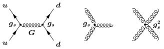
Figure 1: Interactions in QCD.

QCD has the property of asymptotic freedom [6, 7], i.e., the running coupling becomes weak at high energies or short distances. It has been extensively tested in this regime, as is illustrated in Figure 2. At low energies or large distances it becomes strongly coupled (infrared slavery) [8], presumably leading to the confinement of quarks and gluons. QCD incorporates the observed global symmetries of the strong interactions, especially the spontaneously broken global $SU(3)\times SU(3)$ (see, e.g., Gasser:1982ap).

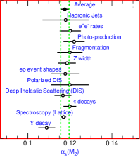
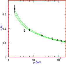
Figure 2: Running of the QCD coupling $\alpha_{s}(\mu)=g_{s}(\mu)^{2}/4\pi$. Left: various experimental determinations extrapolated to $\mu=M_{Z}$ using QCD. Right: experimental values plotted at the $\mu$ at which they are measured. The band is the best fit QCD prediction. Plot courtesy of the Particle Data Group [5], http://pdg.lbl.gov/.

1.2 The Electroweak Theory

The electroweak theory [10, 11, 12] is based on the $SU(2)\times U(1)$ Lagrangian

$$\mathcal{L}_{SU(2)\times U(1)}=\mathcal{L}_{gauge}+\mathcal{L}_{\phi}+\mathcal{L}_{f}+\mathcal{L}_{Yuk}.$$ (5)

The gauge part is

$$\mathcal{L}_{gauge}=-\frac{1}{4}W^{i}_{\mu\nu}W^{\mu\nu i}-\frac{1}{4}B_{\mu\nu}B^{\mu\nu},$$ (6)

where $W^{i}_{\mu},\;i=1,\;2,\;3$ and $B_{\mu}$ are respectively the $SU(2)$ and $U(1)$ gauge fields, with field strength tensors

$$B_{\mu\nu} = \partial_{\mu}B_{\nu}-\partial_{\nu}B_{\mu}$$

$$W^{i}_{\mu\nu} = \partial_{\mu}W_{\nu}^{i}-\partial_{\nu}W_{\mu}^{i}-g\epsilon_{ijk}W^{j}_{\mu}W^{k}_{\nu},$$ (7)

where $g(g^{\prime})$ is the $SU(2)$ $(U(1))$ gauge coupling and $\epsilon_{ijk}$ is the totally antisymmetric symbol. The $SU(2)$ fields have three and four-point self-interactions. $B$ is a $U(1)$ field associated with the weak hypercharge $Y=Q-T^{3}$, where $Q$ and $T^{3}$ are respectively the electric charge operator and the third component of weak $SU(2)$. (Their eigenvalues will be denoted by $y$, $q$, and $t^{3}$, respectively.) It has no self-interactions. The $B$ and $W_{3}$ fields will eventually mix to form the photon and $Z$ boson.

The scalar part of the Lagrangian is

$$\mathcal{L}_{\phi}=(D^{\mu}\phi)^{{\dagger}}D_{\mu}\phi-V(\phi),$$ (8)

where $\phi=\left(\begin{array}[]{c}\phi^{+}\\ \phi^{0}\end{array}\right)$ is a complex Higgs scalar, which is a doublet under $SU(2)$ with $U(1)$ charge $y_{\phi}=+\frac{1}{2}$. The gauge covariant derivative is

$$D_{\mu}\phi=\left(\partial_{\mu}+ig\frac{\tau^{i}}{2}W_{\mu}^{i}+\frac{ig^{\prime}}{2}B_{\mu}\right)\phi,$$ (9)

where the $\tau^{i}$ are the Pauli matrices. The square of the covariant derivative leads to three and four-point interactions between the gauge and scalar fields.

$V(\phi)$ is the Higgs potential. The combination of $SU(2)\times U(1)$ invariance and renormalizability restricts $V$ to the form

$$V(\phi)=+\mu^{2}\phi^{{\dagger}}\phi+\lambda(\phi^{{\dagger}}\phi)^{2}.$$ (10)

For $\mu^{2}<0$ there will be spontaneous symmetry breaking. The $\lambda$ term describes a quartic self-interaction between the scalar fields. Vacuum stability requires $\lambda>0$.

The fermion term is

$$\begin{split}\mathcal{L}_{f}=&\sum^{F}_{m=1}\left(\bar{q}^{0}_{mL}i\not\!\!Dq^{0}_{mL}+\bar{l}^{0}_{mL}i\not\!\!Dl^{0}_{mL}+\bar{u}^{0}_{mR}i\not\!\!Du^{0}_{mR}\right.\\ &\quad+\left.\bar{d}^{0}_{mR}i\not\!\!Dd^{0}_{mR}+\bar{e}^{0}_{mR}i\not\!\!De^{0}_{mR}+\bar{\nu}^{0}_{mR}i\not\!\!D\nu^{0}_{mR}\right).\end{split}$$ (11)

In (11) $m$ is the family index, $F\geq 3$ is the number of families, and $L(R)$ refer to the left (right) chiral projections $\psi_{L(R)}\equiv(1\mp\gamma_{5})\psi/2$. The left-handed quarks and leptons

$$q^{0}_{mL}=\left(\begin{array}[]{c}u^{0}_{m}\\ d^{0}_{m}\end{array}\right)_{L}\ \ \ \ \ l^{0}_{mL}=\left(\begin{array}[]{c}\nu^{0}_{m}\\ e^{-0}_{m}\end{array}\right)_{L}$$ (12)

transform as $SU(2)$ doublets, while the right-handed fields $u^{0}_{mR},\;d^{0}_{mR}$, $e^{-0}_{mR}$, and $\nu^{0}_{mR}$ are singlets. Their $U(1)$ charges are $y_{q_{L}}=\frac{1}{6},\;y_{l_{L}}=-\frac{1}{2},\;y_{\psi_{R}}=q_{\psi}$. The superscript $0$ refers to the weak eigenstates, i.e., fields transforming according to definite $SU(2)$ representations. They may be mixtures of mass eigenstates (flavors). The quark color indices $\alpha=r,\;g,\;b$ have been suppressed. The gauge covariant derivatives are

$$\begin{array}[]{lclclcl}D_{\mu}q^{0}_{mL}&=&\left(\partial_{\mu}+\frac{ig}{2}\vec{\tau}\cdot\vec{W}_{\mu}+\frac{ig^{\prime}}{6}B_{\mu}\right)q^{0}_{mL}&&D_{\mu}u^{0}_{mR}&=&\left(\partial_{\mu}+\frac{2ig^{\prime}}{3}B_{\mu}\right)u^{0}_{mR}\vspace*{2pt}\\ D_{\mu}l^{0}_{mL}&=&\left(\partial_{\mu}+\frac{ig}{2}\vec{\tau}\cdot\vec{W}_{\mu}-\frac{ig^{\prime}}{2}B_{\mu}\right)l^{0}_{mL}&&D_{\mu}d^{0}_{mR}&=&\left(\partial_{\mu}-\frac{ig^{\prime}}{3}B_{\mu}\right)d^{0}_{mR}\vspace*{2pt}\\ &&&&D_{\mu}e^{0}_{mR}&=&\left(\partial_{\mu}-ig^{\prime}B_{\mu}\right)e^{0}_{mR}\vspace*{2pt}\\ &&&&D_{\mu}\nu^{0}_{mR}&=&\partial_{\mu}\nu^{0}_{mR},\end{array}$$ (13)

from which one can read off the gauge interactions between the $W$ and $B$ and the fermion fields. The different transformations of the $L$ and $R$ fields (i.e., the symmetry is chiral) is the origin of parity violation in the electroweak sector. The chiral symmetry also forbids any bare mass terms for the fermions. We have tentatively included $SU(2)$-singlet right-handed neutrinos $\nu^{0}_{mR}$ in (11), because they are required in many models for neutrino mass. However, they are not necessary for the consistency of the theory or for some models of neutrino mass, and it is not certain whether they exist or are part of the low-energy theory.

The standard model is anomaly free for the assumed fermion content. There are no $SU(3)^{3}$ anomalies because the quark assignment is non-chiral, and no $SU(2)^{3}$ anomalies because the representations are real. The $SU(2)^{2}Y$ and $Y^{3}$ anomalies cancel between the quarks and leptons in each family, by what appears to be an accident. The $SU(3)^{2}Y$ and $Y$ anomalies cancel between the $L$ and $R$ fields, ultimately because the hypercharge assignments are made in such a way that $U(1)_{Q}$ will be non-chiral.

The last term in (5) is

$$\begin{split}\mathcal{L}_{Yuk}&=-\sum^{F}_{m,n=1}\left[\Gamma^{u}_{mn}\bar{q}\,^{0}_{mL}\tilde{\phi}u^{0}_{nR}+\Gamma^{d}_{mn}\bar{q}\,^{0}_{mL}\phi d^{0}_{nR}\right.\\ &+\left.\Gamma^{e}_{mn}\bar{l}\,^{0}_{mn}\phi e^{0}_{nR}\ +\Gamma^{\nu}_{mn}\bar{l}\,^{0}_{mL}\tilde{\phi}\nu^{0}_{nR}\right]+h.c.,\end{split}$$ (14)

where the matrices $\Gamma_{mn}$ describe the Yukawa couplings between the single Higgs doublet, $\phi$, and the various flavors $m$ and $n$ of quarks and leptons. One needs representations of Higgs fields with $y=+\frac{1}{2}$ and $-\frac{1}{2}$ to give masses to the down quarks and electrons ($+\frac{1}{2}$), and to the up quarks and neutrinos ($-\frac{1}{2}$). The representation $\phi^{{\dagger}}$ has $y=-\frac{1}{2}$, but transforms as the $2^{*}$ rather than the 2. However, in $SU(2)$ the $2^{*}$ representation is related to the 2 by a similarity transformation, and $\tilde{\phi}\equiv i\tau^{2}\phi^{{\dagger}}=\left(\begin{array}[]{c}\phi^{0^{{\dagger}}}\\ -\phi^{-}\end{array}\right)$ transforms as a 2 with $y_{\tilde{\phi}}=-\frac{1}{2}$. All of the masses can therefore be generated with a single Higgs doublet if one makes use of both $\phi$ and $\tilde{\phi}$. The fact that the fundamental and its conjugate are equivalent does not generalize to higher unitary groups. Furthermore, in supersymmetric extensions of the standard model the supersymmetry forbids the use of a single Higgs doublet in both ways in the Lagrangian, and one must add a second Higgs doublet. Similar statements apply to most theories with an additional $U(1)^{\prime}$ gauge factor, i.e., a heavy $Z^{\prime}$ boson.

2 Spontaneous Symmetry Breaking

Gauge invariance (and therefore renormalizability) does not allow mass terms in the Lagrangian for the gauge bosons or for chiral fermions. Massless gauge bosons are not acceptable for the weak interactions, which are known to be short-ranged. Hence, the gauge invariance must be broken spontaneously [13, 14, 15, 16, 17, 18], which preserves the renormalizability [19, 20, 21, 22]. The idea is that the lowest energy (vacuum) state does not respect the gauge symmetry and induces effective masses for particles propagating through it.

Let us introduce the complex vector

$$v=\langle 0|\phi|0\rangle=\text{ constant},$$ (15)

which has components that are the vacuum expectation values of the various complex scalar fields. $v$ is determined by rewriting the Higgs potential as a function of $v$, $V(\phi)\rightarrow V(v)$, and choosing $v$ such that $V$ is minimized. That is, we interpret $v$ as the lowest energy solution of the classical equation of motion. The quantum theory is obtained by considering fluctuations around this classical minimum, $\phi=v+\phi^{\prime}$.

The single complex Higgs doublet in the standard model can be rewritten in a Hermitian basis as

$$\phi=\left(\begin{array}[]{c}\phi^{+}\\ \phi^{0}\end{array}\right)=\left(\begin{array}[]{c}\frac{1}{\sqrt{2}}(\phi_{1}-i\phi_{2})\\ \frac{1}{\sqrt{2}}(\phi_{3}-i\phi_{4}\end{array}\right),$$ (16)

where $\phi_{i}=\phi_{i}^{{\dagger}}$ represent four Hermitian fields. In this new basis the Higgs potential becomes

$$V(\phi)=\frac{1}{2}\mu^{2}\left(\sum^{4}_{i=1}\phi^{2}_{i}\right)+\frac{1}{4}\lambda\left(\sum^{4}_{i=1}\phi^{2}_{i}\right)^{2},$$ (17)

which is clearly $O(4)$ invariant. Without loss of generality we can choose the axis in this four-dimensional space so that $\langle 0|\phi_{i}|0\rangle=0,\;\ i=1,2,4$ and $\langle 0|\phi_{3}|0\rangle=\nu$. Thus,

$$V(\phi)\rightarrow V(v)=\frac{1}{2}\mu^{2}\nu^{2}+\frac{1}{4}\lambda\nu^{4},$$ (18)

which must be minimized with respect to $\nu$. Two important cases are illustrated in Figure 3. For $\mu^{2}>0$ the minimum occurs at $\nu=0$. That is, the vacuum is empty space and $SU(2)\times U(1)$ is unbroken at the minimum. On the other hand, for $\mu^{2}<0$ the $\nu=0$ symmetric point is unstable, and the minimum occurs at some nonzero value of $\nu$ which breaks the $SU(2)\times U(1)$ symmetry. The point is found by requiring

$$V^{\prime}(\nu)=\nu(\mu^{2}+\lambda\nu^{2})=0,$$ (19)

which has the solution $\nu=\left({-\mu^{2}}/{\lambda}\right)^{1/2}$ at the minimum. (The solution for $-\nu$ can also be transformed into this standard form by an appropriate $O(4)$ transformation.) The dividing point $\mu^{2}=0$ cannot be treated classically. It is necessary to consider the one loop corrections to the potential, in which case it is found that the symmetry is again spontaneously broken [25].

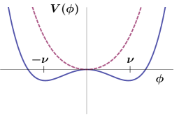
Figure 3: The Higgs potential $V(\phi)$ for $\mu^{2}>0$ (dashed line) and $\mu^{2}<0$ (solid line).

We are interested in the case $\mu^{2}<0$, for which the Higgs doublet is replaced, in first approximation, by its classical value $\phi\rightarrow\frac{1}{\sqrt{2}}\left(\begin{array}[]{c}0\\ \nu\end{array}\right)\equiv v$. The generators $L^{1}$, $L^{2}$, and $L^{3}-Y$ are spontaneously broken (e.g., $L^{1}v\neq 0$). On the other hand, the vacuum carries no electric charge ($Qv=(L^{3}+Y)v=0$), so the $U(1)_{Q}$ of electromagnetism is not broken. Thus, the electroweak $SU(2)\times U(1)$ group is spontaneously broken to the $U(1)_{Q}$ subgroup, $SU(2)\times U(1)_{Y}\rightarrow U(1)_{Q}$.

To quantize around the classical vacuum, write $\phi=v+\phi^{\prime}$, where $\phi^{\prime}$ are quantum fields with zero vacuum expectation value. To display the physical particle content it is useful to rewrite the four Hermitian components of $\phi^{\prime}$ in terms of a new set of variables using the Kibble transformation [26]:

$$\phi=\frac{1}{\sqrt{2}}e^{i\sum\xi^{i}L^{i}}\left(\begin{array}[]{c}0\\ \nu+H\end{array}\right).$$ (20)

$H$ is a Hermitian field which will turn out to be the physical Higgs scalar. If we had been dealing with a spontaneously broken global symmetry the three Hermitian fields $\xi^{i}$ would be the massless pseudoscalar Nambu-Goldstone bosons [27, 28, 29, 30] that are necessarily associated with broken symmetry generators. However, in a gauge theory they disappear from the physical spectrum. To see this it is useful to go to the unitary gauge

$$\phi\rightarrow\phi^{\prime}=e^{-i\sum\xi^{i}L^{i}}\phi=\frac{1}{\sqrt{2}}\left(\begin{array}[]{c}0\\ \nu+H\end{array}\right),$$ (21)

in which the Goldstone bosons disappear. In this gauge, the scalar covariant kinetic energy term takes the simple form

$$(D_{\mu}\phi)^{{\dagger}}D^{\mu}\phi = \frac{1}{2}(0\;\nu)\left[\frac{g}{2}\tau^{i}W^{i}_{\mu}+\frac{g^{\prime}}{2}B_{\mu}\right]^{2}\left(\begin{array}[]{c}0\\ \nu\end{array}\right)+H\text{ terms}$$ (24)

$$\rightarrow M^{2}_{W}W^{+\mu}W^{-}_{\mu}+\frac{M_{Z}^{2}}{2}Z^{\mu}Z_{\mu}+H\text{ terms},$$ (25)

where the kinetic energy and gauge interaction terms of the physical $H$ particle have been omitted. Thus, spontaneous symmetry breaking generates mass terms for the $W$ and $Z$ gauge bosons

$$W^{\pm} = \frac{1}{\sqrt{2}}(W^{1}\mp iW^{2})$$

$$Z = -\sin\theta_{W}B+\cos\theta_{W}W^{3}.$$ (26)

The photon field

$$A=\cos\theta_{W}B+\sin\theta_{W}W^{3}$$ (27)

remains massless. The masses are

$$M_{W}=\frac{g\nu}{2}$$ (28)

and

$$M_{Z}=\sqrt{g^{2}+g^{\prime 2}}\frac{\nu}{2}=\frac{M_{W}}{\cos\theta_{W}},$$ (29)

where the weak angle is defined by

$$\tan\theta_{W}\equiv\frac{g^{\prime}}{g}\ \Rightarrow\ \sin^{2}\theta_{W}=1-\frac{M_{W}^{2}}{M_{Z}^{2}}.$$ (30)

One can think of the generation of masses as due to the fact that the $W$ and $Z$ interact constantly with the condensate of scalar fields and therefore acquire masses, in analogy with a photon propagating through a plasma. The Goldstone boson has disappeared from the theory but has reemerged as the longitudinal degree of freedom of a massive vector particle.

It will be seen below that $G_{F}/\sqrt{2}\sim g^{2}/8M^{2}_{W}$, where $G_{F}=1.16637(5)\times 10^{-5}$ GeV^-2 is the Fermi constant determined by the muon lifetime. The weak scale $\nu$ is therefore

$$\nu=2M_{W}/g\simeq(\sqrt{2}G_{F})^{-1/2}\simeq 246\text{ GeV}.$$ (31)

Similarly, $g=e/\sin\theta_{W}$, where $e$ is the electric charge of the positron. Hence, to lowest order

$$M_{W}=M_{Z}\cos\theta_{W}\sim\frac{(\pi\alpha/\sqrt{2}G_{F})^{1/2}}{\sin\theta_{W}},$$ (32)

where $\alpha\sim 1/137.036$ is the fine structure constant. Using $\sin^{2}\theta_{W}\sim 0.23$ from neutral current scattering, one expects $M_{W}\sim 78$ GeV, and $M_{Z}\sim 89$ GeV. (These predictions are increased by $\sim(2-3)$ GeV by loop corrections.) The $W$ and $Z$ were discovered at CERN by the UA1 [31] and UA2 [32] groups in 1983. Subsequent measurements of their masses and other properties have been in excellent agreement with the standard model expectations (including the higher-order corrections) [5]. The current values are

$$M_{W}=80.398\pm 0.025\text{ GeV},\qquad M_{Z}=91.1876\pm 0.0021\text{ GeV}.$$ (33)

3 The Higgs and Yukawa Interactions

The full Higgs part of $\mathcal{L}$ is

$$\begin{split}\mathcal{L}_{\phi}&=(D^{\mu}\phi)^{{\dagger}}D_{\mu}\phi-V(\phi)\\ &=M_{W}^{2}W^{\mu+}W_{\mu}^{-}\left(1+\frac{H}{\nu}\right)^{2}+\frac{1}{2}M_{Z}^{2}Z^{\mu}Z_{\mu}\left(1+\frac{H}{\nu}\right)^{2}\\ &+\frac{1}{2}\left(\partial_{\mu}H\right)^{2}-V(\phi).\end{split}$$ (34)

The second line includes the $W$ and $Z$ mass terms and also the $ZZH^{2}$, $W^{+}W^{-}H^{2}$ and the induced $ZZH$ and $W^{+}W^{-}H$ interactions, as shown in Table 3 and Figure 4. The last line includes the canonical Higgs kinetic energy term and the potential.

Feynman rules for the gauge and Higgs interactions after SSB, taking combinatoric factors into account. The momenta and quantum numbers flow into the vertex. Note the dependence on $M/\nu$ or $M^{2}/\nu$. $W^{+}_{\mu}W_{\nu}^{-}H$: $\frac{1}{2}ig_{\mu\nu}g^{2}\nu=2ig_{\mu\nu}\frac{M_{W}^{2}}{\nu}$ $W^{+}_{\mu}W_{\nu}^{-}H^{2}$: $\frac{1}{2}ig_{\mu\nu}g^{2}=2ig_{\mu\nu}\frac{M_{W}^{2}}{\nu^{2}}$ $Z_{\mu}Z_{\nu}H$: $\frac{ig_{\mu\nu}g^{2}\nu}{2\cos^{2}\theta_{W}}=2ig_{\mu\nu}\frac{M_{Z}^{2}}{\nu}$ $Z_{\mu}Z_{\nu}H^{2}$: $\frac{ig_{\mu\nu}g^{2}}{2\cos^{2}\theta_{W}}=2ig_{\mu\nu}\frac{M_{Z}^{2}}{\nu^{2}}$ $H^{3}$: $-6i\lambda\nu=-3i\frac{M_{H}^{2}}{\nu}$ $H^{4}$: $-6i\lambda=-3i\frac{M_{H}^{2}}{\nu^{2}}$ $H\bar{f}f$: $-ih_{f}=-i\frac{m_{f}}{\nu}$ $W^{+}_{\mu}(p)\gamma_{\nu}(q)W^{-}_{\sigma}(r)\qquad ie\,{\cal C}_{\mu\nu\sigma}(p,q,r)$ $W^{+}_{\mu}(p)Z_{\nu}(q)W^{-}_{\sigma}(r)\qquad i\frac{e}{\tan\theta_{W}}{\cal C}_{\mu\nu\sigma}(p,q,r)$ $W^{+}_{\mu}W^{+}_{\nu}W^{-}_{\sigma}W^{-}_{\rho}\qquad i\frac{e^{2}}{\sin^{2}\theta_{W}}{\cal Q}_{\mu\nu\rho\sigma}$ $W^{+}_{\mu}Z_{\nu}\gamma_{\sigma}W^{-}_{\rho}\qquad-i\frac{e^{2}}{\tan\theta_{W}}{\cal Q}_{\mu\rho\nu\sigma}$ $W^{+}_{\mu}Z_{\nu}Z_{\sigma}W^{-}_{\rho}\qquad-i\frac{e^{2}}{\tan^{2}\theta_{W}}{\cal Q}_{\mu\rho\nu\sigma}$ $W^{+}_{\mu}\gamma_{\nu}\gamma_{\sigma}W^{-}_{\rho}\qquad-ie^{2}{\cal Q}_{\mu\rho\nu\sigma}$ ${\cal C}_{\mu\nu\sigma}(p,q,r)\equiv g_{\mu\nu}(q-p)_{\sigma}+g_{\mu\sigma}(p-r)_{\nu}+g_{\nu\sigma}(r-q)_{\mu}$ ${\cal Q}_{\mu\nu\rho\sigma}\equiv 2g_{\mu\nu}g_{\rho\sigma}-g_{\mu\rho}g_{\nu\sigma}-g_{\mu\sigma}g_{\nu\rho}$

Figure 4: Higgs interaction vertices in the standard model.

After symmetry breaking the Higgs potential in unitary gauge becomes

$$V(\phi)=-\frac{\mu^{4}}{4\lambda}-\mu^{2}H^{2}+\lambda\nu H^{3}+\frac{\lambda}{4}H^{4}.$$ (35)

The first term in the Higgs potential $V$ is a constant, $\langle 0|V(\nu)|0\rangle=-\mu^{4}/4\lambda$. It reflects the fact that $V$ was defined so that $V(0)=0$, and therefore $V<0$ at the minimum. Such a constant term is irrelevant to physics in the absence of gravity, but will be seen in Section 5 to be one of the most serious problems of the SM when gravity is incorporated because it acts like a cosmological constant much larger (and of opposite sign) than is allowed by observations. The third and fourth terms in $V$ represent the induced cubic and quartic interactions of the Higgs scalar, shown in Table 3 and Figure 4.

The second term in $V$ represents a (tree-level) mass

$$M_{H}=\sqrt{-2\mu^{2}}=\sqrt{2\lambda}\nu,$$ (36)

for the Higgs boson. The weak scale is given in (31), but the quartic Higgs coupling $\lambda$ is unknown, so $M_{H}$ is not predicted. A priori, $\lambda$ could be anywhere in the range $0\leq\lambda<\infty$. There is an experimental lower limit $M_{H}\gtrsim 114.4$ GeV at 95% cl from LEP [33]. Otherwise, the decay $Z\rightarrow Z^{*}H$ would have been observed.

There are also plausible theoretical limits. If $\lambda>\mathcal{O}(1)$ the theory becomes strongly coupled $(M_{H}>\mathcal{O}(1$ TeV)). There is not really anything wrong with strong coupling a priori. However, there are fairly convincing triviality limits, which basically say that the running quartic coupling would become infinite within the domain of validity of the theory if $\lambda$ and therefore $M_{H}$ is too large. If one requires the theory to make sense to infinite energy, one runs into problems for any $\lambda$. However, one only needs for the theory to hold up to the next mass scale $\Lambda$, at which point the standard model breaks down. In that case [34, 35, 36],

$$M_{H}<\left\{\begin{array}[]{l}\mathcal{O}(180)\;GeV,\;\Lambda\sim M_{P}\\ O(700)\;GeV,\;\Lambda\sim 2M_{H}.\end{array}\right.$$ (37)

The more stringent limit of $O(180)$ GeV obtains for $\Lambda$ of order of the Planck scale $M_{P}=G_{N}^{-1/2}\sim 10^{19}$ GeV. If one makes the less restrictive assumption that the scale $\Lambda$ of new physics can be small, one obtains a weaker limit. Nevertheless, for the concept of an elementary Higgs field to make sense one should require that the theory be valid up to something of order of $2M_{H}$, which implies that $M_{H}<O$(700) GeV. These estimates rely on perturbation theory, which breaks down for large $\lambda$. However, they can be justified by nonperturbative lattice calculations [37, 38, 39], which suggest an absolute upper limit of $650-700$ GeV. There are also comparable upper bounds from the validity of unitarity at the tree level [40], and lower limits from vacuum stability [34, 41, 42, 43]. The latter again depends on the scale $\Lambda$, and requires $M_{H}\gtrsim$ 130 GeV for $\Lambda=M_{P}$ (lowered to $\sim 115$ GeV if one allows a sufficiently long-lived metastable vacuum [42, 43]), with a weaker constraint for lower $\Lambda$.

The Yukawa interaction in the unitary gauge becomes

$$-\mathcal{L}_{Yuk} \rightarrow \sum^{F}_{m,n=1}\bar{u}^{0}_{mL}\Gamma^{u}_{mn}\left(\frac{\nu+H}{\sqrt{2}}\right)u^{0}_{mR}+(d,e,\nu)\text{ terms}\;+\;\;h.c.$$ (38)

$$= \bar{u}^{0}_{L}\left(M^{u}+h^{u}H\right)u^{0}_{R}+(d,e,\nu)\text{ terms}\;+h.c.,$$

where in the second form $u^{0}_{L}=\left(u^{0}_{1L}u^{0}_{2L}\cdots u^{0}_{FL}\right)^{T}$ is an $F$-component column vector, with a similar definition for $u_{R}^{0}$. $M^{u}$ is an $F\times F$ fermion mass matrix $M^{u}_{mn}=\Gamma^{u}_{mn}{\nu}/{\sqrt{2}}$ induced by spontaneous symmetry breaking, and $h^{u}=M^{u}/\nu={gM^{u}}/{2M_{W}}$ is the Yukawa coupling matrix.

In general $M$ is not diagonal, Hermitian, or symmetric. To identify the physical particle content it is necessary to diagonalize $M$ by separate unitary transformations $A_{L}$ and $A_{R}$ on the left- and right-handed fermion fields. (In the special case that $M^{u}$ is Hermitian one can take $A_{L}=A_{R}$). Then,

$$A_{L}^{u{\dagger}}M^{u}A^{u}_{R}=M^{u}_{D}=\left(\begin{array}[]{ccc}m_{u}&0&0\\ 0&m_{c}&0\\ 0&0&m_{t}\end{array}\right)$$ (39)

is a diagonal matrix with eigenvalues equal to the physical masses of the charge $\frac{2}{3}$ quarks. Similarly, one diagonalizes the down quark, charged lepton, and neutrino mass matrices by

$$\begin{split}A^{d{\dagger}}_{L}M^{d}A^{d}_{R}&=M^{d}_{D}\\ A^{e{\dagger}}_{L}M^{e}A^{e}_{R}&=M^{e}_{D}\\ A^{\nu{\dagger}}_{L}M^{\nu}A^{\nu}_{R}&=M^{\nu}_{D}.\end{split}$$ (40)

In terms of these unitary matrices we can define mass eigenstate fields $u_{L}=A_{L}^{u{\dagger}}u_{L}^{0}=(u_{L}\ c_{L}\ t_{L})^{T}$, with analogous definitions for $u_{R}=A_{R}^{u{\dagger}}u_{R}^{0}$, $d_{L,R}=A_{L,R}^{d{\dagger}}d_{L,R}^{0}$, $e_{L,R}=A_{L,R}^{e{\dagger}}e_{L,R}^{0}$, and $\nu_{L,R}=A_{L,R}^{\nu{\dagger}}\nu_{L,R}^{0}$. Typical estimates of the quark masses are [9, 5] $m_{u}\sim 1.5-3$ MeV, $m_{d}\sim 3-7$ MeV, $m_{s}\sim 70-120$ MeV, $m_{c}\sim 1.5-1.8$ GeV, $m_{b}\sim 4.7-5.0$ GeV, and $m_{t}=170.9\pm 1.8$ GeV. These are the current masses: for QCD their effects are identical to bare masses in the QCD Lagrangian. They should not be confused with the constituent masses of order 300 MeV generated by the spontaneous breaking of chiral symmetry in the strong interactions. Including QCD renormalizations, the $u,\;d$, and $s$ masses are running masses evaluated at 2 GeV², while $m_{c,b,t}$ are pole masses.

So far we have only allowed for ordinary Dirac mass terms of the form $\bar{\nu}^{0}_{mL}\nu^{0}_{nR}$ for the neutrinos, which can be generated by the ordinary Higgs mechanism. Another possibility are lepton number violating Majorana masses, which require an extended Higgs sector or higher-dimensional operators. It is not clear yet whether Nature utilizes Dirac masses, Majorana masses, or both. What is known, is that the neutrino mass eigenvalues are tiny compared to the other masses, $\lesssim{\cal O}(0.1)$ eV, and most experiments are insensitive to them. In describing such processes, one can ignore $\Gamma^{\nu}$, and the $\nu_{R}$ effectively decouple. Since $M^{\nu}\sim 0$ the three mass eigenstates are effectively degenerate with eigenvalues $0$, and the eigenstates are arbitrary. That is, there is nothing to distinguish them except their weak interactions, so we can simply define $\nu_{e},\;\nu_{\mu},\;\nu_{\tau}$ as the weak interaction partners of the $e,\;\mu$, and $\tau$, which is equivalent to choosing $A_{L}^{\nu}\equiv A_{L}^{e}$ so that $\nu_{L}=A_{L}^{e{\dagger}}\nu_{L}^{0}$. Of course, this is not appropriate for physical processes, such as oscillation experiments, that are sensitive to the masses or mass differences.

In terms of the mass eigenstate fermions,

$$-\mathcal{L}_{Yuk}=\sum_{i}m_{i}\bar{\psi}_{i}\psi_{i}\left(1+\frac{g}{2M_{W}}H\right)=\sum_{i}m_{i}\bar{\psi}_{i}\psi_{i}\left(1+\frac{H}{\nu}\right).$$ (41)

The coupling of the physical Higgs boson to the $i^{th}$ fermion is $gm_{i}/2M_{W}$, which is very small except for the top quark. The coupling is flavor-diagonal in the minimal model: there is just one Yukawa matrix for each type of fermion, so the mass and Yukawa matrices are diagonalized by the same transformations. In generalizations in which more than one Higgs doublet couples to each type of fermion there will in general be flavor-changing Yukawa interactions involving the physical neutral Higgs fields [48]. There are stringent limits on such couplings; for example, the $K_{L}-K_{S}$ mass difference implies $h/M_{H}<10^{-6}\,\text{GeV}^{-1}$, where $h$ is the $\bar{d}s$ Yukawa coupling [49, 50, 51].

4 The Gauge Interactions

The major quantitative tests of the electroweak standard model involve the gauge interactions of fermions and the properties of the gauge bosons. The charged current weak interactions of the Fermi theory and its extension to the intermediate vector boson theory are incorporated into the standard model, as is quantum electrodynamics. The theory successfully predicted the existence and properties of the weak neutral current. In this section I summarize the structure of the gauge interactions of fermions.

4.1 The Charged Current

The interaction of the $W$ bosons to fermions is given by

$$\mathcal{L}=-\frac{g}{2\sqrt{2}}\left(J^{\mu}_{W}W^{-}_{\mu}+J^{\mu{\dagger}}_{W}W^{+}_{\mu}\right),$$ (42)

where the weak charge-raising current is

$$\begin{split}J_{W}^{\mu{\dagger}}&=\sum^{F}_{m=1}\left[\bar{\nu}_{m}^{0}\gamma^{\mu}(1-\gamma^{5})e^{0}_{m}+\bar{u}_{m}^{0}\gamma^{\mu}(1-\gamma^{5})d^{0}_{m}\right]\\ &=(\bar{\nu}_{e}\bar{\nu}_{\mu}\bar{\nu}_{\tau})\gamma^{\mu}(1-\gamma^{5})V_{\ell}\left(\begin{array}[]{c}e^{-}\\ \mu^{-}\\ \tau^{-}\end{array}\right)+(\bar{u}\;\bar{c}\;\bar{t})\gamma^{\mu}(1-\gamma^{5})V_{q}\left(\begin{array}[]{c}d\\ s\\ b\end{array}\right).\end{split}$$ (43)

$J^{\mu{\dagger}}_{W}$ has a $V-A$ form, i.e., it violates parity and charge conjugation maximally. The fermion gauge vertices are shown in Figure 5.

Figure 5: The fermion gauge interaction vertices in the standard electroweak model. $g_{V}^{f}\equiv t^{3}_{fL}-2\sin^{2}\theta_{W}q_{f}$ and $g_{A}^{f}\equiv t^{3}_{fL}$, where $t^{3}_{uL}=t^{3}_{\nu L}=+\frac{1}{2}$, while $t^{3}_{dL}=t^{3}_{eL}=-\frac{1}{2}$. The $\bar{d}_{j}u_{i}W^{-}$ vertex is the same as for $\bar{u}_{i}d_{j}W^{+}$ except $V_{qij}\rightarrow\left(V^{\dagger}_{q}\right)_{ji}=V^{\ast}_{qij}$. The lepton-$W^{\pm}$ vertices are obtained from the quark ones by $u_{i}\rightarrow\nu_{i}$, $d_{j}\rightarrow e^{-}_{j}$, and $V_{q}\rightarrow V_{\ell}$.

The mismatch between the unitary transformations relating the weak and mass eigenstates for the up and down-type quarks leads to the presence of the $F\times F$ unitary matrix $V_{q}\equiv A^{u{\dagger}}_{L}A^{d}_{L}$ in the current. This is the Cabibbo-Kobayashi-Maskawa (CKM) matrix [52, 53], which is ultimately due to the mismatch between the weak and Yukawa interactions. For $F=2$ families $V_{q}$ takes the familiar form

$$V_{Cabibbo}=\left(\begin{array}[]{cc}\cos\theta_{c}&\sin\theta_{c}\\ -\sin\theta_{c}&\cos\theta_{c}\end{array}\right),$$ (44)

where $\sin\theta_{c}\simeq 0.22$ is the Cabibbo angle. This form gives a good zero^th-order approximation to the weak interactions of the $u,d,s$ and $c$ quarks; their coupling to the third family, though non-zero, is very small. Including these couplings, the 3-family CKM matrix is

$$V_{CKM}=\left(\begin{array}[]{ccc}V_{ud}&V_{us}&V_{ub}\\ V_{cd}&V_{cs}&V_{cb}\\ V_{td}&V_{ts}&V_{tb}\end{array}\right)\sim\left(\begin{array}[]{ccc}1&\lambda&\lambda^{3}\\ \lambda&1&\lambda^{2}\\ \lambda^{3}&\lambda^{2}&1\end{array}\right),$$ (45)

where the $V_{ij}$ may involve a $CP$-violating phase. The second form, with $\lambda=\sin\theta_{c}$, is an easy to remember approximation to the observed magnitude of each element [54], which displays a suggestive but not well understood hierarchical structure. These are order of magnitude only; each element may be multiplied by a phase and a coefficient of ${\cal O}(1)$.

$V_{\ell}\equiv A^{\nu\dagger}_{L}A^{e}_{L}$ in (43) is the analogous leptonic mixing matrix. It is critical for describing neutrino oscillations and other processes sensitive to neutrino masses. However, for processes for which the neutrino masses are negligible we can effectively set $V_{\ell}=I$ (more precisely, $V_{\ell}$ will only enter such processes in the combination $V_{\ell}^{\dagger}V_{\ell}=I$, so it can be ignored).

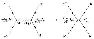
Figure 6: A weak interaction mediated by the exchange of a $W$ and the effective four-fermi interaction that it generates if the four-momentum transfer $Q$ is sufficiently small.

The interaction between fermions mediated by the exchange of a $W$ is illustrated in Figure 6. In the limit $|Q^{2}|\ll M_{W}^{2}$ the momentum term in the $W$ propagator can be neglected, leading to an effective zero-range (four-fermi) interaction

$$-\mathcal{L}^{cc}_{eff}=\frac{G_{F}}{\sqrt{2}}J^{\mu}_{W}J^{{\dagger}}_{W\mu},$$ (46)

where the Fermi constant is identified as

$$\frac{G_{F}}{\sqrt{2}}\simeq\frac{g^{2}}{8M_{W}^{2}}=\frac{1}{2\nu^{2}}.$$ (47)

Thus, the Fermi theory is an approximation to the standard model valid in the limit of small momentum transfer. From the muon lifetime, $G_{F}=1.16637(5)\times 10^{-5}$ GeV^-2, which implies that the weak interaction scale defined by the VEV of the Higgs field is $\nu=\sqrt{2}\langle 0|\phi^{0}|0\rangle\simeq 246$ GeV.

The charged current weak interaction as described by (46) has been successfully tested in a large variety of weak decays [55, 56, 57, 5], including $\beta$, $K$, hyperon, heavy quark, $\mu$, and $\tau$ decays. In particular, high precision measurements of $\beta$, $\mu$, and $\tau$ decays are a sensitive probe of extended gauge groups involving right-handed currents and other types of new physics, as is described in the chapters by Deutsch and Quin; Fetscher and Gerber; and Herczeg in Langacker:268088. Tests of the unitarity of the CKM matrix are important in searching for the presence of fourth family or exotic fermions and for new interactions [58]. The standard theory has also been successfully probed in neutrino scattering processes such as $\nu_{\mu}e\rightarrow\mu^{-}\nu_{e},\nu_{\mu}n\rightarrow\mu^{-}p,\nu_{\mu}N\rightarrow\mu^{-}X$. It works so well that the charged current neutrino-hadron interactions are used more as a probe of the structure of the hadrons and QCD than as a test of the weak interactions.

Weak charged current effects have also been observed in higher orders, such as in $K^{0}-\bar{K}^{0}$, $D^{0}-\bar{D}^{0}$, and $B^{0}-\bar{B}^{0}$ mixing, and in $CP$ violation in $K$ and $B$ decays [5]. For these higher order processes the full theory must be used because large momenta occur within the loop integrals. An example of the consistency between theory and experiment is shown in Figure 7.

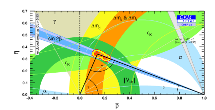
Figure 7: The unitarity triangle, showing the consistency of various $CP$-conserving and $CP$-violating observables from the $K$ and $B$ systems. $\bar{\rho}$ and $\bar{\eta}$ are the same as $\rho$ and $\eta$ up to higher order corrections, where $\rho-i\eta=V_{ub}/(V_{cb}V_{us})$. Plot courtesy of the CKMfitter group [59], http://ckmfitter.in2p3.fr.

4.2 QED

The standard model incorporates all of the (spectacular) successes of quantum electrodynamics (QED), which is based on the $U(1)_{Q}$ subgroup that remains unbroken after spontaneous symmetry breaking. The relevant part of the Lagrangian density is

$$\mathcal{L}=-\frac{gg^{\prime}}{\sqrt{g^{2}+g^{\prime 2}}}J^{\mu}_{Q}(\cos\theta_{W}B_{\mu}+\sin\theta_{W}W^{3}_{\mu}),$$ (48)

where the linear combination of neutral gauge fields is just the photon field $A_{\mu}$. This reproduces the QED interaction provided one identifies the combination of couplings

$$e=g\sin\theta_{W}$$ (49)

as the electric charge of the positron, where $\tan\theta_{W}\equiv g^{\prime}/g$. The electromagnetic current is given by

$$\begin{split}J^{\mu}_{Q}&=\sum^{F}_{m=1}\left[\frac{2}{3}\bar{u}^{0}_{m}\gamma^{\mu}u^{0}_{m}-\frac{1}{3}\bar{d}^{0}_{m}\gamma^{\mu}d_{m}^{0}-\bar{e}^{0}_{m}\gamma^{\mu}e^{0}_{m}\right]\\ &=\sum^{F}_{m=1}\left[\frac{2}{3}\bar{u}_{m}\gamma^{\mu}u_{m}-\frac{1}{3}\bar{d}_{m}\gamma^{\mu}d_{m}-\bar{e}_{m}\gamma^{\mu}e_{m}\right].\end{split}$$ (50)

It takes the same form when written in terms of either weak or mass eigenstates because all fermions which mix with each other have the same electric charge. Thus, the electromagnetic current is automatically flavor-diagonal.

Quantum electrodynamics is the most successful theory in physics when judged in terms of the theoretical and experimental precision of its tests. A detailed review is given in Kinoshita:213617. The classical atomic tests of QED, such as the Lamb shift, atomic hyperfine splittings, muonium ($\mu^{+}e^{-}$ bound states), and positronium ($e^{+}e^{-}$ bound states) are reviewed in Karshenboim:2005iy. The most precise determinations of $\alpha$ and the other physical constants are surveyed in Mohr:2008fa. High energy tests are described in Wu:1984ik,Kiesling:113108. The currently most precise measurements of $\alpha$ are compared in Table 4.2. The approximate agreement of these determinations, which involves the calculation of the electron anomalous magnetic moment $a_{e}=(g_{e}-2)/2$ to high order, validates not only QED but the entire formalism of gauge invariance and renormalization theory. Other basic predictions of gauge invariance (assuming it is not spontaneously broken, which would lead to electric charge nonconservation), are that the photon mass $m_{\gamma}$ and its charge $q_{\gamma}$ (in units of $e$) should vanish. The current upper bounds are extremely impressive [5]

$$m_{\gamma}<1\times 10^{-18}\text{ eV },\qquad q_{\gamma}<5\times 10^{-30},$$ (51)

based on astrophysical effects (the survival of the Solar magnetic field and limits on the dispersion of light from pulsars).

There is a possibly significant discrepancy between the high precision measurement of the anomalous magnetic moment of the muon $a_{\mu}^{exp}=11~{}659~{}208.0(5.4)(3.3)\times 10^{-10}$ by the Brookhaven 821 experiment [65], and the theoretical expectation, for which the purely QED part has been calculated to 4 loops and the leading 5 loop contributions estimated (see the review by Höcker and Marciano in Amsler:2008zz). In addition to the QED part, there are weak interaction corrections (2 loop) and hadronic vacuum polarization and hadronic light by light scattering corrections. There is some theoretical uncertainty in the hadronic corrections. Using estimates of the hadronic vacuum polarization using the measured cross section for $e^{+}e^{-}\rightarrow$ hadrons in a dispersion relation, one finds

$$a_{\mu}^{SM}=116~{}591~{}788(58)\times 10^{-11}\ \Rightarrow\ \Delta a_{\mu}=a_{\mu}^{exp}-a_{\mu}^{SM}=292(86)\times 10^{-11},$$ (52)

a 3.4$\sigma$ discrepancy. However, using hadronic $\tau$ decay instead, the discrepancy is reduced to only $0.9\sigma$. If real, the discrepancy could single the effects of new physics, such as the contributions of relatively light supersymmetric particles. For example, the central value of the discrepancy in (52) would be accounted for [66] if

$$m_{SUSY}\sim 67\sqrt{\tan\beta}\text{ GeV},$$ (53)

where $m_{SUSY}$ is the typical mass of the relevant sleptons, neutralinos, and charginos, and $\tan\beta$ is the ratio of the expectation values of the two Higgs doublets in the theory.

Most precise determinations of the fine structure constant $\alpha=e^{2}/4\pi$. $\Delta_{e}$ is defined as $\left[\alpha^{-1}-\alpha^{-1}(a_{e})\right]\times 10^{6}$. Detailed descriptions and references are given in Mohr:2008fa. Experiment Value of $\alpha^{-1}$ Precision $\Delta_{e}$ $a_{e}=(g_{e}-2)/2$ $137.035~{}999~{}683~{}(94)$ $[6.9\times 10^{-10}]$         – $h/m$ (Rb, Cs) $137.035~{}999~{}35~{}(69)$ $[5.0\times 10^{-9}]$ $0.33\pm 0.69$ Quantum Hall $137.036~{}003~{}0~{}(25)$ $[1.8\times 10^{-8}]$ $-3.3\pm 2.5$ $h/m$ (neutron) $137.036~{}007~{}7~{}(28)$ $[2.1\times 10^{-8}]$ $-8.0\pm 2.8$ $\gamma_{p,^{3}He}$ (J. J.) $137.035~{}987~{}5~{}(43)$ $[3.1\times 10^{-8}]$ $12.2\pm 4.3$ $\mu^{+}e^{-}$ hyperfine $137.036~{}001~{}7~{}(80)$ $[5.8\times 10^{-8}]$ $-2.0\pm 8.0$

4.3 The Neutral Current

The third class of gauge interactions is the weak neutral current, which was predicted by the $SU(2)\times U(1)$ model. The relevant interaction is

$$\mathcal{L}=-\frac{\sqrt{g^{2}+g^{\prime 2}}}{2}J^{\mu}_{Z}\left(-\sin\theta_{W}B_{\mu}+\cos\theta_{W}W^{3}_{\mu}\right)=-\frac{g}{2\cos\theta_{W}}J^{\mu}_{Z}Z_{\mu},$$ (54)

where the combination of neutral fields is the massive $Z$ boson field. The strength is conveniently rewritten as $g/(2\cos\theta_{W})$, which follows from $\cos\theta_{W}=g/\sqrt{g^{2}+g^{\prime 2}}$.

The weak neutral current is given by

$$\begin{split}J^{\mu}_{Z}&=\sum_{m}\left[\bar{u}^{0}_{mL}\gamma^{\mu}u^{0}_{mL}-\bar{d}^{0}_{mL}\gamma^{\mu}d^{0}_{mL}+\bar{\nu}^{0}_{mL}\gamma^{\mu}\nu^{0}_{mL}-\bar{e}^{0}_{mL}\gamma^{\mu}e^{0}_{mL}\right]\\ &\qquad\qquad-2\sin^{2}\theta_{W}J^{\mu}_{Q}\\ &=\sum_{m}\left[\bar{u}_{mL}\gamma^{\mu}u_{mL}-\bar{d}_{mL}\gamma^{\mu}d_{mL}+\bar{\nu}_{mL}\gamma^{\mu}\nu_{mL}-\bar{e}_{mL}\gamma^{\mu}e_{mL}\right]\\ &\qquad\qquad-2\sin^{2}\theta_{W}J^{\mu}_{Q}.\end{split}$$ (55)

Like the electromagnetic current $J^{\mu}_{Z}$ is flavor-diagonal in the standard model; all fermions which have the same electric charge and chirality and therefore can mix with each other have the same $SU(2)\times U(1)$ assignments, so the form is not affected by the unitary transformations that relate the mass and weak bases. It was for this reason that the GIM mechanism [67] was introduced into the model, along with its prediction of the charm quark. Without it the $d$ and $s$ quarks would not have had the same $SU(2)\times U(1)$ assignments, and flavor-changing neutral currents would have resulted. The absence of such effects is a major restriction on many extensions of the standard model involving exotic fermions [68]. The neutral current has two contributions. The first only involves the left-chiral fields and is purely $V-A$. The second is proportional to the electromagnetic current with coefficient $\sin^{2}\theta_{W}$ and is purely vector. Parity is therefore violated in the neutral current interaction, though not maximally.

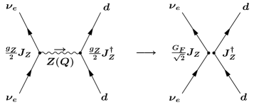
Figure 8: Typical neutral current interaction mediated by the exchange of the $Z$, which reduces to an effective four-fermi interaction in the limit that the momentum transfer $Q$ can be neglected. $g_{Z}$ is defined as $\sqrt{g^{2}+g^{\prime 2}}$.

In an interaction between fermions in the limit that the momentum transfer is small compared to $M_{Z}$ one can neglect the $Q^{2}$ term in the propagator, and the interaction reduces to an effective four-fermi interaction

$$-\mathcal{L}^{NC}_{eff}=\frac{G_{F}}{\sqrt{2}}J^{\mu}_{Z}J_{Z\mu}.$$ (56)

The coefficient is the same as in the charged case because

$$\frac{G_{F}}{\sqrt{2}}=\frac{g^{2}}{8M_{W}^{2}}=\frac{g^{2}+g^{\prime 2}}{8M_{Z}^{2}}.$$ (57)

That is, the difference in $Z$ couplings compensates the difference in masses in the propagator.

The weak neutral current was discovered at CERN in 1973 by the Gargamelle bubble chamber collaboration [69] and by HPW at Fermilab [70] shortly thereafter, and since that time $Z$ exchange and $\gamma-Z$ interference processes have been extensively studied in many interactions, including $\nu e\rightarrow\nu e,\;\nu N\rightarrow\nu N,\;\nu N\rightarrow\nu X$; polarized $e^{-}$-hadron and $\mu$-hadron scattering; atomic parity violation; and in $e^{+}e^{-}$ and $Z$-pole reactions. Along with the properties of the $W$ and $Z$ they have been the primary quantitative test of the unification part of the standard electroweak model.

The results of these experiments have generally been in excellent agreement with the predictions of the SM, indicating that the basic structure is correct to first approximation and constraining the effects of possible new physics. One exception are the recent precise measurements of the ratios of neutral to charged current deep inelastic neutrino scattering by the NuTeV collaboration at Fermilab [77], with a sign-selected beam which allowed them to minimize the effects of the $c$ threshold in the charged current denominator. They obtained a value of $\sin^{2}\theta_{W}=1-M_{W}^{2}/M_{Z}^{2}$ of 0.2277(16), which is 3.0$\sigma$ above the global fit value of 0.2231(3), possibly indicating new physics. However, the effect is reduced to $\sim 2\sigma$ if one incorporates the effects of the difference between the strange and antistrange quark momentum distributions, $S^{-}\equiv\int_{0}^{1}{\rm d}xx[s(x)-\bar{s}(x)]=0.00196\pm 0.00135$, from dimuon events, recently reported by NuTeV [78]. Other possible effects that could contribute are large isospin violation in the nucleon sea, next to leading order QCD effects and electroweak corrections, and nuclear shadowing (for a review, see Amsler:2008zz).

4.4 The $Z$-Pole and Above

The cross section for $e^{+}e^{-}$ annihilation is greatly enhanced near the $Z$-pole. This allowed high statistics studies of the properties of the $Z$ at LEP (CERN) and SLC (SLAC) in $e^{-}e^{+}\rightarrow Z\rightarrow\ell^{-}\ell^{+},$ $q\bar{q},$ and $\nu\bar{\nu}$. The four experiments ALEPH, DELPHI, L3, and OPAL at LEP collected some $1.7\times 10^{7}$ events at or near the $Z$-pole during the period 1989-1995. The SLD collaboration at the SLC observed some $6\times 10^{5}$ events during 1992-1998, with the lower statistics compensated by a highly polarized $e^{-}$ beam with $P_{e^{-}}\gtrsim 75$%.

The basic $Z$-pole observables relevant to the precision program are:

• The lineshape variables $M_{Z},$ $\Gamma_{Z},$ and $\sigma_{peak}$.

• The branching ratios for $Z$ to decay into $e^{-}e^{+}$, $\mu^{-}\mu^{+},$ or $\tau^{-}\tau^{+}$; into $q\bar{q}$, $c\bar{c},$ or $b\bar{b}$; or into invisible channels such as $\nu\bar{\nu}$ (allowing a determination of the number $N_{\nu}=2.985\pm 0.009$ of neutrinos lighter than $M_{Z}/2$).

• Various asymmetries, including forward-backward (FB), hadronic FB charge, polarization (LR), mixed FB-LR, and the polarization of produced $\tau$’s.

The branching ratios and FB asymmetries could be measured separately for $e$, $\mu$, and $\tau$, allowing tests of lepton family universality.

LEP and SLC simultaneously carried out other programs, most notably studies and tests of QCD, and heavy quark physics.

The second phase of LEP, LEP 2, ran at CERN from 1996-2000, with energies gradually increasing from $\sim 140$ to $\sim 209$ GeV [80]. The principal electroweak results were precise measurements of the $W$ mass, as well as its width and branching ratios; a measurement of $e^{+}e^{-}\rightarrow W^{+}W^{-}$, $ZZ$, and single $W$, as a function of center of mass (CM) energy, which tests the cancellations between diagrams that is characteristic of a renormalizable gauge field theory, or, equivalently, probes the triple gauge vertices; limits on anomalous quartic gauge vertices; measurements of various cross sections and asymmetries for $e^{+}e^{-}\rightarrow f\bar{f}$ for $f=\mu^{-},\tau^{-},q,b$ and $c$, in reasonable agreement with SM predictions; and a stringent lower limit of 114.4 GeV on the Higgs mass, and even hints of an observation at $\sim$ 116 GeV. LEP2 also studied heavy quark properties, tested QCD, and searched for supersymmetric and other exotic particles.

The Tevatron $\bar{p}p$ collider at Fermilab has run from $\sim$1987, with a CM energy of nearly 2 TeV. The CDF and D0 collaborations there discovered the top quark in 1995, with a mass consistent with the predictions from the precision electroweak and $B/K$ physics observations; have measured the $t$ mass, the $W$ mass and decay properties, and leptonic asymmetries; carried out Higgs searches; observed $B_{s}-\bar{B}_{s}$ mixing and other aspects of $B$ physics; carried out extensive QCD tests; and searched for anomalous triple gauge couplings, heavy $W^{\prime}$ and $Z^{\prime}$ gauge bosons, exotic fermions, supersymmetry, and other types of new physics [5]. The HERA $e^{\pm}p$ collider at DESY observed $W$ propagator and $Z$ exchange effects, searched for leptoquark and other exotic interactions, and carried out a major program of QCD tests and structure functions studies [81].

The principal $Z$-pole, Tevatron, and weak neutral current experimental results are listed and compared with the SM best fit values in Tables 4.4 and 4.4. The $Z$-pole observations are in excellent agreement with the SM expectations except for $A_{FB}^{0,b}$, which is the forward-backward asymmetry in $e^{-}e^{+}\rightarrow b\bar{b}$. This could be a fluctuation or a hint of new physics (which might be expected to couple most strongly to the third family). As of November, 2007, the result of the Particle Data Group [5] global fit to all of the data was

$$\begin{split}M_{H}&=77^{+28}_{-22}\mbox{ GeV},\qquad m_{t}=171.1\pm 1.9\mbox{ GeV}\\ \alpha_{s}&=0.1217(17),\qquad\hat{\alpha}(M^{2}_{Z})^{-1}=127.909(19),\qquad\Delta\alpha_{\rm had}^{(5)}=0.02799(14)\\ \hat{s}^{2}_{Z}&=0.23119(14),\qquad\bar{s}^{2}_{\ell}=0.23149(13),\qquad s^{2}_{W}=0.22308(30),\end{split}$$ (58)

with a good overall $\chi^{2}/df$ of $49.4/42$. The three values of the weak angle $s^{2}$ refer to the values found using various renormalization prescriptions, viz. the $\overline{\rm{MS}}$, effective $Z$-lepton vertex, and on-shell values, respectively. The latter has a larger uncertainty because of a stronger dependence on the top mass. $\Delta\alpha_{\rm had}^{(5)}(M_{Z})$ is the hadronic contribution to the running of the fine structure constant $\hat{\alpha}$ in the $\overline{\rm{MS}}$ scheme to the $Z$-pole.

Principal $Z$-pole observables, their experimental values, theoretical predictions using the SM parameters from the global best fit with $M_{H}$ free (yielding $M_{H}=77^{+28}_{-22}$ GeV), pull (difference from the prediction divided by the uncertainty), and Dev. (difference for fit with $M_{H}$ fixed at 117 GeV, just above the direct search limit of 114.4 GeV), as of 11/07, from Amsler:2008zz. $\Gamma({\rm had})$, $\Gamma({\rm inv})$, and $\Gamma({\ell^{+}\ell^{-}})$ are not independent. Quantity Value Standard Model Pull Dev. $M_{Z}$ [GeV] $91.1876\pm 0.0021$ $91.1874\pm 0.0021$ $0.1$ $-0.1$ $\Gamma_{Z}$ [GeV] $2.4952\pm 0.0023$ $2.4968\pm 0.0010$ $-0.7$ $-0.5$ $\Gamma({had})$ [GeV] $1.7444\pm 0.0020$ $1.7434\pm 0.0010$ — — $\Gamma({inv})$ [MeV] $499.0\pm 1.5$ $501.59\pm 0.08$ — — $\Gamma({\ell^{+}\ell^{-}})$ [MeV] $83.984\pm 0.086$ $83.988\pm 0.016$ — — $\sigma_{had}$ [nb] $41.541\pm 0.037$ $41.466\pm 0.009$ $2.0$ $2.0$ $R_{e}$ $20.804\pm 0.050$ $20.758\pm 0.011$ $0.9$ $1.0$ $R_{\mu}$ $20.785\pm 0.033$ $20.758\pm 0.011$ $0.8$ $0.9$ $R_{\tau}$ $20.764\pm 0.045$ $20.803\pm 0.011$ $-0.9$ $-0.8$ $R_{b}$ $0.21629\pm 0.00066$ $0.21584\pm 0.00006$ $0.7$ $0.7$ $R_{c}$ $0.1721\pm 0.0030$ $0.17228\pm 0.00004$ $-0.1$ $-0.1$ $A_{FB}^{0,e}$ $0.0145\pm 0.0025$ $0.01627\pm 0.00023$ $-0.7$ $-0.6$ $A_{FB}^{0,\mu}$ $0.0169\pm 0.0013$ $0.5$ $0.7$ $A_{FB}^{0,\tau}$ $0.0188\pm 0.0017$ $1.5$ $1.6$ $A_{FB}^{0,b}$ $0.0992\pm 0.0016$ $0.1033\pm 0.0007$ $-2.5$ $-2.0$ $A_{FB}^{0,c}$ $0.0707\pm 0.0035$ $0.0738\pm 0.0006$ $-0.9$ $-0.7$ $A_{FB}^{0,s}$ $0.0976\pm 0.0114$ $0.1034\pm 0.0007$ $-0.5$ $-0.4$ $\bar{s}_{\ell}^{2}(A_{FB}^{0,q})$ (LEP) $0.2324\pm 0.0012$ $0.23149\pm 0.00013$ $0.8$ $0.6$ $\bar{s}_{\ell}^{2}(A_{FB}^{0,e})$ (CDF) $0.2238\pm 0.0050$ $-1.5$ $-1.6$ $A_{e}$    ($hadronic$) $0.15138\pm 0.00216$ $0.1473\pm 0.0011$ $1.9$ $2.4$   $A_{e}$    ($leptonic$) $0.1544\pm 0.0060$ $1.2$ $1.4$   $A_{e}$    ($P_{\tau}$) $0.1498\pm 0.0049$ $0.5$ $0.7$ $A_{\mu}$ $0.142\pm 0.015$ $-0.4$ $-0.3$ $A_{\tau}$    (SLD) $0.136\pm 0.015$ $-0.8$ $-0.7$   $A_{\tau}$    ($P_{\tau}$) $0.1439\pm 0.0043$ $-0.8$ $-0.5$ $A_{b}$ $0.923\pm 0.020$ $0.9348\pm 0.0001$ $-0.6$ $-0.6$ $A_{c}$ $0.670\pm 0.027$ $0.6679\pm 0.0005$ $0.1$ $0.1$ $A_{s}$ $0.895\pm 0.091$ $0.9357\pm 0.0001$ $-0.4$ $-0.4$

Principal non-$Z$-pole observables, as of 11/07, from Amsler:2008zz. $m_{t}$ is from the direct CDF and D0 measurements at the Tevatron; $M_{W}$ is determined mainly by CDF, D0, and the LEP II collaborations; $g_{L}^{2},$ corrected for the $s-\bar{s}$ asymmetry, and $g_{R}^{2}$ are from NuTeV; $g_{V}^{\nu e}$ are dominated by the CHARM II experiment at CERN; $A_{PV}$ is from the SLAC polarized Møller asymmetry; and the $Q_{W}$ are from atomic parity violation. Quantity Value Standard Model Pull Dev. $m_{t}$ [GeV] $170.9\pm 1.8\pm 0.6$ $171.1\pm 1.9$ $-0.1$ $-0.8$ $M_{W}$ ($\bar{p}p$) $80.428\pm 0.039$ $80.375\pm 0.015$ 1.4 1.7 $M_{W}$ (LEP) $80.376\pm 0.033$ 0.0 0.5 $g_{L}^{2}$ $0.3010\pm 0.0015$ $0.30386\pm 0.00018$ $-1.9$ $-1.8$ $g_{R}^{2}$ $0.0308\pm 0.0011$ $0.03001\pm 0.00003$ 0.7 0.7 $g_{V}^{\nu e}$ $-0.040\pm 0.015$ $-0.0397\pm 0.0003$ 0.0 0.0 $g_{A}^{\nu e}$ $-0.507\pm 0.014$ $-0.5064\pm 0.0001$ 0.0 0.0 $A_{PV}\times 10^{7}$ $-1.31\pm 0.17$ $-1.54\pm 0.02$ 1.3 1.2 $Q_{W}({\rm Cs})$ $-72.62\pm 0.46$ $-73.16\pm 0.03$ 1.2 1.2 $Q_{W}({\rm Tl})$ $-116.4\pm 3.6$ $-116.76\pm 0.04$ 0.1 0.1

The data are sensitive to $m_{t}$, $\alpha_{s}$ (evaluated at $M_{Z}$), and $M_{H}$, which enter the radiative corrections. The precision data alone yield $m_{t}=174.7^{+10.0}_{-7.8}$ GeV, in impressive agreement with the direct Tevatron value $170.9\pm 1.9$. The $Z$-pole data alone yield $\alpha_{s}=0.1198(20)$, in good agreement with the world average of $0.1176(20)$, which includes other determinations at lower scales. The higher value in (58) is due to the inclusion of data from hadronic $\tau$ decays.

The prediction for the Higgs mass from indirect data, $M_{H}$$=77^{+28}_{-22}$ GeV, should be compared with the direct LEP 2 limit $\mbox{$M_{H}$}\gtrsim 114.4\,(95\%)$ GeV [33]. There is no direct conflict given the large uncertainty in the prediction, but the central value is in the excluded region, as can be seen in Figure 9. Including the direct LEP 2 exclusion results, one finds $\mbox{$M_{H}$}<167$ GeV at 95%. As of this writing CDF and D0 are becoming sensitive to the upper end of this range, and have a good chance of discovering or excluding the SM Higgs in the entire allowed region. We saw in Section 3 that there is a theoretical range $115\text{ GeV }<M_{H}<180\text{ GeV }$ in the SM provided it is valid up to the Planck scale, with a much wider allowed range otherwise. The experimental constraints on $M_{H}$ are encouraging for supersymmetric extensions of the SM, which involve more complicated Higgs sectors. The quartic Higgs self-interaction $\lambda$ in (10) is replaced by gauge couplings, leading to a theoretical upper limit $\mbox{$M_{H}$}\lesssim 130$ GeV in the minimal supersymmetric extension (MSSM), while $M_{H}$ can be as high as 150 GeV in generalizations. In the decoupling limit in which the second Higgs doublet is much heavier the direct search lower limit is similar to the standard model. However, the direct limit is considerably lower in the non-decoupling region in which the new supersymmetric particles and second Higgs are relatively light [84, 85, 33].

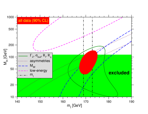
Figure 9: 1$\sigma$ allowed regions in $M_{H}$  vs $m_{t}$  and the 90% cl global fit region from precision data, compared with the direct exclusion limits from LEP 2. Plot courtesy of the Particle Data Group [5].

It is interesting to compare the $Z$ boson couplings measured at different energy scales. The renormalized weak angle measured at different scales in the $\overline{\rm{MS}}$ scheme is displayed in Figure 10.

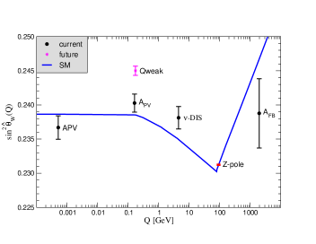
Figure 10: Running $\hat{s}_{Z}^{2}(Q^{2})$ measured at various scales, compared with the predictions of the SM [86]. The low energy points are from atomic parity violation (APV), the polarized Møller asymmetry (PV) and deep inelastic neutrino scattering (corrected for an $s-\bar{s}$ asymmetry). $Q_{weak}$ shows the expected sensitivity of a future polarized $e^{-}$ measurement at Jefferson Lab. Plot courtesy of the Particle Data Group [5].

The precision program has also been used to search for and constrain the effects of possible new TeV scale physics. This includes the effects of possible mixing between ordinary and exotic heavy fermions [68], new $W^{\prime}$ or $Z^{\prime}$ gauge bosons [88, 89], leptoquarks [90, 91, 92, 80], Kaluza-Klein excitations in extra-dimensional theories [93, 94, 95, 5], and new four-fermion operators [96, 90, 97, 80], all of which can effect the observables at tree level. The oblique corrections [98, 99], which only affect the $W$ and $Z$ self energies, are also constrained. The latter may be generated, e.g., by heavy non-degenerate scalar or fermion multiplets and heavy chiral fermions [5], such as are often found in models that replace the elementary Higgs by a dynamical mechanism [100]. A major implication of supersymmetry is through the small mass expected for the lightest Higgs boson. Other supersymmetric effects are small in the decoupling limit in which the superpartners and extra Higgs doublet are heavier than a few hundred GeV [101, 84, 85, 102]. The precisely measured gauge couplings at the $Z$-pole are also important for testing the ideas of gauge coupling unification [103], which works extremely well in the MSSM [104, 105, 106, 107].

4.5 Gauge Self-interactions

The $SU(2)$ gauge kinetic energy terms in (6) lead to 3 and 4-point gauge self-interactions for the $W$’s,

$$\begin{split}\mathcal{L}_{W3}=&-ig\bigl{(}\partial_{\rho}W^{3}_{\nu}\bigr{)}W^{+}_{\mu}W^{-}_{\sigma}\bigl{[}g^{\rho\mu}g^{\nu\sigma}-g^{\rho\sigma}g^{\nu\mu}\bigr{]}\\ &-ig\bigl{(}\partial_{\rho}W^{+}_{\mu}\bigr{)}W^{3}_{\nu}W^{-}_{\sigma}\bigl{[}g^{\rho\sigma}g^{\mu\nu}-g^{\rho\nu}g^{\mu\sigma}\bigr{]}\\ &-ig\bigl{(}\partial_{\rho}W^{-}_{\sigma}\bigr{)}W^{3}_{\nu}W^{+}_{\mu}\bigl{[}g^{\rho\nu}g^{\mu\sigma}-g^{\rho\mu}g^{\nu\sigma}\bigr{]},\end{split}$$ (59)

and

$$\mathcal{L}_{W4}=\frac{g^{2}}{4}\left[W^{+}_{\mu}W^{+}_{\nu}W^{-}_{\sigma}W^{-}_{\rho}{\cal Q}^{\mu\nu\rho\sigma}-2W^{+}_{\mu}W^{3}_{\nu}W^{3}_{\sigma}W^{-}_{\rho}{\cal Q}^{\mu\rho\nu\sigma}\right],$$ (60)

where

$${\cal Q}_{\mu\nu\rho\sigma}\equiv 2g_{\mu\nu}g_{\rho\sigma}-g_{\mu\rho}g_{\nu\sigma}-g_{\mu\sigma}g_{\nu\rho}.$$ (61)

These carry over to the $W$, $Z$, and $\gamma$ self-interactions provided we replace $W^{3}$ by $\cos\theta_{W}Z+\sin\theta_{W}A$ using (26) and (27) (the $B$ has no self-interactions). The resulting vertices follow from the matrix element of $i\mathcal{L}$ after including identical particle factors and using $g=e/\sin\theta_{W}$. They are listed in Table 3 and shown in Figure 11.

$$ie{\cal C}_{\mu\nu\sigma}(p,q,r)$$

$$\begin{split}&{\cal C}_{\mu\nu\sigma}(p,q,r)\equiv g_{\mu\nu}(q-p)_{\sigma}\\ &\quad+g_{\mu\sigma}(p-r)_{\nu}+g_{\nu\sigma}(r-q)_{\mu}\end{split}$$

$$i\frac{e}{\tan\theta_{W}}{\cal C}_{\mu\nu\sigma}(p,q,r)$$

$$i\frac{e^{2}}{\sin^{2}\theta_{W}}{\cal Q}_{\mu\nu\rho\sigma}$$

$$\begin{split}{\cal Q}_{\mu\nu\rho\sigma}\equiv&2g_{\mu\nu}g_{\rho\sigma}\\ &-g_{\mu\rho}g_{\nu\sigma}-g_{\mu\sigma}g_{\nu\rho}\end{split}$$

$$-i\frac{e^{2}}{\tan\theta_{W}}{\cal Q}_{\mu\rho\nu\sigma}$$

$$-i\frac{e^{2}}{\tan^{2}\theta_{W}}{\cal Q}_{\mu\rho\nu\sigma}$$

$$-ie^{2}{\cal Q}_{\mu\rho\nu\sigma}$$

Figure 11: The three and four point-self-interactions of gauge bosons in the standard electroweak model. The momenta and charges flow into the vertices.

The gauge self-interactions are essential probes of the structure and consistency of a spontaneously-broken non-abelian gauge theory. Even tiny deviations in their form or value would destroy the delicate cancellations needed for renormalizability, and would signal the need either for compensating new physics (e.g., from mixing with other gauge bosons or new particles in loops), or of a more fundamental breakdown of the gauge principle, e.g., from some forms of compositeness. They have been constrained by measuring the total cross section and various decay distributions for $e^{-}e^{+}\rightarrow W^{-}W^{+}$ at LEP 2, and by observing $\bar{p}p\rightarrow W^{+}W^{-},WZ,$ and $W\gamma$ at the Tevatron. Possible anomalies in the predicted quartic vertices in Table 3, and the neutral cubic vertices for $ZZZ,$ $ZZ\gamma,$ and $Z\gamma\gamma$, which are absent in the SM, have also been constrained by LEP 2 [80].

The three tree-level diagrams for $e^{-}e^{+}\rightarrow W^{-}W^{+}$ are shown in Figure 12. The cross section from any one or two of these rises rapidly with center of mass energy, but gauge invariance relates these three-point vertices to the couplings of the fermions in such a way that at high energies there is a cancellation. It is another manifestation of the cancellation in a gauge theory which brings higher-order loop integrals under control, leading to a renormalizable theory. It is seen in Figure 13 that the expected cancellations do occur.

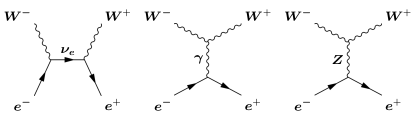
Figure 12: Tree-level diagrams contributing to $e^{+}e^{-}\rightarrow W^{+}W^{-}$.

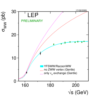
Figure 13: Cross section for $e^{-}e^{+}\rightarrow W^{-}W^{+}$ compared with the SM expectation. Also shown is the expectation from $t$ channel $\nu_{e}$ exchange only, and for the $\nu_{e}$ and $\gamma$ diagrams only. Plot courtesy of the LEP Electroweak Working Group [80], http://www.cern.ch/LEPEWWG/.

5 Problems with the Standard Model

For convenience we summarize the Lagrangian density after spontaneous symmetry breaking:

$$\begin{split}\mathcal{L}&=\mathcal{L}_{gauge}+\mathcal{L}_{\phi}+\sum_{r}\bar{\psi}_{r}\left(i\not{\!\partial}-m_{r}-\frac{m_{r}H}{\nu}\right)\psi_{r}\\ &-\frac{g}{2\sqrt{2}}\left(J^{\mu}_{W}W^{-}_{\mu}+J^{\mu{\dagger}}_{W}W^{+}_{\mu}\right)-eJ^{\mu}_{Q}A_{\mu}-\frac{g}{2\cos\theta_{W}}J^{\mu}_{Z}Z_{\mu},\end{split}$$ (62)

where the self-interactions for the $W^{\pm}$, $Z$, and $\gamma$ are given in (59) and (60), $\mathcal{L}_{\phi}$ is given in (34), and the fermion currents in (43), (50), and (55). For Majorana $\nu_{L}$ masses generated by a higher dimensional operator involving two factors of the Higgs doublet, as in the seesaw model, the $\nu$ term in (62) is replaced by

$$\mathcal{L}=\sum_{r}\bar{\nu}_{rL}i\not{\!\partial}\nu_{rL}-\frac{1}{2}m_{\nu r}\Bigl{(}\bar{\nu}_{rL}\nu^{c}_{rR}+h.c.\Bigr{)}\Bigl{(}1+\frac{H}{\nu}\Bigr{)}^{2},$$ (63)

where $\nu^{c}_{rR}$ is the $CP$ conjugate to $\nu_{L}$ (see, e.g., Langacker:2005pfa).

The standard electroweak model is a mathematically-consistent renormalizable field theory which predicts or is consistent with all experimental facts. It successfully predicted the existence and form of the weak neutral current, the existence and masses of the $W$ and $Z$ bosons, and the charm quark, as necessitated by the GIM mechanism. The charged current weak interactions, as described by the generalized Fermi theory, were successfully incorporated, as was quantum electrodynamics. The consistency between theory and experiment indirectly tested the radiative corrections and ideas of renormalization and allowed the successful prediction of the top quark mass. Although the original formulation did not provide for massive neutrinos, they are easily incorporated by the addition of right-handed states $\nu_{R}$ (Dirac) or as higher-dimensional operators, perhaps generated by an underlying seesaw (Majorana). When combined with quantum chromodynamics for the strong interactions, the standard model is almost certainly the approximately correct description of the elementary particles and their interactions down to at least $10^{-16}$cm, with the possible exception of the Higgs sector or new very weakly coupled particles. When combined with general relativity for classical gravity the SM accounts for most of the observed features of Nature (though not for the dark matter and energy).

However, the theory has far too much arbitrariness to be the final story. For example, the minimal version of the model has 20 free parameters for massless neutrinos and another 7 (9) for massive Dirac (Majorana) neutrinos, not counting electric charge (i.e., hypercharge) assignments. Most physicists believe that this is just too much for the fundamental theory. The complications of the standard model can also be described in terms of a number of problems.

The Gauge Problem

The standard model is a complicated direct product of three subgroups, $SU(3)\times SU(2)\times U(1)$, with separate gauge couplings. There is no explanation for why only the electroweak part is chiral (parity-violating). Similarly, the standard model incorporates but does not explain another fundamental fact of nature: charge quantization, i.e., why all particles have charges which are multiples of $e/3$. This is important because it allows the electrical neutrality of atoms $(|q_{p}|=|q_{e}|)$. The complicated gauge structure suggests the existence of some underlying unification of the interactions, such as one would expect in a superstring [108, 109, 110] or grand unified theory [111, 112, 113, 88, 114]. Charge quantization can also be explained in such theories, though the “wrong” values of charge emerge in some constructions due to different hypercharge embeddings or non-canonical values of $Y$ (e.g., some string constructions lead to exotic particles with charges of $\pm e/2$). Charge quantization may also be explained, at least in part, by the existence of magnetic monopoles [115] or the absence of anomalies, but either of these is likely to find its origin in some kind of underlying unification.

The Fermion Problem

All matter under ordinary terrestrial conditions can be constructed out of the fermions $(\nu_{e},e^{-},u,d)$ of the first family. Yet we know from laboratory studies that there are $\geq 3$ families: $(\nu_{\mu},\mu^{-},c,s)$ and $(\nu_{\tau},\tau^{-},t,b)$ are heavier copies of the first family with no obvious role in nature. The standard model gives no explanation for the existence of these heavier families and no prediction for their numbers. Furthermore, there is no explanation or prediction of the fermion masses, which are observed to occur in a hierarchical pattern which varies over 5 orders of magnitude between the $t$ quark and the $e^{-}$, or of the quark and lepton mixings. Even more mysterious are the neutrinos, which are many orders of magnitude lighter still. It is not even certain whether the neutrino masses are Majorana or Dirac. A related difficulty is that while the $CP$ violation observed in the laboratory is well accounted for by the phase in the CKM matrix, there is no SM source of $CP$ breaking adequate to explain the baryon asymmetry of the universe.

There are many possible suggestions of new physics that might shed light on these questions. The existence of multiple families could be due to large representations of some string theory or grand unification, or they could be associated with different possibilities for localizing particles in some higher dimensional space. The latter could also be associated with string compactifications, or by some effective brane world scenario [93, 94, 95, 5]. The hierarchies of masses and mixings could emerge from wave function overlap effects in such higher-dimensional spaces. Another interpretation, also possible in string theories, is that the hierarchies are because some of the mass terms are generated by higher dimensional operators and therefore suppressed by powers of $\langle 0|S|0\rangle/M_{X}$, where $S$ is some standard model singlet field and $M_{X}$ is some large scale such as $M_{P}$. The allowed operators could perhaps be enforced by some family symmetry [116]. Radiative hierarchies [117], in which some of the masses are generated at the loop level, or some form of compositeness are other possibilities. Despite all of these ideas there is no compelling model and none of these yields detailed predictions. Grand unification by itself doesn’t help very much, except for the prediction of $m_{b}$ in terms of $m_{\tau}$ in the simplest versions.

The small values for the neutrino masses suggest that they are associated with Planck or grand unification physics, as in the seesaw model, but there are other possibilities [44, 45, 46, 47].

Almost any type of new physics is likely to lead to new sources of $CP$ violation.

The Higgs/Hierarchy Problem

In the standard model one introduces an elementary Higgs field to generate masses for the $W$, $Z$, and fermions. For the model to be consistent the Higgs mass should not be too different from the $W$ mass. If $M_{H}$ were to be larger than $M_{W}$ by many orders of magnitude the Higgs self-interactions would be excessively strong. Theoretical arguments suggest that $M_{H}\lesssim 700$ GeV (see Section 3).

However, there is a complication. The tree-level (bare) Higgs mass receives quadratically-divergent corrections from the loop diagrams in Figure 14.

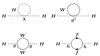
Figure 14: Radiative corrections to the Higgs mass, including self-interactions, interactions with gauge bosons, and interactions with fermions.

One finds

$$M_{H}^{2}=(M_{H}^{2})_{bare}+{\cal O}(\lambda,g^{2},h^{2})\Lambda^{2},$$ (64)

where $\Lambda$ is the next higher scale in the theory. If there were no higher scale one could simply interpret $\Lambda$ as an ultraviolet cutoff and take the view that $M_{H}$ is a measured parameter, with $(M_{H})_{bare}$ not observable. However, the theory is presumably embedded in some larger theory that cuts off the momentum integral at the finite scale of the new physics. For example, if the next scale is gravity $\Lambda$ is the Planck scale $M_{P}=G_{N}^{-1/2}\sim 10^{19}$ GeV. In a grand unified theory, one would expect $\Lambda$ to be of order the unification scale $M_{X}\sim 10^{14}$ GeV. Hence, the natural scale for $M_{H}$ is ${\cal O}(\Lambda)$, which is much larger than the expected value. There must be a fine-tuned and apparently highly contrived cancellation between the bare value and the correction, to more than 30 decimal places in the case of gravity. If the cutoff is provided by a grand unified theory there is a separate hierarchy problem at the tree-level. The tree-level couplings between the Higgs field and the superheavy fields lead to the expectation that $M_{H}$ is close to the unification scale unless unnatural fine-tunings are done, i.e., one does not understand why $(M_{W}/M_{X})^{2}$ is so small in the first place.

One solution to this Higgs/hierarchy problem is TeV scale supersymmetry, in which the quadratically-divergent contributions of fermion and boson loops cancel, leaving only much smaller effects of the order of supersymmetry-breaking. (However, supersymmetric grand unified theories still suffer from the tree-level hierarchy problem.) There are also (non-supersymmetric) extended models in which the cancellations are between bosons or between fermions. This class includes Little Higgs models [118, 119], in which the Higgs is forced to be lighter than new TeV scale dynamics because it is a pseudo-Goldstone boson of an approximate underlying global symmetry, and Twin-Higgs models [120].

Another possibility is to eliminate the elementary Higgs fields, replacing them with some dynamical symmetry breaking mechanism based on a new strong dynamics [100]. In technicolor, for example, the SSB is associated with the expectation value of a fermion bilinear, analogous to the breaking of chiral symmetry in QCD. Extended technicolor, top-color, and composite Higgs models all fall into this class.

Large and/or warped extra dimensions [121, 122, 123] can also resolve the difficulties, by altering the relation between $M_{P}$ and a much lower fundamental scale, by providing a cutoff at the inverse of the extra dimension scale, or by using the boundary conditions in the extra dimensions to break the electroweak symmetry (Higgsless models [124]). Deconstruction models, in which no extra dimensions are explicity introduced [125, 126], are closely related.

Most of the models mentioned above have the potential to generate flavor changing neutral current and $CP$ violation effects much larger than observational limits. Pushing the mass scales high enough to avoid these problems may conflict with a natural solution to the hierarchy problem, i.e., one may reintroduce a little hierarchy problem. Many are also strongly constrained by precision electroweak physics. In some cases the new physics does not satisfy the decoupling theorem [127], leading to large oblique corrections. In others new tree-level effects may again force the scale to be too high. The most successful from the precision electroweak point of view are those which have a discrete symmetry which prevents vertices involving just one heavy particle, such as $R$-parity in supersymmetry, $T$-parity in some little Higgs models [128], and $KK$-parity in universal extra dimension models [129].

A very different possibility is to accept the fine-tuning, i.e., to abandon the notion of naturalness for the weak scale, perhaps motivated by anthropic considerations [130]. (The anthropic idea will be considered below in the discussion of the gravity problem.) This could emerge, for example, in split supersymmetry [131].

The Strong $CP$ Problem

Another fine-tuning problem is the strong $CP$ problem [132, 133, 134]. One can add an additional term $\frac{\theta_{QCD}}{32\pi^{2}}g^{2}_{s}G\tilde{G}$ to the QCD Lagrangian density which breaks $P$, $T$ and $CP$ symmetry. $\tilde{G}_{\mu\nu}^{i}=\epsilon_{\mu\nu\alpha\beta}G^{\alpha\beta i}/2$ is the dual field strength tensor. This term, if present, would induce an electric dipole moment $d_{N}$ for the neutron. The rather stringent limits on the dipole moment lead to the upper bound $|\theta_{QCD}|<10^{-11}$. The question is, therefore, why is $\theta_{QCD}$ so small? It is not sufficient to just say that it is zero (i.e., to impose $CP$ invariance on QCD) because of the observed violation of $CP$ by the weak interactions. As discussed in Section 4.1, this is believed to be associated with phases in the quark mass matrices. The quark phase redefinitions which remove them lead to a shift in $\theta_{QCD}$ by $\mathcal{O}(10^{-3})$ because of the anomaly in the vertex coupling the associated global current to two gluons. Therefore, an apparently contrived fine-tuning is needed to cancel this correction against the bare value. Solutions include the possibility that $CP$ violation is not induced directly by phases in the Yukawa couplings, as is usually assumed in the standard model, but is somehow violated spontaneously. $\theta_{QCD}$ then would be a calculable parameter induced at loop level, and it is possible to make $\theta_{QCD}$ sufficiently small. However, such models lead to difficult phenomenological and cosmological problems. Alternately, $\theta_{QCD}$ becomes unobservable (i.e., can be rotated away) if there is a massless $u$ quark [138]. However, most phenomenological estimates [139] are not consistent with $m_{u}=0$. Another possibility is the Peccei-Quinn mechanism [140], in which an extra global $U(1)$ symmetry is imposed on the theory in such a way that $\theta_{QCD}$ becomes a dynamical variable which is zero at the minimum of the potential. The spontaneous breaking of the symmetry, along with explicit breaking associated with the anomaly and instanton effects, leads to a very light pseudo-Goldstone boson known as an axion [141, 142]. Laboratory, astrophysical, and cosmological constraints suggest the range $10^{9}-10^{12}$ GeV for the scale at which the $U(1)$ symmetry is broken.

The Gravity Problem

Gravity is not fundamentally unified with the other interactions in the standard model, although it is possible to graft on classical general relativity by hand. However, general relativity is not a quantum theory, and there is no obvious way to generate one within the standard model context. Possible solutions include Kaluza-Klein [143] and supergravity [144, 145, 146] theories. These connect gravity with the other interactions in a more natural way, but do not yield renormalizable theories of quantum gravity. More promising are superstring theories (which may incorporate the above), which unify gravity and may yield finite theories of quantum gravity and all the other interactions. String theories are perhaps the most likely possibility for the underlying theory of particle physics and gravity, but at present there appear to be a nearly unlimited number of possible string vacua (the landscape), with no obvious selection principle. As of this writing the particle physics community is still trying to come to grips with the landscape and its implications. Superstring theories naturally imply some form of supersymmetry, but it could be broken at a high scale and have nothing to do with the Higgs/hierarachy problem (split supersymmetry is a compromise, keeping some aspects at the TeV scale).

In addition to the fact that gravity is not unified and not quantized there is another difficulty, namely the cosmological constant. The cosmological constant can be thought of as the energy of the vacuum. However, we saw in Section 3 that the spontaneous breaking of $SU(2)\times U(1)$ generates a value $\langle 0|V(\nu)|0\rangle=-\mu^{4}/4\lambda$ for the expectation value of the Higgs potential at the minimum. This is a $c$-number which has no significance for the microscopic interactions. However, it assumes great importance when the theory is coupled to gravity, because it contributes to the cosmological constant. The cosmological constant becomes

$$\Lambda_{cosm}=\Lambda_{bare}+\Lambda_{SSB},$$ (65)

where $\Lambda_{bare}=8\pi G_{N}V(0)$ is the primordial cosmological constant, which can be thought of as the value of the energy of the vacuum in the absence of spontaneous symmetry breaking. (The definition of $V(\phi)$ in (10) implicitly assumed $\Lambda_{bare}=0$.) $\Lambda_{SSB}$ is the part generated by the Higgs mechanism:

$$|\Lambda_{SSB}|=8\pi G_{N}|\langle 0|V|0\rangle|\sim 10^{56}\Lambda_{obs}.$$ (66)

It is some $10^{56}$ times larger in magnitude than the observed value $\Lambda_{obs}\sim(0.0024\text{ eV})^{4}/8\pi G_{N}$ (assuming that the dark energy is due to a cosmological constant), and it is of the wrong sign.

This is clearly unacceptable. Technically, one can solve the problem by adding a constant $+\mu^{4}/4\lambda$ to $V$, so that $V$ is equal to zero at the minimum (i.e., $\Lambda_{bare}=2\pi G_{N}\mu^{4}/\lambda)$. However, with our current understanding there is no reason for $\Lambda_{bare}$ and $\Lambda_{SSB}$ to be related. The need to invoke such an incredibly fine-tuned cancellation to 50 decimal places is probably the most unsatisfactory feature of the standard model. The problem becomes even worse in superstring theories, where one expects a vacuum energy of ${\cal O}(M_{P}^{4})$ for a generic point in the landscape, leading to $\Lambda_{obs}\gtrsim 10^{123}|\Lambda_{obs}|$. The situation is almost as bad in grand unified theories.

So far no compelling solution to the cosmological constant problem has emerged. One intriguing possibility invokes the anthropic (environmental) principle [147, 148, 149], i.e., that a much larger or smaller value of $|\Lambda_{cosm}|$ would not have allowed the possibility for life to have evolved because the Universe would have expanded or recollapsed too rapidly [150]. This would be a rather meaningless argument unless (a) Nature somehow allows a large variety of possibilities for $|\Lambda_{cosm}|$ (and possibly other parameters or principles) such as in different vacua, and (b) there is some mechanism to try all or many of them. In recent years it has been suggested that both of these needs may be met. There appear to be an enormous landscape of possible superstring vacua [151, 152, 153, 154], with no obvious physical principle to choose one over the other. Something like eternal inflation [155] could provide the means to sample them, so that only the environmentally suitable vacua lead to long-lived Universes suitable for life. These ideas are highly controversial and are currently being heatedly debated.

The New Ingredients

It is now clear that the standard model requires a number of new ingredients. These include

• A mechanism for small neutrino masses. The most popular possibility is the minimal seesaw model, implying Majorana masses, but there are other plausible mechanisms for either small Dirac or Majorana masses [44, 45, 46, 47].

• A mechanism for the baryon asymmetry. The standard model has neither the nonequilibrium condition nor sufficient $CP$ violation to explain the observed asymmetry between baryons and antibaryons in the Universe [156, 157, 158]. One possibility involves the out of equilibrium decays of superheavy Majorana right-handed neutrinos (leptogenesis [162, 163]), as expected in the minimal seesaw model. Another involves a strongly first order electroweak phase transition (electroweak baryogenesis [164]). This is not expected in the standard model, but could possibly be associated with loop effects in the minimal supersymmetric extension (MSSM) if one of the scalar top quarks is sufficiently light [165]. However, it is most likely in extensions of the MSSM involving SM singlet Higgs fields that can generate a dynamical $\mu$ term, which can easily lead to strong first order transitions at tree-level [166]. Such extensions would likely yield signatures observable at the LHC. Both the seesaw models and the singlet extensions of the MSSM could also provide the needed new sources of $CP$ violation. Other possibilities for the baryon asymmetry include the decay of a coherent scalar field, such as a scalar quark or lepton in supersymmetry (the Affleck-Dine mechanism [167]), or $CPT$ violation [168, 169]. Finally, one cannot totally dismiss the possibility that the asymmetry is simply due to an initial condition on the big bang. However, this possibility disappears if the universe underwent a period of rapid inflation [170].

• What is the dark energy? In recent years a remarkable concordance of cosmological observations involving the cosmic microwave background radiation (CMB), acceleration of the Universe as determined by Type Ia supernova observations, large scale distribution of galaxies and clusters, and big bang nucleosynthesis has allowed precise determinations of the cosmological parameters [171, 172, 173, 5]: the Universe is close to flat, with some form of dark energy making up about 74% of the energy density. Dark matter constitutes $\gtrsim 21$%, while ordinary matter (mainly baryons) represents only about 4-5%. The mysterious dark energy [174, 175, 176], which is the most important contribution to the energy density and leads to the acceleration of the expansion of the Universe, is not accounted for in the SM. It could be due to a cosmological constant that is incredibly tiny on the particle physics scale, or to a slowly time varying field (quintessence). Is the acceleration somehow related to an earlier and much more dramatic period of inflation [170]? If it is associated with a time-varying field, could it be connected with a possible time variation of coupling “constants” [177]?

• What is the dark matter? Similarly, the standard model has no explanation for the observed dark matter, which contributes much more to the matter in the Universe than the stuff we are made of. It is likely, though not certain, that the dark matter is associated with elementary particles. An attractive possibility is weakly interacting massive particles (WIMPs), which are typically particles in the $10^{2}-10^{3}$ GeV range with weak interaction strength couplings, and which lead naturally to the observed matter density. These could be associated with the lightest supersymmetric partner (usually a neutralino) in supersymmetric models with $R$-parity conservation, or analogous stable particles in Little Higgs or universal extra dimension models. There are a wide variety of variations on these themes, e.g., involving very light gravitinos or other supersymmetric particles. There are many searches for WIMPs going on, including direct searches for the recoil produced by scattering of Solar System WIMPs, indirect searches for WIMP annihilation products, and searches for WIMPs produced at accelerators [178, 179, 180]. Axions, perhaps associated with the strong $CP$ problem or with string vacua [181], are another possibility. Searches for axions produced in the Sun, in the laboratory, or from the early universe are currently underway [182, 134].

• The suppression of flavor changing neutral currents, proton decay, and electric dipole moments. The standard model has a number of accidental symmetries and features which forbid proton decay, preserve lepton number and lepton family number (at least for vanishing neutrino masses), suppress transitions such as $K^{+}\rightarrow\pi^{+}\nu\bar{\nu}$ at tree-level, and lead to highly suppressed electric dipole moments for the $e^{-}$, $n$, atoms, etc. However, most extensions of the SM have new interactions which violate such symmetries, leading to potentially serious problems with FCNC and EDMs. There seems to be a real conflict between attempts to deal with the Higgs/hierarchy problem and the prevention of such effects.

  Recently, there has been much discussion of minimal flavor violation, which is the hypothesis that all flavor violation, even that which is associated with new physics, is proportional to the standard model Yukawa matrices [183, 51], leading to a significant suppression of flavor changing effects.

References

- [1] H. Weyl, Z. Phys. 56, 330 (1929).
- [2] C.-N. Yang and R. L. Mills, Phys. Rev. 96, 191 (1954).
- [3] D. J. Gross, Rev. Mod. Phys. 77, 837 (2005).
- [4] S. Bethke, Prog. Part. Nucl. Phys. 58, 351 (2007).
- [5] C. Amsler et al., Phys. Lett. B667, p. 1 (2008).
- [6] D. J. Gross and F. Wilczek, Phys. Rev. Lett. 30, 1343 (1973).
- [7] H. D. Politzer, Phys. Rev. Lett. 30, 1346 (1973).
- [8] H. Fritzsch, M. Gell-Mann and H. Leutwyler, Phys. Lett. B47, 365 (1973).
- [9] J. Gasser and H. Leutwyler, Phys. Rept. 87, 77 (1982).
- [10] S. L. Glashow, Nucl. Phys. 22, 579 (1961).
- [11] S. Weinberg, Phys. Rev. Lett. 19, 1264 (1967).
- [12] A. Salam In Elementary Particle Theory, ed. N. Svartholm (Almquist and Wiksells, Stockholm 1969), 367-377.
- [13] J. S. Schwinger, Phys. Rev. 125, 397 (1962).
- [14] P. W. Anderson, Phys. Rev. 130, 439 (1963).
- [15] P. W. Higgs, Phys. Lett. 12, 132 (1964).
- [16] P. W. Higgs, Phys. Rev. 145, 1156 (1966).
- [17] F. Englert and R. Brout, Phys. Rev. Lett. 13, 321 (1964).
- [18] G. S. Guralnik, C. R. Hagen and T. W. B. Kibble, Phys. Rev. Lett. 13, 585 (1964).
- [19] G. ’t Hooft, Nucl. Phys. B35, 167 (1971).
- [20] G. ’t Hooft and M. J. G. Veltman, Nucl. Phys. B50, 318 (1972).
- [21] B. W. Lee and J. Zinn-Justin, Phys. Rev. D5, 3121 (1972).
- [22] B. W. Lee and J. Zinn-Justin, Phys. Rev. D7, 1049 (1973).
- [23] S. R. Coleman, Aspects of symmetry: selected Erice lectures (Cambridge Univ. Press, Cambridge, 1985).
- [24] A. Vilenkin, Phys. Rept. 121, p. 263 (1985).
- [25] S. R. Coleman and E. Weinberg, Phys. Rev. D7, 1888 (1973).
- [26] T. W. B. Kibble, Phys. Rev. 155, 1554 (1967).
- [27] Y. Nambu, Phys. Rev. Lett. 4, 380 (1960).
- [28] Y. Nambu and G. Jona-Lasinio, Phys. Rev. 122, 345 (1961).
- [29] J. Goldstone, Nuovo Cim. 19, 154 (1961).
- [30] J. Goldstone, A. Salam and S. Weinberg, Phys. Rev. 127, 965 (1962).
- [31] G. Arnison et al., Phys. Lett. B166, p. 484 (1986).
- [32] R. Ansari et al., Phys. Lett. B186, p. 440 (1987).
- [33] R. Barate et al., Phys. Lett. B565, 61 (2003).
- [34] N. Cabibbo, L. Maiani, G. Parisi and R. Petronzio, Nucl. Phys. B158, p. 295 (1979).
- [35] J. F. Gunion, S. Dawson, H. E. Haber and G. L. Kane, The Higgs hunter’s guide (Westview, Boulder, CO, 1990).
- [36] T. Hambye and K. Riesselmann (1997), hep-ph/9708416.
- [37] A. Hasenfratz, K. Jansen, C. B. Lang, T. Neuhaus and H. Yoneyama, Phys. Lett. B199, p. 531 (1987).
- [38] J. Kuti, L. Lin and Y. Shen, Phys. Rev. Lett. 61, p. 678 (1988).
- [39] M. Luscher and P. Weisz, Nucl. Phys. B318, p. 705 (1989).
- [40] B. W. Lee, C. Quigg and H. B. Thacker, Phys. Rev. D16, p. 1519 (1977).
- [41] G. Altarelli and G. Isidori, Phys. Lett. B337, 141 (1994).
- [42] J. A. Casas, J. R. Espinosa and M. Quiros, Phys. Lett. B382, 374 (1996).
- [43] G. Isidori, G. Ridolfi and A. Strumia, Nucl. Phys. B609, 387 (2001).
- [44] M. C. Gonzalez-Garcia and Y. Nir, Rev. Mod. Phys. 75, 345 (2003).
- [45] P. Langacker, J. Erler and E. Peinado, J. Phys. Conf. Ser. 18, 154 (2005).
- [46] R. N. Mohapatra et al., Rept. Prog. Phys. 70, 1757 (2007).
- [47] M. C. Gonzalez-Garcia and M. Maltoni, Phys. Rept. 460, 1 (2008).
- [48] S. L. Glashow and S. Weinberg, Phys. Rev. D15, p. 1958 (1977).
- [49] M. K. Gaillard and B. W. Lee, Phys. Rev. D10, p. 897 (1974).
- [50] P. Langacker (1991), in TeV Physics, ed T. Huang et al., Gordon and Breach, N.Y., 1991.
- [51] Y. Nir (2007), 0708.1872.
- [52] N. Cabibbo, Phys. Rev. Lett. 10, 531 (1963).
- [53] M. Kobayashi and T. Maskawa, Prog. Theor. Phys. 49, 652 (1973).
- [54] L. Wolfenstein, Phys. Rev. Lett. 51, p. 1945 (1983).
- [55] E. D. Commins and P. H. Bucksbaum, Weak interactions of leptons and quarks (Cambridge Univ. Press, Cambridge, 1983).
- [56] P. B. Renton, Electroweak interactions (Cambridge Univ. Press, Cambridge, 1990).
- [57] P. G. Langacker, Precision tests of the standard electroweak model (World Scientific, Singapore, 1995).
- [58] A. Czarnecki, W. J. Marciano and A. Sirlin, Phys. Rev. D70, p. 093006 (2004).
-
[59]
J. Charles et al., Eur. Phys. J. C41, 1 (2005), with updated
results and plots available at:
http://ckmfitter.in2p3.fr. - [60] T. Kinoshita, Quantum electrodynamics (World Scientific, Singapore, 1990).
- [61] S. G. Karshenboim, Phys. Rept. 422, 1 (2005).
- [62] P. J. Mohr, B. N. Taylor and D. B. Newell, Rev. Mod. Phys. 80, 633 (2008).
- [63] S. L. Wu, Phys. Rept. 107, 59 (1984).
- [64] C. Kiesling, Tests of the standard theory of electroweak interactions (Springer, Berlin, 1988).
- [65] G. W. Bennett et al., Phys. Rev. D73, p. 072003 (2006).
- [66] A. Czarnecki and W. J. Marciano, Phys. Rev. D64, p. 013014 (2001).
- [67] S. L. Glashow, J. Iliopoulos and L. Maiani, Phys. Rev. D2, 1285 (1970).
- [68] P. Langacker and D. London, Phys. Rev. D38, p. 886 (1988).
- [69] F. J. Hasert et al., Phys. Lett. B46, 138 (1973).
- [70] A. C. Benvenuti and e. al., Phys. Rev. Lett. 32, 800 (1974).
- [71] J. E. Kim, P. Langacker, M. Levine and H. H. Williams, Rev. Mod. Phys. 53, p. 211 (1981).
- [72] U. Amaldi et al., Phys. Rev. D36, p. 1385 (1987).
- [73] G. Costa, J. R. Ellis, G. L. Fogli, D. V. Nanopoulos and F. Zwirner, Nucl. Phys. B297, p. 244 (1988).
- [74] P. Langacker, M.-x. Luo and A. K. Mann, Rev. Mod. Phys. 64, 87 (1992).
- [75] J. Erler and P. Langacker (2008), 0807.3023.
- [76] P. Langacker (1993), hep-ph/9305255.
- [77] G. P. Zeller et al., Phys. Rev. Lett. 88, p. 091802 (2002).
- [78] D. Mason et al., Phys. Rev. Lett. 99, p. 192001 (2007).
- [79] S. Schael et al., Phys. Rept. 427, p. 257 (2006).
- [80] J. Alcaraz et al. (2006), hep-ex/0612034.
- [81] K. Wichmann (2007), 0707.2724.
- [82] K. Maltman and T. Yavin (2008), 0812.2457.
- [83] M. S. Chanowitz, Phys. Rev. D66, p. 073002 (2002).
- [84] S. Heinemeyer, W. Hollik and G. Weiglein, Phys. Rept. 425, 265 (2006).
- [85] S. Heinemeyer, W. Hollik, A. M. Weber and G. Weiglein, JHEP 04, p. 039 (2008).
- [86] A. Czarnecki and W. J. Marciano, Int. J. Mod. Phys. A15, 2365 (2000).
- [87] J. Erler, A. Kurylov and M. J. Ramsey-Musolf, Phys. Rev. D68, p. 016006 (2003).
- [88] J. L. Hewett and T. G. Rizzo, Phys. Rept. 183, p. 193 (1989).
- [89] P. Langacker (2008), 0801.1345.
- [90] K.-m. Cheung, Phys. Lett. B517, 167 (2001).
- [91] M. Chemtob, Prog. Part. Nucl. Phys. 54, 71 (2005).
- [92] R. Barbier et al., Phys. Rept. 420, 1 (2005).
- [93] J. L. Hewett and M. Spiropulu, Ann. Rev. Nucl. Part. Sci. 52, 397 (2002).
- [94] C. Csaki (2004), hep-ph/0404096.
- [95] R. Sundrum (2005), hep-th/0508134.
- [96] G.-C. Cho, K. Hagiwara and S. Matsumoto, Eur. Phys. J. C5, 155 (1998).
- [97] Z. Han and W. Skiba, Phys. Rev. D71, p. 075009 (2005).
- [98] M. E. Peskin and T. Takeuchi, Phys. Rev. Lett. 65, 964 (1990).
- [99] M. E. Peskin and T. Takeuchi, Phys. Rev. D46, 381 (1992).
- [100] C. T. Hill and E. H. Simmons, Phys. Rept. 381, 235 (2003).
- [101] J. Erler and D. M. Pierce, Nucl. Phys. B526, 53 (1998).
- [102] J. R. Ellis, S. Heinemeyer, K. A. Olive, A. M. Weber and G. Weiglein, JHEP 08, p. 083 (2007).
- [103] H. Georgi, H. R. Quinn and S. Weinberg, Phys. Rev. Lett. 33, 451 (1974).
- [104] U. Amaldi, W. de Boer and H. Furstenau, Phys. Lett. B260, 447 (1991).
- [105] J. R. Ellis, S. Kelley and D. V. Nanopoulos, Phys. Lett. B249, 441 (1990).
- [106] C. Giunti, C. W. Kim and U. W. Lee, Mod. Phys. Lett. A6, 1745 (1991).
- [107] P. Langacker and M.-x. Luo, Phys. Rev. D44, 817 (1991).
- [108] M. B. Green, J. H. Schwarz and E. Witten, Superstring theory (Cambridge Univ. Press, New York, NY, 1987).
- [109] J. Polchinski, String Theory (Cambridge Univ. Press, Cambridge, 1998).
- [110] K. Becker, M. Becker and J. Schwarz, String Theory and M-Theory: A Modern Introduction (Cambridge Univ. Press, Cambridge, 2007).
- [111] H. Georgi and S. L. Glashow, Phys. Rev. Lett. 32, 438 (1974).
- [112] P. Langacker, Phys. Rept. 72, p. 185 (1981).
- [113] G. G. Ross, Grand Unified Theories (Westview Press, Reading, MA, 1985).
- [114] S. Raby (2008), 0807.4921.
- [115] J. Preskill, Ann. Rev. Nucl. Part. Sci. 34, 461 (1984).
- [116] C. D. Froggatt and H. B. Nielsen, Nucl. Phys. B147, p. 277 (1979).
- [117] K. S. Babu and R. N. Mohapatra, Phys. Rev. Lett. 66, 556 (1991).
- [118] N. Arkani-Hamed, A. G. Cohen, E. Katz and A. E. Nelson, JHEP 07, p. 034 (2002).
- [119] M. Perelstein, Prog. Part. Nucl. Phys. 58, 247 (2007).
- [120] Z. Chacko, H.-S. Goh and R. Harnik, Phys. Rev. Lett. 96, p. 231802 (2006).
- [121] N. Arkani-Hamed, S. Dimopoulos and G. R. Dvali, Phys. Lett. B429, 263 (1998).
- [122] K. R. Dienes, E. Dudas and T. Gherghetta, Nucl. Phys. B537, 47 (1999).
- [123] L. Randall and R. Sundrum, Phys. Rev. Lett. 83, 3370 (1999).
- [124] C. Csaki, C. Grojean, L. Pilo and J. Terning, Phys. Rev. Lett. 92, p. 101802 (2004).
- [125] N. Arkani-Hamed, A. G. Cohen and H. Georgi, Phys. Lett. B513, 232 (2001).
- [126] C. T. Hill, S. Pokorski and J. Wang, Phys. Rev. D64, p. 105005 (2001).
- [127] T. Appelquist and J. Carazzone, Phys. Rev. D11, p. 2856 (1975).
- [128] H.-C. Cheng and I. Low, JHEP 09, p. 051 (2003).
- [129] T. Appelquist, H.-C. Cheng and B. A. Dobrescu, Phys. Rev. D64, p. 035002 (2001).
- [130] V. Agrawal, S. M. Barr, J. F. Donoghue and D. Seckel, Phys. Rev. D57, 5480 (1998).
- [131] N. Arkani-Hamed and S. Dimopoulos, JHEP 06, p. 073 (2005).
- [132] R. D. Peccei, Adv. Ser. Direct. High Energy Phys. 3, 503 (1989).
- [133] M. Dine (2000), hep-ph/0011376.
- [134] J. E. Kim and G. Carosi (2008), 0807.3125.
- [135] A. A. Anselm and A. A. Johansen, Nucl. Phys. B412, 553 (1994).
- [136] A. E. Nelson, Phys. Lett. B143, p. 165 (1984).
- [137] S. M. Barr, Phys. Rev. D30, p. 1805 (1984).
- [138] D. B. Kaplan and A. V. Manohar, Phys. Rev. Lett. 56, p. 2004 (1986).
- [139] D. R. Nelson, G. T. Fleming and G. W. Kilcup, Phys. Rev. Lett. 90, p. 021601 (2003).
- [140] R. D. Peccei and H. R. Quinn, Phys. Rev. Lett. 38, 1440 (1977).
- [141] S. Weinberg, Phys. Rev. Lett. 40, 223 (1978).
- [142] F. Wilczek, Phys. Rev. Lett. 40, 279 (1978).
- [143] A. Chodos, P. G. O. Freund and T. W. Appelquist, Modern Kaluza-Klein theories (Addison-Wesley, Merlo Park, CA, 1987).
- [144] H. P. Nilles, Phys. Rept. 110, p. 1 (1984).
- [145] J. Wess and J. A. Bagger, Supersymmetry and supergravity (Princeton Univ. Press, Princeton, NJ, 1992).
- [146] J. Terning, Modern Supersymmetry: Dynamics and Duality (Clarendon Press, Oxford, 2006).
- [147] J. D. Barrow and F. J. Tipler, The anthropic cosmological principle (Clarendon Press, Oxford, 1986).
- [148] M. J. Rees (2004), astro-ph/0401424.
- [149] C. J. Hogan, Rev. Mod. Phys. 72, 1149 (2000).
- [150] S. Weinberg, Rev. Mod. Phys. 61, 1 (1989).
- [151] R. Bousso and J. Polchinski, JHEP 06, p. 006 (2000).
- [152] S. Kachru, R. Kallosh, A. Linde and S. P. Trivedi, Phys. Rev. D68, p. 046005 (2003).
- [153] L. Susskind (2003), hep-th/0302219.
- [154] F. Denef and M. R. Douglas, JHEP 05, p. 072 (2004).
- [155] A. D. Linde, Mod. Phys. Lett. A1, p. 81 (1986).
- [156] A. D. Sakharov, JETP Lett. 5, 24 (1967).
- [157] W. Bernreuther, Lect. Notes Phys. 591, 237 (2002).
- [158] M. Dine and A. Kusenko, Rev. Mod. Phys. 76, p. 1 (2004).
- [159] G. ’t Hooft, Phys. Rev. Lett. 37, 8 (1976).
- [160] F. R. Klinkhamer and N. S. Manton, Phys. Rev. D30, p. 2212 (1984).
- [161] V. A. Kuzmin, V. A. Rubakov and M. E. Shaposhnikov, Phys. Lett. B155, p. 36 (1985).
- [162] M. Fukugita and T. Yanagida, Phys. Lett. B174, p. 45 (1986).
- [163] S. Davidson, E. Nardi and Y. Nir, Phys. Rept. 466, 105 (2008).
- [164] M. Trodden, Rev. Mod. Phys. 71, 1463 (1999).
- [165] M. Carena, G. Nardini, M. Quiros and C. E. M. Wagner, JHEP 10, p. 062 (2008).
- [166] V. Barger, P. Langacker and G. Shaughnessy, New J. Phys. 9, p. 333 (2007).
- [167] I. Affleck and M. Dine, Nucl. Phys. B249, p. 361 (1985).
- [168] A. G. Cohen and D. B. Kaplan, Phys. Lett. B199, p. 251 (1987).
- [169] H. Davoudiasl, R. Kitano, G. D. Kribs, H. Murayama and P. J. Steinhardt, Phys. Rev. Lett. 93, p. 201301 (2004).
- [170] D. H. Lyth and A. Riotto, Phys. Rept. 314, 1 (1999).
- [171] E. W. Kolb and M. S. Turner, The early universe (Addison-Wesley, Redwood City, CA, 1990).
- [172] P. J. E. Peebles, Principles of physical cosmology (Princeton Univ. Press, Princeton, NJ, 1993).
- [173] J. Dunkley et al. (2008), 0803.0586.
- [174] P. J. E. Peebles and B. Ratra, Rev. Mod. Phys. 75, 559 (2003).
- [175] J. Frieman, M. Turner and D. Huterer (2008), 0803.0982.
- [176] J. Martin, Mod. Phys. Lett. A23, 1252 (2008).
- [177] J.-P. Uzan, Rev. Mod. Phys. 75, p. 403 (2003).
- [178] G. Jungman, M. Kamionkowski and K. Griest, Phys. Rept. 267, 195 (1996).
- [179] G. Bertone, D. Hooper and J. Silk, Phys. Rept. 405, 279 (2005).
- [180] D. Hooper and E. A. Baltz, Ann. Rev. Nucl. Part. Sci. 58, 293 (2008).
- [181] P. Svrcek and E. Witten, JHEP 06, p. 051 (2006).
- [182] S. J. Asztalos, L. J. Rosenberg, K. van Bibber, P. Sikivie and K. Zioutas, Ann. Rev. Nucl. Part. Sci. 56, 293 (2006).
- [183] G. D’Ambrosio, G. F. Giudice, G. Isidori and A. Strumia, Nucl. Phys. B645, 155 (2002).