Deep-Sea Acoustic Neutrino Detection and the AMADEUS System as a Multi-Purpose Acoustic Array

Abstract

The use of conventional neutrino telescope methods and technology for detecting neutrinos with energies above 1 EeV from astrophysical sources would be prohibitively expensive and may turn out to be technically not feasible. Acoustic detection is a promising alternative for future deep-sea neutrino telescopes operating in this energy regime. It utilises the effect that the energy deposit of the particle cascade evolving from a neutrino interaction in water generates a coherently emitted sound wave with frequency components in the range between about 1 and 50 kHz. The AMADEUS (Antares Modules for Acoustic DEtection Under the Sea) project is integrated into the ANTARES neutrino telescope and aims at the investigation of techniques for acoustic particle detection in sea water. The acoustic sensors of AMADEUS are using piezo elements and are recording a broad-band signal with frequencies ranging up to 125 kHz. After an introduction to acoustic neutrino detection it will be shown how an acoustic array similar to AMADEUS can be used for positioning as well as acoustic particle detection. Experience from AMADEUS and possibilities for a future large scale neutrino telescope in the Mediterranean Sea will be discussed.

1 Deep-Sea Acoustic Neutrino Detection

1.1 Motivation

The IceCube detector [1] currently under construction at the South Pole and the KM3NeT Research Infrastructure [2] planned in the Mediterranean Sea will push the active target volume for neutrino detection towards the km³-scale. These detectors employ the well-established technique of detecting Cherenkov light from charged particle trajectories.

While no high energy neutrinos from astrophysical sources have yet been identified, predictions about their flux can be deduced from theoretical models as well as from the observed cosmic ray spectrum.

Several models predict a neutrino flux above $E\gtrsim 10^{18}$ eV. Most prominently, Greisen [3], Zatsepin and Kuzmin [4] (GZK) predicted that cosmic ray protons interact with the cosmic microwave background, which would lead to a cutoff in the observed cosmic ray energy spectrum at values beyond $10^{18}$ eV. The Auger Collaboration has recently published results that are consistent with this GZK cutoff [5].

The consequence of this effect is a neutrino flux which for a cubic kilometre neutrino telescope would be at the edge of detectability. Hence for the small fluxes of neutrinos with $E\gtrsim 10^{18}$ eV new approaches are required. One such approach is acoustic detection, which will be discussed in this paper.

1.2 The Thermo-Acoustic Model

The production of pressure waves by fast particles passing through liquids was predicted as early as 1957 [6], leading to the development of the so-called thermo-acoustic model in the 1970s [7, 8]. Around the same time, the effect was investigated experimentally with proton pulses in fluid media [9]. According to the model, the energy deposition of charged particles traversing liquids leads to a local heating of the medium which can be regarded as instantaneous with respect to the typical time scale of the acoustic signals. Because of the temperature change the medium expands or contracts according to its volume expansion coefficient $\alpha$. The accelerated motion of the heated medium produces a pressure pulse which propagates through the medium. The wave equation describing the pulse is [7]

$${\vec{\nabla}}^{2}p(\vec{r},t)-\frac{1}{c_{s}^{2}}\cdot\frac{\partial^{2}p(\vec{r},t)}{\partial t^{2}}=-\frac{\alpha}{C_{p}}\cdot\frac{\partial^{2}\epsilon(\vec{r},t)}{\partial t^{2}}$$ (1)

and can be solved using the Kirchhoff integral [10, 11]. Here $p(\vec{r},t)$ denotes the pressure at a given place and time, $c_{s}$ the speed of sound in the medium, $C_{p}$ its specific heat capacity and $\epsilon(\vec{r},t)$ the energy deposition density of the particles. Attenuation of the signal during propagation can be introduced by substituting ${\vec{\nabla}}^{2}p$ by ${\vec{\nabla}}^{2}\left(p+\frac{1}{\omega_{0}}\cdot\frac{\partial p}{\partial t}\right)$, with a characteristic attenuation frequency $\omega_{0}$ in the GHz range [8]. The attenuation length decreases with frequency and is on the order of 5 km (1 km) for 10 kHz (20 kHz) signals.

The resulting pressure field is determined by the spatial and temporal distribution of $\epsilon$ and by $c_{s}$, $C_{p}$ and $\alpha$. The parameters $c_{s}$, $C_{p}$ and $\alpha$ exhibit a substantial temperature dependence. Laboratory investigations of the thermo-acoustic effect with particle and laser beams in different liquids have been documented by several authors; a list of references can be found in [12]. The unique feature of the thermo-acoustic sound generation – the disappearance of the signal at $4^{\circ}\mathrm{C}$ in water, due to the vanishing $\alpha$ at this temperature – was verified in [13].

The spatial and temporal distribution of $\epsilon$ is not accessible to laboratory experiments at the relevant energies $E\gtrsim 10^{18}$ GeV and hence is subject to uncertainties. Simulations depend on both the extrapolation of parametrisations for lower energies into this regime and on the transcription of simulations for extended air showers to showers in water. Fig. 1 shows a bipolar pressure pulse from a recent Monte Carlo simulation of neutrino interactions in water for a cascade energy of 1 EeV [14]. The amplitude was calculated at a distance of 1 km from the cascade in a plane perpendicular to the shower axis at the shower maximum.

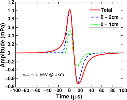
Figure 1: Simulated bipolar pressure pulse from a $10^{18}$ eV cascade at a radial distance of 1 km. Figure adapted from [14].

The cascades extend over a length of a few metres with a radius of only a few cm. In radial direction, i.e. perpendicular to the shower axis, the coherent superposition of the emitted sound waves leads to the propagation of the sound within a flat disk (often referred to as pancake) with a small opening angle. Assuming a linear dependence on the energy, the pressure pulse amplitude scales as

$$p(\mathrm{1\,km})\approx\frac{E_{casc}}{1\,\mathrm{EeV}}\,\mathrm{mPa}$$ (2)

with the energy spectral density peaking around 10 kHz.

The simulation (Fig. 1) shows that roughly half of the pressure pulse is produced within a radius of 1 cm (dot-pointed line) of the cascade, whereas the energy distribution within a radius of 2 cm (broken line) is nearly completely responsible for the final signal shape (solid line).

1.3 Acoustic Detection

Two major advantages over an optical neutrino telescope make acoustic detection worth studying. First, the attenuation length is approximately one order of magnitude higher for acoustic signals of cascades than for the Cherenkov light (order of 1 km to order of 100 m) when comparing the relevant frequency bands of the emissions. The second advantage is the much simpler sensor design and readout electronics required for acoustic measurements: No high voltage is required in the case of acoustic measurements and time scales are in the $\upmu$s range for acoustics as compared to the ns range for optics. This allows for online implementation of advanced signal processing techniques. Efficient data filters are essential, as the signal amplitude is relatively small compared to the acoustic background in the sea, which complicates the unambiguous determination of the signal.

Intensive studies are currently performed at various places to explore the potential of the acoustic detection technique. In a recent survey [15], an overview of these experimental acoustic activities is given; for the remainder of this paper, the acoustic detection system in ANTARES (AMADEUS) will be discussed.

2 The Acoustic Detection System of ANTARES (AMADEUS)

2.1 Goals

It is the declared main goal of the AMADEUS project to perform a feasibility study for a potential future large scale acoustic detector. To this end, the following aims will be pursued:

• Long term background investigations (rate of neutrino-like signals, localisation of sources);

• Investigation of signal correlations on different length scales;

• Development and tests of filter and reconstruction algorithms;

• Tests of different hydrophones and sensing methods;

• Studies of hybrid detection methods.

These goals were driving the design of the AMADEUS system, which will now be discussed.

2.2 AMADEUS as Part of ANTARES

AMADEUS is a part of the ANTARES neutrino telescope [16] in the Mediterranean Sea, which was completed on May 30th, 2008. A sketch of the complete detector is shown in Fig. 2. ANTARES is located offshore, about 40 km south of Toulon on the French coast, at a depth of about 2500 m. It comprises 12 vertical structures, the detection lines (or lines for short) plus a 13th line, called Instrumentation Line or IL07, which is equipped with instruments for monitoring the environment. Each detection line holds 25 storeys that are arranged at equal distances of 14.5 m along the line, interlinked by electro-mechanical-optical cables. A standard storey consists of a titanium support structure, holding three Optical Modules, i.e. photomultiplier tubes (PMTs) inside water tight spheres, and one Local Control Module (LCM). The LCM holds the offshore electronics and the power supply within a cylindrical titanium container (cf. Sec. 2.5). Each line is fixed on the sea floor by an anchor (called Bottom String Socket, BSS) and held vertically by a buoy.

Acoustic sensing was integrated in form of Acoustic Storeys which are modified versions of standard ANTARES storeys, replacing the PMTs by hydrophones and using custom-designed electronics for the digitisation and preprocessing of the analogue signals. Details will be discussed in the following subsections.

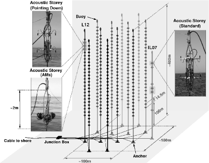
Figure 2: A sketch of the ANTARES detector. The six Acoustic Storeys are highlighted and their three different setups are shown. The setups will be described in Sec. 2.4.

The three Acoustic Storeys on the IL07 started data taking when the connection to shore of the IL07 was established on Dec. 5th, 2007, the Acoustic Storeys on Line 12 (L12) were connected to shore during the completion of ANTARES in May 2008. AMADEUS is now fully functional with 34 of its 36 sensors working.

2.3 Description of the System

It has been a fundamental design principle of the AMADEUS system to make use of standard ANTARES hard- and software as much as possible in order to minimise the effort for design and engineering and to reduce the failure risks for both ANTARES and AMADEUS by keeping the need for additional quality assurance and control measures to a minimum. In order to integrate the system successfully into the ANTARES detector, design efforts in three basic areas was necessary: First, the development of hydrophones that replace the PMTs of standard ANTARES storeys; second, the development of an offshore Acoustic ADC and preprocessing board; third, the development of on- and offline software. These subjects will be discussed in more detail in Sections 2.4, 2.6, and 2.7, respectively.

The final system has full detection capabilities (such as time synchronisation and a continuously operating data acquisition) and is scalable to a larger number of Acoustic Storeys. It combines local clusters of acoustic sensors with large cluster spacings, allowing for fast direction reconstruction with individual storeys that then can be combined to reconstruct the position of a source.

Each Acoustic Storey is equipped with six acoustic sensors with interspacings on the order of 1 m. The Acoustic Storeys 2, 3, and 6 on the IL07 are located at 180 m, 195 m, and 305 m above the sea floor, respectively. Line 12 is anchored at a horizontal distance of about 240 m from the IL07, with the Acoustic Storeys positioned at a heights of 380 m, 395 m, and 410 m. With this setup, the maximum distance between two Acoustic Storeys is 340 m. Two of the six Acoustic Storeys are shown in Fig. 3.

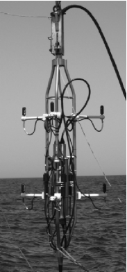
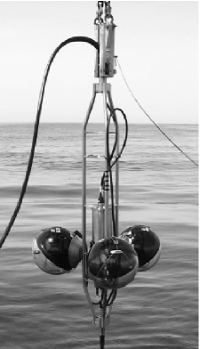
Figure 3: Storey 3 of the IL07 (left) and Storey 21 of L12 (right) during their deployment.

2.4 The Acoustic Sensors

Two types of acoustic sensors are used in AMADEUS: hydrophones and so-called Acoustic Modules (AMs, cf. Fig. 3). In both cases, the sensors are based on piezo-electrical ceramics that convert pressure waves into voltage signals, which are then amplified for readout [17]. The ceramics and amplifiers are coated in polymer plastics in the case of the hydrophones. For the AMs they are glued to the inside of the same spheres used for the Optical Modules of ANTARES. The latter non-conventional design was inspired by the idea to investigate an option for acoustic sensing that can be combined with a PMT in the same housing.

In order to obtain a complete and uniform 2$\pi$-coverage of the azimuthal angle $\phi$, the 6 sensors are distributed over the 3 AMs of the storey within a plane perpendicular to the longitudinal axis of a storey at angles of 60^∘ in $\phi$.

The three Acoustic Storeys on the IL07 house hydrophones only, whereas Storey 21 (counting from the bottom) of Line 12 holds AMs (cf. Fig. 2). In Storey 22 of Line 12, the hydrophones were mounted with their cable junction, where the sensitivity is largely reduced, pointing upwards. This allows for investigations of the directionality of background from ambient noise, which is expected to come mainly from the sea surface.

Three of the five storeys holding hydrophones are equipped with commercial hydrophones and the other two with hydrophones developed and produced at the Erlangen Centre for Astroparticle Physics (ECAP).

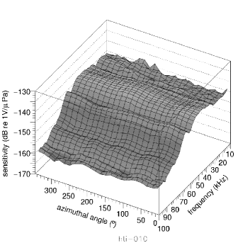
Figure 4: Sensitivity of a typical AMADEUS hydrophone as a function of frequency and azimuthal angle.

All acoustic sensors are tuned to be sensitive over the whole frequency range of interest from 1 to 50 kHz with a typical sensitivity around $-145$ dB re. 1V/$\upmu$Pa (including preamplifier) and to have a low noise level [18]. The sensitivity of a typical hydrophone is shown in Fig. 4 as a function of frequency and the azimuthal angle [19]. For a given frequency, the distribution is essentially flat on a 3 dB level.

2.5 Offshore Electronics and Acoustic Data Acquisition

In the ANTARES DAQ scheme [20], the digitisation is conducted within the offshore electronics container (LCM, cf. Sec. 2.2) on each storey by several custom-designed electronics boards, which send all digitised data to shore where data reduction is performed and the data is searched for events of interest. With its capability of timing resolutions on a nanosecond-scale and transmission of several MByte per second and per storey, it is perfectly suited for the acquisition of acoustic data. In addition, in each LCM a Compass board measures the tilt and the orientation of the storey by measuring the three components of the Earth’s magnetic field.

For the digitisation and preprocessing of the acoustic signals and for feeding them into the ANTARES data stream, the so-called AcouADC-board was designed. Each board processes the differential signals from two acoustic sensors, which results in a total of three such boards per storey.

Figure 5 shows the fully equipped LCM of an Acoustic Storey. From the left to the right, the following boards are installed: The Compass board; 3 AcouADC boards; a Data Acquisition (DAQ) board that sends the data to shore; and a Clock board that provides the timing signals to correlate measurements performed in different storeys.

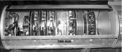
Figure 5: An LCM equipped with AcouADC-boards before insertion into its titanium housing. Visible on the left from the inside of the container are two of the three connectors which on the outside are connected to two acoustic sensors each. The boards are described in the text.

2.6 The AcouADC-Board

The AcouADC-board is shown in Fig. 6. It consists of an analogue and a digital part. The analogue part amplifies the voltage signals coming from the acoustic sensors by adjustable factors between 1 and 562 and filters the resulting signal. To protect the analogue part from potential electromagnetic interference, it is shielded by metal covers. The system has low noise and is designed to be – together with the sensors – sensitive to the acoustic background of the deep sea over a wide frequency-range. The dynamic range achieved is from the order of 1 mPa to the order of 10 Pa in RMS over the frequency range from 1 to 100 kHz.

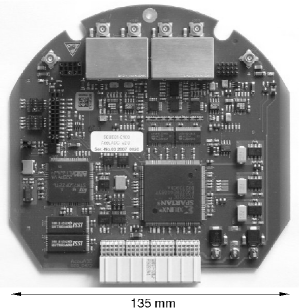
Figure 6: An AcouADC board.

The analogue filter suppresses frequencies below approx. 4 kHz and above approx. 130 kHz. The high-pass part cuts into the trailing edge of the low frequency noise of the deep-sea acoustic background [21] and thus protects the system from saturation. The low-pass part efficiently suppresses frequencies above the Nyquist frequency of 250 kHz for the sampling rate of 500 kSamples per second (kSPS). Within the passband, the filter response is essentially flat with a linear phase response.

Every individual component of the complete data taking chain was calibrated in the laboratory prior to deployment. With the deduced transfer function of the system it is possible to reconstruct the acoustic signal from the recorded one with high precision within the sensitive frequency range of the setup.

The digital part of the AcouADC-board digitises and processes the acoustic data. It is designed to be highly flexible by employing a micro controller ($\upmu$C) and a field programmable gate array (FPGA) as data processor. The $\upmu$C can be controlled with the onshore control software and is used to adjust settings of the analogue part and the data processing. Furthermore, the $\upmu$C can be used to update the firmware of the FPGA in situ.

The digitisation is done by two 16-bit ADCs for the two input channels. The digitised data from the two channels is read out in parallel by the FPGA and further processed for transmission to the DAQ board. The DAQ board then handles the transmission of the data to the onshore data processing servers.

In standard mode, the digitised data is down-sampled to 250 kSPS by the FPGA, corresponding to a downsampling by a factor of 2. Hence the frequency spectrum of interest from 1 to 100 kHz is fully contained in the data.

Onshore a dedicated computer cluster is used to process and store the acoustic data arriving from the storeys and to control the offshore DAQ. This is discussed below.

2.7 Onshore Data Processing

AMADEUS follows the same “all data to shore” strategy as ANTARES; the offshore data arrives via the TCP/IP protocol at a Gigabit switch in the ANTARES control room, where the acoustic data is separated from the standard ANTARES data and routed to the acoustic computer cluster.

The cluster currently consists of four servers of which two are used for data filtering. The filtering has the task of reducing the raw data rate of about 1.6 TB/day to about  10 GB/day for storage. Currently, three filter schemes are implemented [22]: A minimum bias trigger which records 10 s of continuous data every 30 min; a threshold trigger; a cross correlation trigger, which searches for the expected bipolar signal of a neutrino. The filtering requires coincidences of several hydrophones on each storey and can be extended to require coincidences between storeys on the same line. All parameters can be freely adjusted. The concept of local clusters (i.e. the Acoustic Storeys) has proven very efficient for fast (online) processing. Furthermore, all components are scalable which makes the system extremely flexible. Additional servers can be added or the existing ones can be replaced by the latest models if more sophisticated filter algorithms are to be implemented. In principle it is also possible to move parts of the filter into the FPGA of the AcouADC board, thereby implementing an offshore trigger which reduces the size of the data stream sent to shore.

Just like ANTARES, AMADEUS can be controlled via the Internet from essentially any place in the world and is currently operated from Erlangen. Data are centrally stored and are available remotely as well.

2.8 First Results

2.8.1 Noise Measurements

The ambient noise level in the frequency range from about 200 Hz to 50 kHz in the deep sea is assumed to be mainly determined by the agitation of the sea surface, i.e. by waves, spray and precipitation [23]. To verify these assumptions, the correlation between the weather and the RMS of the ambient noise recorded by AMADEUS was investigated. Weather data at the Hyères airport at the French coast, about 30 km north of the ANTARES site, is continuously logged by the AMADEUS onshore software. New data is made available every hour.

An upgrade of the study performed in [12] is shown in Fig. 7. Each point in the figure represents the RMS noise of a 10 s sample of data, calculated by integrating the power spectral density (PSD) in the frequency range from 1 to 50 kHz. The correlation between the wind speed and the hydrophone noise is found to be about 80%.

The results are consistent with those reported for other deep-sea sites in  [24, 25].

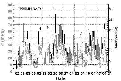
Figure 7: RMS noise recorded by a characteristic hydrophone (light dots) and windspeed (dark solid line) as a function of time, showing the correlation between the two quantities.

2.8.2 Positioning of Acoustic Storeys

A further important measurement with the AMADEUS system is the accurate determination of the relative positions of the Acoustic Storeys within the ANTARES detector (positioning). The ANTARES positioning system [26] uses transceivers (so-called pingers) at the BSS (cf. Sec. 2.2) of each line in combination with 5 acoustic receivers (positioning hydrophones) arranged along each detection line. The pingers emit tone bursts at 9 well-defined frequencies between 44 522 Hz and 60 235 Hz which can be used by AMADEUS to determine the positions of the Acoustic Storeys.

With 6 hydrophones, a complete reconstruction (position and three angles) of each Acoustic Storey can be done using the pinger signals. This is not only an interesting task on its own, but is in fact important for an accurate positioning of unknown sources as will be described below. The presence of the Compass boards (cf. Sec.2.5) allows for cross checks of the results.

Figure 8 shows the signal emitted from one pinger as recorded by two sensors in the AMs of Storey 21 and by two hydrophones of Storey 22 of Line 12. One can clearly observe the different arrival times of the signal (corresponding to different travel times of the sound from the pinger) between the storeys. For the two exemplary sensors of one storey, the smaller differences in arrival times are also clearly visible.

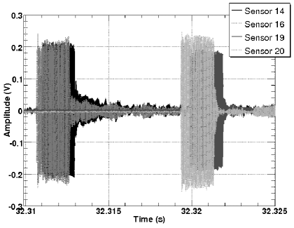
Figure 8: Pinger signals received by sensors 19, 20 (hydrophones in Storey 22 of Line 12), and sensors 14, 16 (sensors of AMs in Storey 21 of Line 12). The sensors in the lower Storey 21 receive the signal earlier than those in Storey 22. Hydrophone 20 is positioned in the bottom row, hydrophone 19 in the top row of the storey (cf. Fig. 3, left). Sensors 14 and 16 are located in different AMs, separated by about 120^∘ in $\phi$ (cf. Fig. 3, right).

Work on two methods for the positioning is currently in progress: First, the differences between the absolute time of signal emission and reception from several pingers are used to reconstruct the position of each hydrophone individually. Second, only the differences in arrival times of a pinger signal in the 6 hydrophones of a storey are used to reconstruct the direction of a pinger signal. Then the reconstructed directions are matched with the pinger pattern on the sea floor. The second method employs the same algorithms used for position reconstruction of unknown sources; this will be described now.

2.8.3 Position Reconstruction of Sources

Position reconstruction of point sources will be done by first reconstructing their direction from individual storeys and then combining the reconstructed directions from three or more storeys.

To find the direction of point sources, a beam forming algorithm is used [27]. It is designed to reconstruct plane waves, which for the geometry of a storey is a reasonable assumption for sources with distances $\gtrsim 100\,m$.

The top plot of Fig. 9 shows an exemplary signal as recorded by the topmost Acoustic Storey of the IL07. Sensors 6 and 7, 8 and 9, 10 and 11, respectively, are attached to the same rod of the storey (cf. Fig. 3); hydrophones with even numbers are located at the bottom. Signals arrive at the hydrophones positioned at the same rod almost at the same time, indicating that the direction of the source is close to horizontal.

The bottom plot shows the result of the beam forming algorithm. The intensity at a given solid angle corresponds to the probability that the source is located in that direction. Bands of increased intensity come from potential source directions where the signals from only two or three hydrophones coincide.

The most probable direction, at $\theta\approx 5^{\circ}$ and $\phi\approx-50^{\circ}$ is consistent with the intuitive interpretation of the top plot.

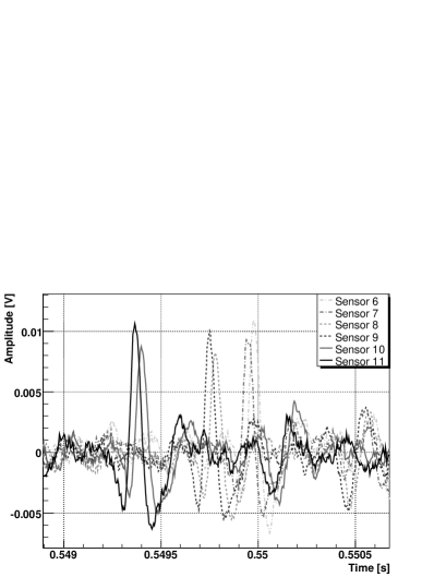
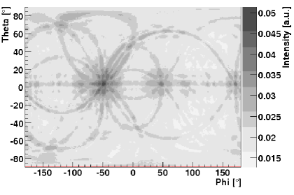
Figure 9: Reconstruction of the direction of an exemplary source. Top: Signals recorded with the hydrophones of the topmost storey of the IL07; Bottom: Result of the beamforming algorithm.

3 Conclusions and Outlook

The AMADEUS system, which is dedicated to the investigation of acoustic neutrino detection techniques, has been successfully installed in the ANTARES detector. Except for its small size, the system has all features required for an acoustic neutrino telescope and hence is excellently suited for a feasibility study of a potential future large scale acoustic neutrino telescope.

AMADEUS can be used as a multi purpose device for studies of neutrino detection techniques, position reconstruction, and marine research; for the latter, which was not discussed in this paper, discussions with external partners with expertise in the field are ongoing.

First results were presented which demonstrate the potential of AMADEUS. In particular, the Acoustic Modules allow for acoustic measurements without additional mechanical structures which might be an option for KM3NeT.

4 Acknowledgements

This study was supported by the German government through BMBF grant 05CN5WE1/7. The author wishes to thank the organizers of the VLVnT08 for a most interesting and well organised workshop.

References

- [1] IceCube Coll., A. Silvestri et al., Mod. Phys. Lett. A22 (2007) 1769.
-
[2]
KM3NeT homepage,
http://www.km3net.org. - [3] K. Greisen, Phys. Rev. Lett. 16 (1966) 748.
- [4] G.T. Zatsepin and V.A. Kuz’min, JETP Lett. 4 (1966) 78; Ž. Èksp. Teor. Fiz., (1966) 114.
- [5] Auger Coll., A. Watson et al.., Nucl. Instr. Meth. A 588 (2008) 221.
- [6] G.A. Askariyan, Sov. J. At. En. 3 (1957) 921.
- [7] G.A. Askariyan, B.A. Dolgoshein et al., Nucl. Instr. Meth. 164 (1979) 267.
- [8] J.G. Learned, Phys. Rev. 19, (1979) 3293.
- [9] L. Sulak, T. Armstrong et al., Nucl. Instr. Meth. 161 (1979) 203.
- [10] L.D. Landau and E.M. Lifshitz, Course of Theoretical Physics, Vol. 6: Fluid Mechanics, Pergamon Press, Oxford, 1959.
- [11] V. Niess and V. Bertin, Astropart. Phys. 26 (2006) 243.
- [12] K. Graf, Ph.D. Thesis, Univ. Erlangen-Nürnberg, FAU-PI1-DISS-08-001, 2008.
- [13] K. Graf, Diploma Thesis, Univ. Erlangen-Nürnberg, FAU-PI1-DIPL-04-002, 2004.
- [14] Acorne Coll., S. Bevan et al., preprint arXiv:astro-ph/0704.1025v1, 2007.
- [15] L. Thompson, Nucl. Instr. Meth. A 588 (2008) 155.
- [16] ANTARES Coll., E. Aslanides et al., preprint arXiv:astro-ph/9907432, 1999.
- [17] G. Anton et al., Astropart. Phys. 26 (2006) 301.
- [18] C. Naumann et al., Proc. of the Int. Workshop (ARENA 2005), World Scientific Publishing, Singapore (2006) 92; preprint: arXiv:astro-ph/0511243.
- [19] C. Naumann, Ph.D. Thesis, Univ. Erlangen-Nürnberg, FAU-PI4-DISS-07-002, 2007.
- [20] ANTARES Coll., J.A. Aguilar et al., Nucl. Inst. Meth. A 570(1) (2007) 107.
- [21] R.J. Urick, Principles of Underwater Sound, Peninsula Publishing, Los Altos, USA, 1983.
- [22] M. Neff, Diploma Thesis, Univ. Erlangen-Nürnberg, FAU-PI1-DIPL-07-003, 2007.
- [23] R.J. Urick, Ambient Noise in the Sea, Peninsula Publishing, Los Altos, USA, 1986.
- [24] O. Kurahashi and G. Gratta, Submitted to J Acoust. Soc. Am.; preprint arXiv:astro-ph/0712.1833v1.
- [25] NEMO Coll., submitted to Deep Sea Research I; preprint arXiv:astro-ph/0804.2913.
- [26] M. Ardid, Nucl. Instr. Meth. A, these proceedings.
- [27] C. Richardt, Diploma Thesis, Univ. Erlangen-Nürnberg, FAU-PI4-DIPL-06-001, 2006.