Abstract: Perpendicular electron dynamics and the associated collisions are discussed in relation to the collisional drift wave instability. In addition, the limit of small parallel wave numbers of this instability is studied and it is shown to yield a reduced wave frequency. It is also shown that in this case the growth rate in fact decreases for smaller parallel wave numbers, instead of growing proportional to $1/k_{z}^{2}$. As a result, the growth rate appears to be angle dependent and to reach a maximum for some specific direction of propagation. The explanation for this strange behavior is given. A similar analysis is performed for acoustic perturbations in plasmas with unmagnetized ions and magnetized electrons, in the presence of a density gradient.

PACS Numbers: 52.35.Kt, 52.30.Ex, 52.20.Fs, 52.35.Fp

I.     INTRODUCTION AND MODEL

Typically, collisions in plasmas are responsible for the damping of plasma modes. However, this does not hold for the drift wave which grows in the presence of electron collisions. The growth appears because, in the presence of collisions, the perturbed wave potential lags behind the perturbed density. This, together with the free energy stored in the density gradient, makes the mode growing. In the case when the ions are not magnetized (e.g., perturbations with frequencies above the ion gyrofrequency $\Omega_{i}$, or/and when the ion collision frequency is above $\Omega_{i}$), the ion motion will be of the sound-type, while the motion of electrons can still be described within the drift wave limits. Hence, acoustic-type perturbations in such a case may also become unstable due to the same reasons,^1,2 with the instability taking place provided that the acoustic wave frequency is below the electron diamagnetic frequency $\omega_{*e}=v_{*e}k_{y}$, $v_{*e}=-(v_{{\scriptscriptstyle T}e}^{2}/\Omega_{e})\vec{e}_{z}\times\nabla n_{0}/n_{0}$, $v_{{\scriptscriptstyle T}e}^{2}=\kappa T_{e}/m_{e}$. Physically, the instability is due to the fact that collisions prevent the electrons from moving freely and from shielding the electrostatic perturbations that involve the ion component.

In most cases, these electron collision effects are included from the electron parallel momentum.^3-6 This is because of the small inertia, which results in a dominant electron motion in the parallel direction, as compared to the perpendicular gyromotion-type dynamics. Yet, a clear distinction about when such a model is justified is rarely seen in the literature. In our recent work⁷ it is shown that the model can be used provided that

$$k_{z}^{2}\Omega_{e}^{2}/(k_{y}^{2}\nu_{e}^{2})\gg 1.$$ (1)

Here, $k_{z}$ and $k_{y}$ are the wave number components in the direction parallel and perpendicular to the direction of the magnetic field vector $\vec{B}_{0}=B_{0}\vec{e}_{z}$, respectively, and $\Omega_{e}$ denotes the electron gyrofrequency. The electron collision frequency $\nu_{e}$ may include collisions with both ions and neutrals. Numerous parameters contribute to the condition (1), and consequently it may not always be satisfied, so that in some cases it may become necessary to include collisions in the perpendicular electron dynamics as well. An obvious consequence of these collisions is that the usual drift motion of electrons (perpendicular to the force vector) will be modified, and an additional component of motion in the direction of force vector will appear as well.

In a weakly ionized plasma, the electrons may predominantly collide with neutrals. Usually, these collisions are described assuming a static and heavy neutral background so that the dynamics of the neutrals is ignored. However, the interaction between the two fluids happens due to friction, and the momentum conservation imposes that the neutral dynamics must be taken into account in spite of a big difference of mass (per unit volume) of the two fluids. In a recent study⁶ the differences between the two models are discussed in detail.

In the present work, we consistently take the dynamics of the target particles (neutrals in the present case) into account, and we discuss the domain in which the condition (1) is not satisfied.

In the case when the temperature of the heavy plasma constituents (ions and neutrals) is much below the electron temperature, we omit their thermal effects. The electron momentum equation is

$$m_{e}n_{e}\left[\frac{\partial\vec{v}_{e}}{\partial t}+(\vec{v}_{e}\cdot\nabla)\vec{v}_{e}\right]=en_{e}\nabla\phi-en_{e}\vec{v}_{e}\times\vec{B}-\kappa T_{e}\nabla n_{e}-m_{e}n_{e}\nu_{en}(\vec{v}_{e}-\vec{v}_{n}),$$ (2)

and for the neutrals we use

$$\left[\frac{\partial}{\partial t}+(\vec{v}_{n}\cdot\nabla)\right]\vec{v}_{n}=-\nu_{ne}(\vec{v}_{n}-\vec{v}_{e}).$$ (3)

The momentum conservation implies that $\nu_{ne}=m_{e}n_{e}\nu_{en}/(m_{n}n_{n})$.

II.     ON THE EQUILIBRIUM

It is seen that, assuming a stationary equilibrium and also $(\vec{v}_{n0}\cdot\nabla)\vec{v}_{n0}=0$, $(\vec{v}_{e0}\cdot\nabla)\vec{v}_{e0}=0$, from (3) we have $\vec{v}_{n0}=\vec{v}_{e0}$. At the same time, Eq. (2) yields $\vec{v}_{e0}=\vec{v}_{*e}$. Hence, due to friction both fluids move together. In most cases under laboratory conditions such a state is not expected to take place because of the long time that is needed to reach it. In order to get a better feeling about the necessary time scales, we may set a constant velocity for the electrons $\vec{v}_{e0}$ (assuming that the parameters determining the velocity are controlled externally). Using Eq. (3) we then obtain the neutral velocity: $v_{n0}/v_{e0}=1-\exp(-\nu_{ne}t)$. Now, setting for example $n_{e0}=10^{16}$ m^-3, and assuming a hydrogen plasma in hydrogen gas with $n_{n0}=10^{19}$ m^-3, $T_{e}=1$ eV, we have $\nu_{en}=1.09\cdot 10^{6}$ Hz, $\nu_{ne}=0.6$ Hz, and we find that $v_{n0}/v_{e0}\simeq 1$ within about 8 s. Here $\nu_{en}=\sigma_{en}n_{n0}v_{{\scriptscriptstyle T}e}$, and⁸ $\sigma_{en}(T_{e})\simeq 2.6\cdot 10^{-19}$ m².

Similarly, setting $n_{e0}=10^{17}$ m^-3, $n_{n0}=10^{19}$ m^-3, $T_{e}=5$ eV, we have $\nu_{en}=1.07\cdot 10^{6}$ Hz, $\nu_{ne}=5.8$ Hz, and $v_{n0}/v_{e0}\simeq 1$ within about 0.8 s. Here⁸ $\sigma_{en}(T_{e})\simeq 1.14\cdot 10^{-19}$ m².

Numbers used here are for demonstration only. Yet, similar parameters may be seen in various studies dealing with collisional drift-waves, like in the experimental work from Ref. 9 (with $T_{e}=2$ eV, $T_{i}\leq 0.1$ eV, $n_{e0}=10^{16}$ m^-3 and $\nu_{en}=2\cdot 10^{6}$ Hz). A similar density ($n_{e0}=7\cdot 10^{16}$ m^-3) but a 5 times lower electron temperature is used in the experiment in Ref. 10, while in the experiment in Ref. 11 the density and the temperature are also of the same order as in our examples, i.e., $n_{e0}=5\cdot 10^{15}$ m^-3, $T_{e}\simeq 1$ eV. In another experiment¹² the parameters are $n_{e0}=2\cdot 10^{15}$ m^-3, $T_{e}=2$ eV.

Although parameters may have very different values in various experiments, the number used in the examples above are frequently seen in the laboratory plasmas. Although the ionization degree in the two examples given above is not so small, the electron-neutral collisions are larger than electron-ion collisions. For the given parameters, the two cases yield (in kHz) $\nu_{ei}\simeq 304,\,305<\nu_{en}$, respectively. Here $\nu_{ei}$ remains almost the same because both the density and the temperature are increased. We used^13,14 the expression for the collision frequency between any two charged species $b$ and $a$

$$\nu_{ba}=4\left(\frac{2\pi}{m_{b}}\right)^{1/2}\left(\frac{q_{a}q_{b}}{4\pi\varepsilon_{0}}\right)^{2}\frac{n_{a}L_{ba}}{3(T_{b}+T_{a}m_{b}/m_{a})^{3/2}}.$$ (4)

Here, $L_{ba}=\log(\lambda_{d}/b_{0})$ is the Coulomb logarithm, $\lambda_{d}=\lambda_{db}\lambda_{da}/(\lambda_{db}^{2}+\lambda_{da}^{2})^{1/2}$ is the plasma Debye radius, and $b_{0}=[|q_{b}q_{a}|/[12\pi\varepsilon_{0}\kappa(T_{b}+T_{a})]$ is the impact parameter for Coulomb collisions.

Hence, it is correct to say that in most cases we have a ‘time evolving background plasma’. Yet, this time dependence is negligible as long as the period of the perturbations is much shorter than the equilibrium evolution time (that is of the order of $1/\nu_{ne}$). In fact, this is not a rough approximation bearing in mind the other plasma parameters and the corresponding evolution. For example, the assumed equilibrium density gradient is also time dependent because of the electron collisions, and those take place on much shorter time scales. In other words, fast electron collisions will tend to destroy the density gradient, and this may happen on short time scales, unless the density gradient is somehow kept externally (examples of that kind can be found in Refs. 15, 16). This can be seen by taking the second set of the above given parameters and assuming $B_{0}=0.01$ T, and the plasma density gradient length as $L_{n}\equiv[(dn_{e0}/dx)/n_{e0}]^{-1}=0.1$ m. The perpendicular electron diffusion velocity is then given by $D_{e}/L_{n}=3$ m/s, where $D_{e}=\nu_{en}v_{{\scriptscriptstyle T}e}^{2}/\Omega_{e}^{2}$. Hence, electron diffusion perpendicular to the magnetic field vector will tend to destroy the given density gradient in about 0.03 s and all this is entirely due to collisions. Regarding the neutrals, we stress that there may also be a continuous diffusion of neutrals from nearby regions, and those new particles have no time to be accelerated by friction within the assumed short wave period. As a result, in most cases one may perform a wave analysis neglecting the equilibrium movement of the neutrals.

III.     DERIVATIONS AND RESULTS

A. Drift wave

From Eq. (2), in the limit when the wave phase velocity and the perturbed electron velocity are much below the electron thermal velocity (equivalent to the usual massless electron approximation in the literature), we obtain the electron perpendicular velocity

$$v_{e\bot}=\frac{1}{1+\nu_{en}^{2}\alpha^{2}/\Omega_{e}^{2}}\left[\frac{1}{B_{0}}\vec{e}_{z}\times\nabla_{\bot}\phi+\frac{\nu_{en}\alpha}{\Omega_{e}}\frac{\nabla_{\bot}\phi}{B_{0}}-\frac{v_{\scriptscriptstyle{T}e}^{2}\nu_{en}\alpha}{\Omega_{e}^{2}}\frac{\nabla_{\bot}n_{e}}{n_{e}}-\frac{v_{\scriptscriptstyle{T}e}^{2}}{\Omega_{e}}\vec{e}_{z}\times\frac{\nabla_{\bot}n_{e}}{n_{e}}\right].$$ (5)

Here, $\alpha=\omega/(\omega+i\nu_{ne})$. In view of the previous discussion on equilibrium, the perturbed neutral velocity used here is $\vec{v}_{n}=i\nu_{ne}\vec{v}_{e}/(\omega+i\nu_{ne})$. The electron parallel momentum yields the parallel velocity

$$v_{ez1}=\frac{ik_{z}v_{{\scriptscriptstyle T}e}^{2}}{\nu_{en}}\frac{\omega^{2}+\nu_{ne}^{2}}{\omega^{2}-i\nu_{ne}\omega}\left(\frac{e\phi_{1}}{\kappa T_{e}}-\frac{n_{e1}}{n_{e0}}\right).$$ (6)

Using Eqs. (5, 6), and neglecting $|\nu_{en}^{2}\alpha^{2}/\Omega_{e}^{2}|$ in comparison to 1 in the denominator in Eq. (5) (the limit of magnetized electrons), from the electron continuity equation

$$\frac{\partial n_{e1}}{\partial t}+\nabla_{\bot}(n_{e}\vec{v}_{\bot e})+\nabla_{z}(n_{e0}\vec{v}_{ez1})=0,$$

we obtain

$$\frac{n_{e1}}{n_{e0}}=\frac{\omega_{*e}+iD_{p}+iD_{z}(\omega^{2}+\nu_{ne}^{2})/(\omega^{2}-i\nu_{ne}\omega)}{\omega+iD_{p}+iD_{z}(\omega^{2}+\nu_{ne}^{2})/(\omega^{2}-i\nu_{ne}\omega)}\frac{e\phi_{1}}{\kappa T_{e}}.$$ (7)

Here

$$D_{p}=\nu_{en}\alpha k_{y}^{2}\rho_{e}^{2},\quad D_{z}=k_{z}^{2}v_{{\scriptscriptstyle T}e}^{2}/\nu_{en},\quad\rho_{e}=v_{{\scriptscriptstyle T}e}/\Omega_{e}.$$

The term $D_{p}$ describes the effects of electron collisions in the perpendicular direction. Note that neglecting the neutral dynamics here is equivalent to setting $\nu_{ne}=0$, yielding $\alpha=1$, and this corresponds to the model in Refs. 1, 2. In the case $D_{p}=0$, Eq. (7) becomes the same as the corresponding equation from Ref. 6. It is seen also that the assumption $|D_{z}/D_{p}|\gg 1$ yields the condition (1). In the present work we are interested in the domain when this limit is either reversed or the ratio is of order of 1.

For cold collisionless ions we use the same model as in Ref. 6, i.e., the ions are only subject to the electromagnetic force, so that the momentum equation for magnetized ions is

$$m_{i}n_{i}\left[\frac{\partial\vec{v}_{i}}{\partial t}+(\vec{v}_{i}\cdot\nabla)\vec{v}_{i}\right]=-en_{i}\nabla\phi+en_{i}\vec{v}_{i}\times\vec{B}.$$ (8)

Using this, from the ion continuity we obtain

$$\frac{n_{i1}}{n_{i0}}=\left(\frac{\omega_{*e}}{\omega}+\frac{k_{z}^{2}c_{s}^{2}}{\omega^{2}}-k_{y}^{2}\rho_{s}^{2}\right)\,\frac{e\phi_{1}}{\kappa T_{e}},\quad\rho_{s}=c_{s}/\Omega_{i},\quad c_{s}^{2}=\kappa T_{e}/m_{i}.$$ (9)

The dispersion equation within the quasi-neutrality limit reads

$$\frac{\omega_{*e}}{\omega}+\frac{k_{z}^{2}c_{s}^{2}}{\omega^{2}}-k_{y}^{2}\rho_{s}^{2}=\frac{\omega_{*e}+iD_{p}+iD_{z}(\omega^{2}+\nu_{ne}^{2})/(\omega^{2}-i\nu_{ne}\omega)}{\omega+iD_{p}+iD_{z}(\omega^{2}+\nu_{ne}^{2})/(\omega^{2}-i\nu_{ne}\omega)}.$$ (10)

The term with the sound speed is due to the ion parallel response and it is known to introduce the threshold for the instability.⁶

For negligible collisions, the right-hand side in Eq. (10) reduces to 1, and we have the simple expression for the drift wave in an ideal plasma

$$\omega^{2}(1+k_{y}^{2}\rho_{s}^{2})-\omega_{*e}\omega-k_{z}^{2}c_{s}^{2}=0.$$ (11)

It has two solutions, one positive coupled drift-acoustic mode, and one negative acoustic mode.

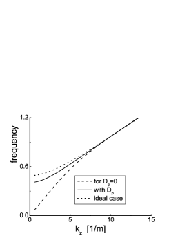
Figure 1: The positive solutions of Eq. (10) without (dashed line) and with (full line) the perpendicular electron collisions included. Dotted line is the positive solution of Eq. (11). Frequency is normalized to $\omega_{*e}$.

The full Eq. (10) is solved numerically for several values of the neutral density. In Fig. 1 the frequency (normalized to $\omega_{*e}$) of the positive drift-acoustic solution is given in terms of the parallel wave-number $k_{z}$, for a fixed $k_{y}=10^{3}$ 1/m, and for $n_{n0}=10^{21}$ m^-3, $n_{e0}=5\cdot 10^{16}$ m^-3, $T_{e}=11600$ K, $B_{0}=0.1$ T, and $L_{n}=0.1$ m. This particular set of parameters can easily be achieved in laboratory conditions, and it is taken in order to have perfectly satisfied all conditions used in the model. This is seen from the following. $\omega_{*e}\simeq 10^{5}$ Hz, and the mode frequency is below $\omega_{*e}$ or of the same order, so that for the given parameters both electrons and ions are magnetized, $\Omega_{i}\simeq 10^{7}$ Hz, $\Omega_{e}=2\cdot 10^{10}$ Hz. The electron collision frequency with ions $\nu_{ei}$ is about 3 orders of magnitude below $\nu_{en}\simeq 10^{8}$ Hz, and it is therefore negligible. The plasma $\beta$ is about $10^{-6}$ and the electrostatic limit is justified. Large $k_{y}$ implies a reasonably well satisfied local analysis condition because $L_{n}/\lambda_{y}\simeq 16$. In the range of frequencies and $k_{z}$ given in Fig. 1, the ratio $(\omega/k_{z})/v_{{\scriptscriptstyle T}e}$ changes between 0.12 (for $k_{z}=1$) and 0.02 (for $k_{z}=14$), so that neglecting the left-hand side of the electron momentum equation is justified. Observe also that the electron mean free path is $v_{{\scriptscriptstyle T}e}/\nu_{en}\simeq 0.004$ m, while the shortest parallel wavelength is about 0.45 m, so the condition for the fluid model for electrons is well satisfied.

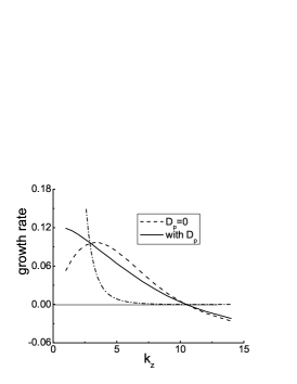
Figure 2: Growth rate (normalized to $\omega_{*e}$) associated with the mode from Fig. 1. The dash-dot line refers to the growth rate which follows from Eq. (12), i.e., in the limits $D_{p}=0$ and $|\omega|\ll D_{z}$).

The dotted line in Fig. 1 is the solution which follows from the ideal case (11) (i.e., for the right-hand side in Eq. (10) equal to unity). In the limit of small $k_{z}$ this solution goes to $0.49\,\omega_{*e}$ because here $k_{y}\rho_{s}=1.02$. The dashed line is the numerical solution of Eq. (10) in the case when the electron collisions in the perpendicular direction are simply ignored ($D_{p}=0$). The full line is the solution including $D_{p}$. Observe the significant difference in the limit of small $k_{z}$ between the ideal mode frequency and the collisional modes. The effect of keeping $D_{p}$ here is practically to restore (at least quantitatively) the drift-like behavior of the mode.

The growth-rates associated with the frequency from Fig. 1 are presented in Fig. 2, showing an angle dependence and having a maximum at $k_{z}$ around $3$ (for the case $D_{p}=0$). We note that a similar angle dependence (though due to ion collisions) was obtained recently in the problem of current driven acoustic modes.^7,17 In the present case, the origin of the maximum, and of the reduced frequency for small $k_{z}$ is different and can be understood from the following. If $D_{p}$ is completely omitted, the approximative growth rate is given by⁶

$$\omega_{i}\simeq\frac{\omega_{r}^{2}}{D_{z}}\frac{\omega_{r}^{2}k_{y}^{2}\rho_{s}^{2}-k_{z}^{2}c_{s}^{2}}{\omega_{r}^{2}(1+k_{y}^{2}\rho_{s}^{2})+k_{z}^{2}c_{s}^{2}}.$$ (12)

Here $\omega_{r,i}$ denote the real and imaginary parts of the frequency, respectively. This analytic expression is obtained and valid within the approximation

$$|\omega_{r}|\ll D_{z}.$$ (13)

Hence, in this limit, the growth rate appears to be proportional to $1/D_{z}\sim 1/k_{z}^{2}$ and it strongly grows for small $k_{z}$. This is presented by the dash-dotted line in Fig. 2.

The condition (13) can be written as

$$\frac{|\omega_{r}|/k_{z}}{v_{{\scriptscriptstyle T}e}}\ll\frac{k_{z}v_{{\scriptscriptstyle T}e}}{\nu_{en}}.$$ (14)

The right-hand side is the ratio of the mean free path and the parallel wavelength, and it must be below 1 to have a proper fluid theory. The left-hand side (the ratio of the parallel wave phase speed and the electron thermal speed) must also be below 1 within the model used here (neglected left-hand side of the electron momentum equation). However, although both sides separately have some physical meaning and both are below 1, their mutual ratio is arbitrary and, therefore, the conditions (13,14) do not have to be satisfied. In fact, in our present case, for the parameters used above and in the limit of small $k_{z}$, the frequency $|\omega_{r}|$ becomes of the order of $D_{z}$ or even larger. This reverses the direction of the dash-dotted line in Fig. 2 for small enough $k_{z}$, and we obtain the dashed line (the case $D_{p}=0$). Hence, for small $k_{z}$ the growth rate takes a completely different shape if the condition (1) is satisfied, and if the dispersion equation is solved for parameters when the condition (13) does not hold.

Remark that the condition (13) is usually used for analytical convenience. We have shown here that this excludes an important limit in which the growth rate may be drastically reduced.

In addition to this, in the limit opposite to the condition (1), the perpendicular electron dynamics and perpendicular collisions must be taken into account. As a result the growth rate is additionally modified and it is given by the full line in Fig. 2. This effect appears because for $k_{z}<6$ 1/m, we have $D_{p}>D_{z}$ as seen from Fig. 3, where $D_{p}$ is presented normalized to local values of $D_{z}(k_{z})$. Basically the same reasons are behind the reduced frequency in Fig. 1.

Figure 3: $D_{p}=\nu_{en}k_{y}^{2}\rho_{e}^{2}$ normalized to $D_{z}$ in terms of $k_{z}$ corresponding to Figs. 1, 2.

Note also that the growth rate in Fig. 2 becomes negative around $k_{z}\simeq 10.45$ 1/m. The reason for this may be seen from Eq. (12), where the growth rate changes the sign if $k_{z}^{2}>\omega_{r}^{2}k_{y}^{2}\rho_{s}^{2}/c_{s}^{2}$. This is the instability threshold mentioned earlier, due to the parallel ion response. The point of the sign change is almost the same for all three cases from Fig. 2 because all parameters, except the frequency, are kept constant, and the frequency itself for the three cases is almost the same (see Fig. 1).

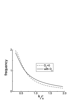
Figure 4: The normalized frequency as positive solution of Eq. (10) in terms of $k_{y}$.

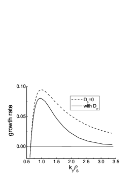
Figure 5: The normalized growth rate for the frequency from Fig. 4.

Equation (10) is solved also in terms of $k_{y}$, for a fixed $k_{z}=4$ m^-1 and for the same values for the other parameters as above. This yields $D_{z}=25810$ Hz and $\rho_{s}=10^{-3}$ m. The result for the frequency and the growth rate (both in units of $\omega_{*e}$) is presented in Figs. 4, 5. In the given range of $\vec{k}$ the ratio $D_{p}/D_{z}$ has values in the range from $0.2$ (for $k_{y}=300$ 1/m) to $15$ (for $k_{y}=2500$). The growth rate changes the sign at $k_{y}\rho_{s}\simeq 0.65$. Setting $D_{p}=0$ provides the dashed lines in Figs. 4 and 5. The growth rate is lower in the presence of $D_{p}$. Physically, in the situation with $D_{p}\neq 0$, light electrons have more possibility to shield electrostatic perturbations by moving now also in the perpendicular direction (due to the collisions). As a result, the growth rate is reduced.

B. Acoustic wave

In the case of high wave frequencies

$$\Omega_{e}\gg|\omega|\gg\Omega_{i},$$ (15)

the ions are unmagnetized and their response is the same as in an ion acoustic mode, while the electron dynamics is the same as in the previous text. The ion continuity and momentum equation (8) without the Lorentz force instead of Eq. (9) yield $n_{i1}/n_{i0}=(k^{2}c_{s}^{2}/\omega^{2})e\phi_{1}/(\kappa T_{e})$, $k^{2}=k_{y}^{2}+k_{z}^{2}$. The dispersion equation now reads

$$\frac{k^{2}c_{s}^{2}}{\omega^{2}}=\frac{\omega_{*e}+iD_{p}+iD_{z}(\omega^{2}+\nu_{ne}^{2})/(\omega^{2}-i\nu_{ne}\omega)}{\omega+iD_{p}+iD_{z}(\omega^{2}+\nu_{ne}^{2})/(\omega^{2}-i\nu_{ne}\omega)}.$$ (16)

Equation (16) is solved for modified parameters in order to have the conditions (15) satisfied. Hence, we take heavier (argon) ions $m_{i}=40m_{p}$, $m_{n}=m_{i}$, and $T_{e}=5$ eV, $n_{n0}=10^{21}$ m^-3, $n_{e0}=n_{i0}=5\cdot 10^{16}$ m^-3, $B_{0}=0.01$ T, $L_{n}=0.1$ m. For these parameters we have¹⁸ $\sigma_{en}=8.7\cdot 10^{-20}$ m². We set $k_{y}=7\cdot 10^{2}$ 1/m and solve Eq. (16) in terms of $k_{z}$. The results are given in Figs. 6 and 7. It is seen that the perpendicular electron collisions drastically destabilize the mode. In the limit of small $k_{z}$, the growth rate in Fig. 7 is about 70 times larger. Note that for $k_{z}=0.3$ 1/m we have $D_{p}/D_{z}=141$, while for $k_{z}=14$ 1/m this ratio is only 0.06.

For large $k_{z}$ values, the growth rate in Fig. 7 decreases with $k_{z}$ similar to the solutions from Ref. 2. It can also be shown that the growth rate becomes larger when $n_{n0}$ is increased (i.e., for larger collision frequency). These features are in agreement with an approximative analytical solution that may be derived from Eq. (16) assuming a dominance of the $D_{z}$ term.

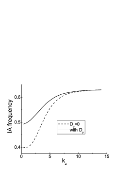
Figure 6: Ion acoustic frequency (normalized to $\omega_{*e}$) as the positive solution of Eq. (16).

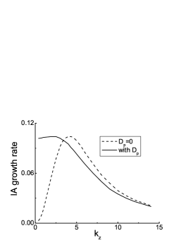
Figure 7: The normalized growth rate associated with the acoustic mode from Fig. 6.

IV.     CONCLUSIONS

To summarize, we have presented some details of the collisional drift wave instability that are usually overlooked in the literature. In particular, the mode behavior for small parallel wave numbers is usually described within the limit given by the condition (13), resulting in a strongly increasing growth rate proportional to $1/k_{z}^{2}$. We have shown that in the opposite limit the mode is considerably modified, both the frequency and the growth rate are reduced. As a result, the growth rate appears to be angle dependent, reaching a maximum value for a certain angle of propagation. Furthermore, the effect of collisions on the perpendicular electron dynamics and on the collisional drift wave instability is discussed. It is shown to have effect on both the wave frequency and the growth rate, as presented in Figs. 1, 2, 4, and 5.

Similar effects of the perpendicular electron collisions are shown for the acoustic-type mode in plasmas with magnetized electrons and unmagnetized ions. In such plasmas, the ion electrostatic perturbations result in acoustic modes regardless of the angle of propagation. The physics of the mode is described in the classic Ref. 1, and was also discussed more recently in Ref. 2.

The collision frequency has been taken constant in the present work, following standard semi-empirical models used in the literature, yet a recent study¹⁹ shows that it can be significantly modified depending on ion temperature. This is an issue that requires further investigations. In any case we believe that the results presented here should be taken into account in studies dealing with dissipative drift-type instabilities, like those in Refs. 20-23. A most obvious example where the instability conditions will clearly be modified is the recent Ref. 24 dealing with drift dissipative instability in a toroidal device.

The model and results obtained here may be used also in application to space plasmas. A most obvious example where the theory works is the lower solar atmosphere with the ionization ratio which may be as low as $10^{-6}$ (in photosphere, with typical temperatures of around $5\cdot 10^{3}$ K), and it changes with the altitude to become of the order of 1 in the chromosphere (at the altitude of about 2200 km), and grows towards corona where neutrals are absent. Some aspects of the drift waves in solar atmosphere may be found in Refs. 25, 26. A similar situation with altitude-dependent parameters suitable for the drift wave may be found in the terrestrial ionosphere.²⁷ Another interesting aspect of the application to space problems may be seen also in Ref. 28 dealing with Hall thrusters used in spacecrafts propulsion, with dominant collisions with neutrals and a geometry suitable for the drift wave analysis.

We have briefly discussed the issue of the equilibrium in such a three-component collisional plasma. One important point that follows from it, and that has been discussed briefly, is the possibility of equilibrium macroscopic flows of neutrals in a magnetized plasma. Such flows may be generated by diamagnetic drifts of plasma species in an inhomogeneous plasma. The diamagnetic drift itself is not a macroscopic plasma flow but the effect of gyromotion of plasma species in the presence of a density gradient. Yet, as such it may still generate real macroscopic flows of the neutral component of the plasma. This is due to friction and may have important implications, in particular for space plasmas. Similar effects should appear in the presence of a magnetic field gradient.

References

- [1] A. B. Mikhailovskii, Theory of Plasma Instabilities, vol. 2 (Consultants Bureau, New York, 1974) p. 192.
- [2] J. Vranjes, D. Petrovic, B. P. Pandey, and S. Poedts, Phys. Plasmas 15, 072104 (2008).
- [3] J. Weiland, Collective Modes in Inhomogeneous Plasmas (Institute of Physics Pub., Bristol, 2000) p. 32.
- [4] J. Vranjes and S. Poedts, Phys. Lett. A 348, 346 (2006).
- [5] J. Vranjes, B. P. Pandey, and S. Poedts, Planet. Space Sci. 54, 695 (2006).
- [6] J. Vranjes and S. Poedts, Phys. Plasmas 15, 034504 (2008).
- [7] J. Vranjes and S. Poedts, Phys. Plasmas 13, 122103 (2006).
- [8] B. Bedersen and L. J. Kiefer, Rev. Mod. Phys. 43, 601 (1971).
- [9] E. Marden Marshall, R. F. Ellis, and J. E. Walsh, Plasma Phys. Contr. Fusion 28, 1461 (1986).
- [10] R. E. Rowberg and A. Y. Wong, Phys. Fluids 13, 661 (1970).
- [11] C. L. Xaplanteris, Astrophys. Space. Sci. 139, 233 (1987).
- [12] E. Gravier, X. Caron, G. Bonhomme, T. Pierre, and J. L. Briançon, Eur. Phys. J. D 8, 451 (2000).
- [13] L. Spitzer, Physics of fully ionized gasses (Intersience Publishers, New York, London, 1984) p. 135.
- [14] J. Vranjes, M. Kono, S. Poedts, and M. Y. Tanaka, Phys. Plasmas 15, 092107 (2008).
- [15] K. Nagaoka, A. Okamoto, S. Yoshimura, M. Kono, and M. Y. Tanaka, Phys. Rev. Lett. 89, 075001 (2002).
- [16] M. Y. Tanaka, K. Nagaoka, A. Okamoto, S. Yoshimura, and M. Kono, IEEE Trans. Plas. Phys. 33, 454 (2005).
- [17] J. Vranjes and S. Poedts, Phys. Plasmas 13, 052103 (2006).
- [18] V. E. Fortov and I. T. Iakubov, The Physics of Non-Ideal Plasma (World Scientific, Singapore, 2000) p. 380.
- [19] L. Conde, L. F. Ibán̋ez, and J. Lambás, Phys. Rev. E. 78, 026407 (2008).
- [20] W. Horton, Rev. Mod. Phys. 71, 735 (1999).
- [21] A. Zeiler, J. F. Drake, and B. Rogers, Phys. Plasmas 4, 2134 (1997).
- [22] R. J. Hastie, J. J. Ramos, and F. Porcelli, Phys. Plasmas 10, 4405 (2003).
- [23] W. J. Boss, S. Futatani, S. Benkadda, M. Farge, and K. Schneider, Phys. Plasmas 15, 072305 (2008).
- [24] J. C. Perez, W. Horton, K. Gentle, W. L. Rowan, K. Lee, and R. B. Dahlburg, Phys. Plasmas 13, 032101 (2006).
- [25] J. Vranjes and S. Poedts, Astron. Astrophys. 458, 635 (2006).
- [26] H. Saleem, J. Vranjes, and S. Poedts, Astron. Astrophys. 471, 289 (2007).
- [27] M. C. Kelley, The Earth’s ionosphere (Acad. Press, London, 1989) pp. 148-151.
- [28] E. Y. Choueiri, Phys. Plasmas 8, 1411 (2001).