Quantum computation of multifractal exponents through the quantum wavelet transform

Abstract

We study the use of the quantum wavelet transform to extract efficiently information about the multifractal exponents for multifractal quantum states. We show that, combined with quantum simulation algorithms, it enables to build quantum algorithms for multifractal exponents with a polynomial gain compared to classical simulations. Numerical results indicate that a rough estimate of fractality could be obtained exponentially fast. Our findings are relevant e.g. for quantum simulations of multifractal quantum maps and of the Anderson model at the metal-insulator transition.

I Introduction

It has been realized over the past twenty years that the specific properties of quantum mechanics enable to conceive new ways of treating and manipulating information (for a review see e.g. nielsen ). In particular, the idea of a quantum computer has been put forth. Such a device would perform computation on quantum registers usually thought of as made of qubits. It has been shown that quantum algorithms can be devised which are asymptotically faster than classical algorithms, the most famous examples being the Shor algorithm which factorizes numbers exponentially faster than any known classical algorithm shor , and the Grover algorithm which searches a database quadratically faster than any possible classical procedure grover .

However, not so many efficient quantum algorithms have been found, and it is still unclear which problems can be treated faster on a quantum computer and how efficiently. One of the first possibilities to be put forward was the simulation of quantum systems on quantum computers, which was first envisioned by Feynman feynman and then made more precise in several subsequent works lloyd ; abrams ; schack ; georshe ; saw1 ; georlevshe ; georlev . Some of these algorithms have been experimentally implemented in few-qubit systems such as in cory . Recent more mathematical works have established more rigorously that a quantum computer can indeed simulate efficiently (i.e. exponentially fast) a wide class of quantum systems israeli ; sanders . However, these works were mostly concerned with the possibility of efficient simulation of a quantum system. To be complete and comparable with a classical algorithm, a quantum algorithm should not only perform a computation in an efficient way, but also be able to extract information from the result of this computation in an efficient way. Thus a quantum algorithm should also include specification of how information is extracted from the final wavefunction at the end of the simulation. Several proposals have been made in order to extract efficiently information from a quantum simulation, looking at the fidelity fidelity , the spectral statistics formfactor , the localization length loclength , the Wigner function georlevshe , or the diffusion constants como ; georlev . It has been found that the final gain compared to classical simulation depends on the choice of the observable and on the measurement procedure, and can dramatically change the efficiency of the quantum simulation. It is therefore important to explore in more detail which quantities can be extracted from a quantum simulation and with which efficiency.

The quantum systems studied up to now in this setting were in general localized or extended in the computational basis. However, there exists another class of quantum systems intermediate between these two types, whose wavefunctions are multifractal. Such properties appear in physical systems, for example in wavefunctions of electrons in a disordered potential at the Anderson transition between metal and insulator mirlin ; cuevas ; garciagarcia ; fyodorov , or at the quantum Hall transition huckestein . It has been shown that simple systems displaying such properties can be simulated exponentially fast on a quantum computer pomer ; interm . It is therefore interesting to assess if the multifractal properties can be extracted from the resulting wavefunction at the end of the quantum simulation, and with which efficiency.

In this paper, we explore different strategies to measure the multifractality, and more precisely multifractal exponents, from a quantum wavefunction produced by a quantum simulation, and assess their efficiency. In particular, we assess the interest of the wavelet transform to perform such tasks. This transform is a generalization of the Fourier transform using basis functions localized in both position and momentum instead of the sinusoidal waves of the Fourier transform. The wavelet transform has been used with great success in data treatment and data compression, and has been included in compression standards such as MPEG4. It has been shown that a quantum wavelet transform (QWT) can be implemented efficiently on a quantum computer WT1 ; WT2 ; WT3 , but it has been seldom used in quantum algorithms, with few exceptions wavealg2 ; terraneo ; husimi ; wavealg1 ; wavealg . As concerns multifractal analysis, recent theoretical progress in classical data treatment have shown that the wavelet transform can be used as a versatile tool to explore multifractality of various phenomena, such as DNA sequences, turbulence or cloud structure arneodo .

Our results show that, although the methods of classical multifractal analysis cannot be directly implemented efficiently on a quantum computer, suitable modifications of the method combined with amplitude amplification enable to get multifractal coefficients from a wavefunction with polynomial efficiency. This translates into complete algorithms of quantum simulations including measurements which are polynomially faster than corresponding classical algorithms. We also give numerical indications that the wavelet transform may enable to assess a rough measure of the degree of fractality of a wavefunction with exponential efficiency.

II Multifractal quantum states

Multifractal quantum states are characteristic of certain systems intermediate between chaos and integrability. They have been found at the Anderson transition between metal and insulator, i.e. between extended states and localized states, and also at quantum Hall transitions mirlin ; cuevas ; garciagarcia ; fyodorov ; huckestein . More generally, they correspond to a whole class of systems whose spectral statistics, for example, are of the semi-poisson type gerland intermediate between Random Matrix statistics (associated with ergodic states) and Poisson statistics (associated with integrable or localized states).

Multifractality properties of wavefunctions are described by a whole set of generalized fractal dimensions $D_{q}$. For a vector $|\psi\rangle=\sum_{i=1}^{N}\psi_{i}|i\rangle$ in an $N$-dimensional Hilbert space, the spectrum $\tau_{q}$ is defined through the scaling of the moments

$$\sum_{i=1}^{N}|\psi_{i}|^{2q}\propto N^{-\tau_{q}}.$$ (1)

The multifractal exponents, or generalized multifractal dimensions, are related to the spectrum by the relation

$$D_{q}=\frac{\tau_{q}}{q-1}.$$ (2)

In order to investigate properties of multifractal quantum states, simple models have been devised which exhibit such properties giraud ; bogomolny ; garciagarcia . A particularly simple example is the quantization of a map on the torus which has been shown to exhibit a whole range of multifractal properties, depending on one parameter. The classical map is given by

$$\begin{array}[]{cccc}\bar{p}&=&p+\gamma&\mathrm{(mod}\;\mathrm{1)}\\ \bar{q}&=&q+2\bar{p}&\mathrm{(mod}\;\mathrm{1)}\end{array}.$$ (3)

The quantization of this map yields a unitary evolution operator acting on a Hilbert space of dimension $N=1/(2\pi\hbar)$ which can be expressed in momentum space by the $N\times N$ matrix giraud ; bogomolny

$$U_{pp^{\prime}}=\frac{e^{i\phi_{p}}}{N}\frac{1-e^{2i\pi N\gamma}}{1-e^{2i\pi(p-p^{\prime}+N\gamma)/N}},$$ (4)

with $\phi_{p}=-2\pi p^{2}/N$. From this quantized map one can construct an ensemble of random matrices, taking $\phi_{p}$ as independent random variables uniformly distributed in $[0,2\pi[$ bogomolny .

This map has different properties depending on the parameter $\gamma$. Indeed, for irrational $\gamma$, the map possesses the characteristics of systems displaying quantum chaos, with eigenstates ergodic over the phase space and spectral statistics of the eigenphases of the evolution operator following random matrix predictions. In contrast, for rational $\gamma=n_{1}/n_{2}$, the spectral statistics are of the semi-Poisson type intermediate between those of integrable and chaotic systems bogomolny . The eigenstates in momentum representation display multifractal properties studied in martin . The fractality depends on $n_{2}$ and is stronger for smaller $n_{2}$. Thus the set of quantum maps $U$ with rational $\gamma$ gives a random matrix ensemble with intermediate statistics (ISRM) whose multifractal properties are controlled by the parameter $n_{2}$. Such a map can be implemented efficiently on a quantum computer interm , as an exponentially large vector can be evolved through (4) with a polynomial number of gates. This map will be used as a benchmark for numerical simulations in this paper, since it represents a simple but non-trivial example of system with multifractal properties depending on one parameter and which can be simulated efficiently on a quantum computer.

On the other hand, this system is complicated enough to be hard to tackle analytically. In order to test the accuracy of our approach for the estimation of multifractal dimensions on a simpler system where all exponents can be analytically computed, we consider the situation where the coefficients of the quantum state are given by a multifractal cascade. Multifractal cascades are examples of multifractal measures for which generalized dimensions can be calculated analytically. The simplest example was proposed in cascade ; it is a special case of a Bernoulli measure on a two-scale Cantor set procaccia . It can be constructed by the following process: one breaks an initial interval into two equal parts, attributes a weight $p_{1}$ to one half and $p_{2}=1-p_{1}$ to the other, and repeats the process (keeping the same weights $(p_{1},p_{2})$ constant) on the newly constructed intervals. After $k$ steps, there are $2^{k}$ intervals and the weight of each interval is of the form $p_{1}^{r}p_{2}^{k-r}$ for some $r$, $0\leq r\leq k$. The generalized dimensions can be shown to be given by procaccia

$$D_{q}=\frac{1}{1-q}\log_{2}\left(p_{1}^{q}+p_{2}^{q}\right).$$ (5)

In this way one can construct quantum “cascade” states of size $2^{k}$ whose amplitudes squared are given by the weights of the cascade.

III Wavelet transforms and multifractal properties

An important procedure has been developed in recent years to extract multifractal exponents from a distribution. It uses the wavelet transform waveletbook , a generalization of the Fourier transform which expands a function on the wavelet basis instead of the Fourier basis. Contrary to the sinusoidal waves which compose the Fourier basis, which have specified frequencies but are extended in position space, the wavelets are localized both in momentum and position. They can thus probe many properties which are difficult to reach with the standard Fourier transform, such as singularities of the distribution. This has made wavelet transforms a popular tool in recent developments of e.g. image or sound treatment and compression in classical information, such as the formats JPEG and MPEG.

Wavelet transforms are based on a single function $g$, called the analyzing wavelet or mother wavelet. The wavelet transform of a function $f$ is a function $T_{f}$ of two variables defined as

$$T_{f}(a,b)=\frac{1}{a}\int dx\,f(x)g\left(\frac{x-b}{a}\right).$$ (6)

Variable $a$ corresponds to the scale at which the function $f$ is analyzed, while $b$ is a space variable. Thus $T_{f}(a,b)$ is a measure of how close the function $f$ is to the mother wavelet at point $b$ and at scale $a$.

If the function $f$ is sampled as a $N$-dimensional vector where $N=2^{n}$, the wavelet transform can be discretized and implemented as a unitary transformation, resulting in a Fast Wavelet Transform (FWT) analogous to the Fast Fourier Transform. The scale parameter $a$ takes values $1,1/2,1/4,...1/2^{n-1}$, while the space parameter $b$ varies over ${\cal L}(a)=\{1,2,\ldots,1/a\}$ at scale $a$. A discrete version of the mother wavelet is constructed recursively at each scale. Commonly used mother wavelets for the FWT include the Haar wavelet Haar and the Daubechies wavelet daub . Throughout the paper, we will use the Daubechies 4 discrete wavelet transform in the numerical simulations. It has been shown that a quantum wavelet transform (QWT) implementing such discrete wavelet transforms can be performed efficiently on a quantum computer WT1 ; WT2 ; WT3 , namely an exponentially large vector $\sum_{i=0}^{N-1}\psi_{i}|i\rangle$ of size $N=2^{n}$ can be transformed in a number of operations polynomial in $n$ into a vector $\sum_{a,b}T_{\psi}(a,b)|a,b\rangle$, where the wavelet transform at scale $a$ is stored on the computational basis vectors $|a,.\rangle$.

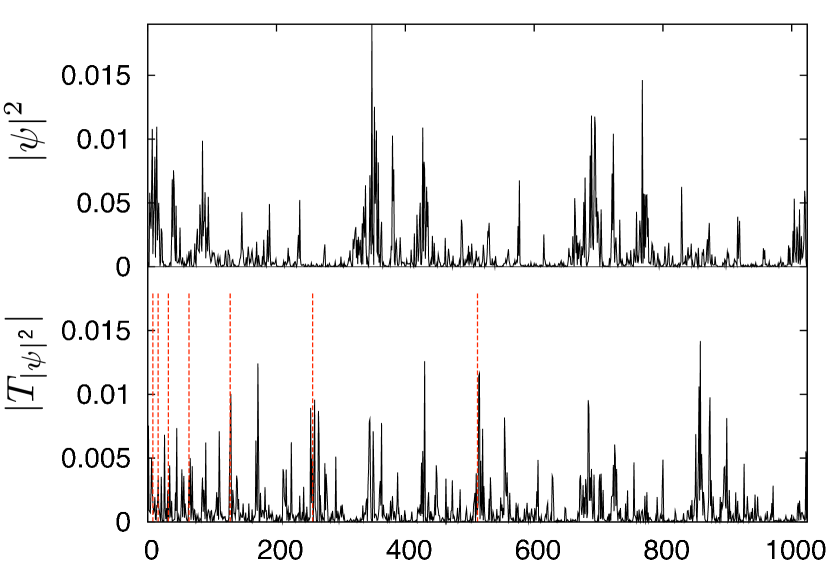
Figure 1: (Color online) Example of one eigenfunction of (4) (top) and its wavelet transform (bottom). The red/grey dashed vertical lines on the bottom panel separate the different scales in the wavelet transform.

The wavelet transform has been put forward recently as a tool for extracting the value of the exponents from a multifractal distribution. These exponents are usually quite hard to extract numerically, and are very unstable, since the values obtained depend on the chosen numerical method up to very large system sizes. An example of a multifractal distribution (for an eigenvector of (4)) is shown on Fig.1, together with its wavelet transform. One sees that the wavelet transform does not look especially simpler than the original distribution. However, recent works have shown arneodo ; arnschol ; arnbook that the wavelet transform allows to extract the exponents of the distribution $f$, using the maxima of the wavelet transform at each scale. Such methods based on the wavelet transform have enabled to extract multifractal exponents in complicated physical systems of great fundamental and technological importance such as e.g. DNA sequences arne2 , fully developed turbulence arne3 or high-resolution satellite images of cloud structure arne4 .

However, these methods use the continuous wavelet transform, which is delicate to implement for many systems of interest. A variation of the wavelet method developed in allemands ; coreens uses instead of the maxima of the continuous wavelet transform the sum of the values of the discrete wavelet transform, properly normalized at each scale. One defines the partition function

$$Z(a,q)=\sum_{b\in{\cal L}(a)}\left[\frac{|T_{f}(a,b)|}{\sum_{b\in{\cal L}(a)}|T_{f}(a,b)|}\right]^{q}$$ (7)

where $a$ is the scale and ${\cal L}(a)$ is the interval corresponding to each scale $a$. The asymptotic behavior of the partition function at small scales is governed by the generalized dimensions as

$$Z(a,q)\sim_{a\rightarrow 0^{+}}a^{\tau_{q}}$$ (8)

with $\tau_{q}\equiv D_{q}(q-1)$.

IV quantum algorithms for multifractal exponents

There does not seem to be a simple way to implement efficiently the maxima method on a quantum computer. However, as we show below, the scaling (8) of the partition function (7) can be evaluated on a quantum computer, and gives rise to quantum algorithms for estimating multifractal exponents $\tau_{q}$. Our goal in this section is to construct quantum algorithms which use Eqs. (7)-(8) in order to efficiently extract information about multifractal properties, in the situation where quantum states are obtained by quantum simulation.

IV.1 Wavelet transform of $|\psi|^{2}$

For a given state $\psi$, the weights $|\psi_{i}|^{2}/\sum_{i}|\psi_{i}|^{2}$ define a normalized measure on the unit interval. Following Eq. (7), the partition function that describes the multifractal properties of $\psi$ reads

$$Z_{|\psi|^{2}}(a,q)=\sum_{b\in{\cal L}(a)}\left[\frac{|T_{|\psi|^{2}}(a,b)|}{\sum_{b\in{\cal L}(a)}|T_{|\psi|^{2}}(a,b)|}\right]^{q},$$ (9)

where as before $a$ is the scale and ${\cal L}(a)$ is the interval corresponding to each scale $a$. The denominator in Eq. (9) is a normalization that ensures that at each scale the sum yields a proper probability measure. The multifractal exponents $\tau_{q}$ can be extracted in the limit of small scales through the scaling (8).

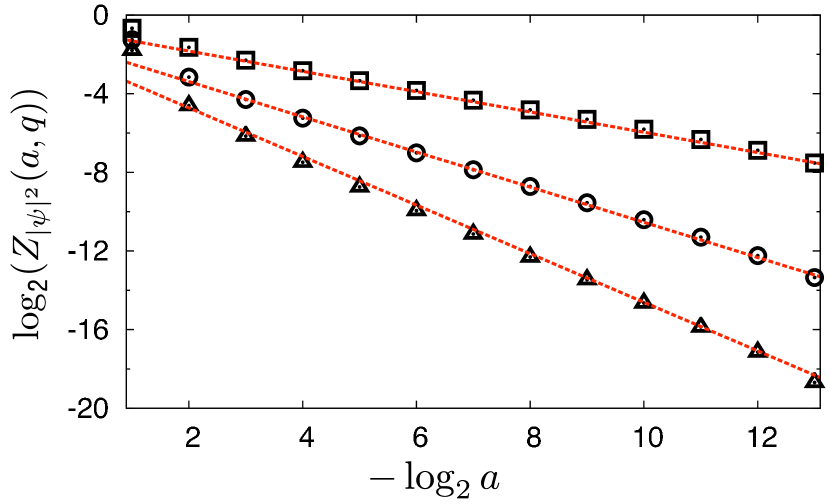
Figure 2: (Color online) Average of $\log_{2}Z_{|\psi|^{2}}(a,q)$ as a function of the scale $a$ for $q=2$ ($\square$), $q=3$ ($\circ$), $q=4$ ($\triangle$). The slope of the fitting straight lines (dashed) gives $-\tau_{q}$. Averaging is done over $\sim 25000$ eigenvectors of (4) of size $N=2^{14}$ for $n_{2}=3$ ($\gamma=1/3$).

As is shown in Fig.2 for eigenvectors of (4), the partition function (9) indeed scales as predicted for multifractal wavefunctions, and gives the multifractal exponent $\tau_{q}$, whence the fractal dimensions. For instance the linear fit for $q=2$ has a slope giving $\tau_{2}=D_{2}=0.52$, which is consistent with the fractal dimension obtained in martin .

We now show that it is possible to implement such sums on a quantum computer in the case $q=2$, allowing to obtain the multifractal exponent $\tau_{2}$ for wavefunctions produced by a quantum simulation algorithm. The first step is to adapt such a quantum simulation algorithm to our present purpose. Usually the vector $|\psi\rangle$ we are interested in comes out of the quantum simulation with its components $\psi_{i}$ as amplitudes of the basis states. However in (9) the wavelet transform is applied to a vector whose components are $|\psi_{i}|^{2}$. Thus one first has to modify the quantum simulation in order to produce $\sum_{i}|\psi_{i}|^{2}|i\rangle$ rather than $\sum_{i}\psi_{i}|i\rangle$. To do so, one should build the product of two iterates on separate registers, in order to obtain a state $\sum_{i=0}^{N-1}\sum_{j=0}^{N-1}\psi_{i}\psi^{*}_{j}|i\rangle|j\rangle$, and then use amplitude amplification to keep only the diagonal terms $i=j$. Let us detail the steps. We start with two copies of an initial state $|\psi_{0}\rangle=\sum_{i=0}^{N-1}\psi^{0}_{i}|p_{i}\rangle$ in momentum representation: $|\psi_{0}\rangle\otimes|\psi^{*}_{0}\rangle=\sum_{i=0}^{N-1}\sum_{j=0}^{N-1}\psi^{0}_{i}\psi^{0*}_{j}|p_{i}\rangle|p_{j}\rangle$. Here $\psi_{0}^{*}$ is the complex conjugate of $\psi_{0}$ and $|p_{i}\rangle$ are the basis vectors in the momentum representation. This step requires $2n$ qubits to hold the values of the wavefunction on a $N$-dimensional Hilbert space, where $N=2^{n}$. Let us consider the iterations of such a vector through a quantum map. We can apply the algorithm implementing the evolution operator of the intermediate map $\hat{U}$ as explained in interm to each subsystem independently. The operator on one subsystem can be described as the product of diagonal operators followed by Fourier transforms. On the quantum registers this corresponds to multiplication by phases followed by quantum Fourier transform (QFT). The multiplication by phases of each coefficient keeps the separability of the state into its two subsystems. The QFT mixes only states with the same value of the other register attached, and therefore also keeps the factorized form. Let us see how this works for one iteration: multiplication of the first register by the diagonal operator $e^{-i\phi_{p_{i}}}\delta_{ij}$ performs the transformation

$$\sum_{i=0}^{N-1}\sum_{j=0}^{N-1}\psi^{0}_{i}\psi^{0*}_{j}|p_{i}\rangle|p_{j}\rangle\rightarrow\sum_{i=0}^{N-1}\sum_{j=0}^{N-1}e^{-i\phi_{p_{i}}}\psi^{0}_{i}\psi^{0*}_{j}|p_{i}\rangle|p_{j}\rangle.$$ (10)

After QFT with respect to $p_{i}$ followed by multiplication by $e^{2i\pi\gamma\hat{q}}$ the state can be put under the form

$$\sum_{j=0}^{N-1}(\sum_{i=0}^{N-1}b_{i}|q_{i}\rangle)\psi^{0*}_{j}|p_{j}\rangle.$$ (11)

Under QFT with respect to $q_{i}$ we get

$$\sum_{j=0}^{N-1}(\sum_{i=0}^{N-1}\psi^{1}_{i}|p_{i}\rangle)\psi^{0*}_{j}|p_{j}\rangle = (\sum_{i=0}^{N-1}\psi^{1}_{i}|p_{i}\rangle)\otimes(\sum_{j=0}^{N-1}\psi^{0*}_{j}|p_{j}\rangle)$$ (12)

$$= \hat{U}|\psi_{0}\rangle\otimes|\psi^{*}_{0}\rangle.$$

Thus iterations can be carried independently on each register. By applying the same steps $2t$ times, we obtain the state $\hat{U}^{t}|\psi_{0}\rangle\otimes\hat{U}^{*t}|\psi^{*}_{0}\rangle=\sum_{i=0}^{N-1}\sum_{j=0}^{N-1}\psi^{t}_{i}|p_{i}\rangle\otimes\psi^{t*}_{j}|p_{j}\rangle$. This can be done in $O(tn^{2})$ gates if we use the algorithm of interm to implement $\hat{U}$. Once this is done, the state after $t$ iterations is a product of two copies of the state $|\psi\rangle$ whose fractal dimensions we are looking for. In the momentum representation it takes the form $\sum_{i,j}\psi_{i}\psi^{*}_{j}|p_{i}\rangle\otimes|p_{j}\rangle$. We wish to select in this double sum the terms with $i=j$. This can be done through amplitude amplification amplification , which is a generalization of Grover’s algorithm grover . The latter starts from an equal superposition of $N$ states, and in $\sqrt{N}$ operations brings the amplitude of a specific state close to one. Amplitude amplification increases the amplitude of a whole subspace. If $P$ is a projector onto this subspace, and $\hat{V}$ is the operator taking $|0\rangle$ to a state having a nonzero projection on the desired subspace, repeated iterations of $\hat{V}(I-2|0\rangle\langle 0|)\hat{V}^{-1}(I-2P)$ on $\hat{V}|0\rangle$ will increase the projection. Indeed, if one writes $\hat{V}|0\rangle=P\hat{V}|0\rangle+(I-P)\hat{V}|0\rangle$, the result of one iteration is to rotate the state toward $P\hat{V}|0\rangle$ staying in the subspace spanned by $P\hat{V}|0\rangle$ and $(I-P)\hat{V}|0\rangle$. If $x=|P\hat{V}|0\rangle|^{2}$, one can check that after one iteration the state is $(4x^{2}-3)P\hat{V}|0\rangle+(4x^{2}-1)(I-P)\hat{V}|0\rangle$, with a component along $(I-P)\hat{V}|0\rangle$ decreased by $4x^{2}$.

If $\hat{V}$ is chosen to be $\hat{U}^{t}\otimes\hat{U}^{*t}$ and $P$ to be a projector on the space corresponding to $i=j$, the process of amplitude amplification from the initial state $|\psi_{0}\rangle\otimes|\psi^{*}_{0}\rangle$ will bring the probability of $i=j$ to one. The number of iterations depends on the probability inside this space compared to total probability. As we want to select terms with $p_{i}=p_{j}$ the subspace we are searching for has a relative weight $\sum_{i=0}^{N-1}|\psi_{i}|^{4}$. For a fractal state this quantity scales as $N^{-\alpha}$, with $\alpha\leq 1$. Thus the total number of Grover iterations will be of the order $N^{\alpha/2}$. So in the worst case of $\alpha\approx 1$, the total cost of building the state $\sum_{i=0}^{N-1}|\psi_{i}|^{2}|p_{i}\rangle|p_{i}\rangle$ is $\sim t\sqrt{N}$. The more fractal the system is, the smaller $\alpha$ is, and the more efficient the algorithm is.

Once the state $\sum_{i=0}^{N-1}|\psi_{i}|^{2}|p_{i}\rangle|p_{i}\rangle$ is built, the second register is set back to $|0\rangle$ and the QWT can be applied at a logarithmic cost on the first register. This yields a state $\sum_{a,b}T_{|\psi|^{2}}(a,b)|a,b\rangle$. Then measurement of $a$ will give an histogram of $\sum_{b}|T_{|\Psi|^{2}}(a,b)|^{2}$ for the different values of $a$. The denominator of (9) can be obtained through classical approximations with lower resolution (e.g. half the number of qubits), and the exponent can be obtained from the slope of $\log_{2}Z_{|\psi|^{2}}(a,q)$. The total cost for applying $t$ iterations of the map and extracting the fractal dimension is thus $O(tN^{\alpha/2})$ operations, as opposed to $tN$ for the classical algorithm.

Here we considered vectors obtained by iterations of a map. It is however important to study also eigenvectors. The procedure above cannot be generalized directly, since eigenvectors are to be selected by phase estimation first before the partition function can be calculated.

In order to obtain eigenvectors of a map $U$, one first builds the state $2^{-n}\sum_{t}|t\rangle|U^{t}\psi_{0}\rangle\sum_{t}^{\prime}|t^{\prime}\rangle|U^{*t^{\prime}}\psi^{*}_{0}\rangle$ with $0\leq t\leq N-1$. The initial state $|\psi_{0}\rangle$ should be simple enough to be built efficiently (for example $|00...0\rangle$). To obtain the double sum one starts from $2^{-n}\sum_{t}|t\rangle|\psi_{0}\rangle\sum_{t}^{\prime}|t^{\prime}\rangle|\psi^{*}_{0}\rangle$, easy to obtain from $|0\rangle|\psi_{0}\rangle|0\rangle|\psi^{*}_{0}\rangle$ by Hadamard gates. Then one applies $U$ or $U^{*}$ in the same way as above on each register $t$ or $t^{\prime}$ times, by using conditional gates, in a manner similar to the one explained in trace . We then do the QFT on both registers $|t\rangle$ and $|t^{\prime}\rangle$, giving $2^{-n}\sum_{\theta}a_{\theta}|\theta\rangle|\psi_{\theta}\rangle\sum_{\theta^{\prime}}a_{\theta^{\prime}}|-\theta^{\prime}\rangle|\psi^{*}_{\theta^{\prime}}\rangle$, where $\theta$ are the eigenphases of the unitary quantum map. This corresponds to performing two phase estimations in parallel on each copy of $|\psi\rangle$. The functions $a_{\theta}$ are peaked around the eigenvalues of $U$, with $|\psi_{\theta}\rangle$ the corresponding eigenvector. Then we use amplitude amplification to select the same eigenvalue $\theta=-\theta^{\prime}$. This costs in general at most $N\sqrt{N}$ operations in total. It is possible to improve this bound by taking advantage of the fact that the wavefunction is multifractal, as was the case for iterations. For example in the simulation of (4), the wavefunction is multifractal in the $p$ representation. So if one starts with a basis vector in $p$ representation, the eigenvectors will have a multifractal distribution on this particular basis vector. Thus selecting $\theta=-\theta^{\prime}$ costs a factor $N^{\alpha/2}$. The selection of the diagonal part of the product of the two same eigenvectors costs another $N^{\alpha/2}$. This implies that the total cost to get the same eigenvalue will be $N^{1+\alpha}$, as opposed to $N^{2}$ for the classical algorithm.

Then the wavelet transform can be applied at a logarithmic cost. This yields the numerator of the formula (9) in $N^{1+\alpha}$ operations. The denominator can be obtained through classical approximations with lower resolution, giving a total cost of $N^{1+\alpha}$ as opposed to $N^{2}$ for the classical algorithm, but with the approximation that the denominator corresponds to a lower resolution. Then measurement of $a$ will give an histogram of $\sum_{b}|T_{|\Psi|^{2}}(a,b)|^{2}$ for the different values of $a$, from which the exponent can be extracted.

The method described here enables to obtain the numerator in (9) more efficiently on a quantum computer than on a classical device. Nevertheless, this procedure needs to use a low-resolution approximation of the denominator in (9) which will be obtained on a classical device. We have made numerical experiments to see if computing classically the denominator with twice less qubits (thus keeping the polynomial gain for the whole procedure) leads to a good approximation of the $\tau_{q}$. However, we were not able to reach a large enough number of qubits to have sensible data with half the qubits, and thus the evidence was inconclusive (data not shown), although we believe the procedure should give a better approximation to $\tau_{q}$ than with a computation of both numerator and denominators at low resolution. To circumvent this problem, it is worthwile to investigate if a modification of the partition function (9) would be more adapted to quantum computation.

IV.2 Wavelet transform of $\psi$

In the preceding algorithm, one had to approximate the denominator in (9) through low resolution classical computation. This entails an approximation of the multifractal exponent which can be difficult to control. In order to circumvent this difficulty, we studied the accuracy of a different formula for the partition function which is more efficient to implement on a quantum computer. This is a generalization of the partition function (9) which involves the wavelet transform of $\psi$ instead of $|\psi|^{2}$, namely

$$Z_{\psi}(a,q)=\sum_{b\in{\cal L}(a)}\left[\frac{|T_{\psi}(a,b)|^{2}}{\sum_{b\in{\cal L}(a)}|T_{\psi}(a,b)|^{2}}\right]^{q}.$$ (13)

The advantage of such a choice for the partition function is that the QWT can now be performed directly on a state $\sum_{i=0}^{N-1}\psi_{i}|i\rangle$, without using amplitude amplification to build the $|\psi_{i}|^{2}$ on the registers. This new partition function $Z_{\psi}$ actually also has a scaling $a^{\tau_{q}}$ for $a\rightarrow 0$ as in (8), as illustrated by Fig.3.

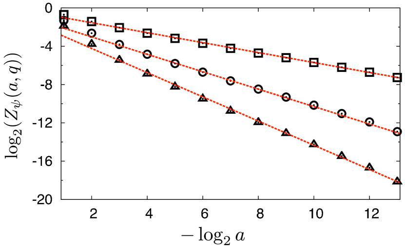
Figure 3: (Color online) Average of $\log_{2}Z_{\psi}(a,q)$ as a function of the scale $a$ for $q=2$ ($\square$), $q=3$ ($\circ$), $q=4$ ($\triangle$). The slope of the fitting straight lines (dashed) gives $-\tau_{q}$. Averaging is done over $\sim 25000$ eigenvectors of (4) of size $N=2^{14}$ for $n_{2}=3$ ($\gamma=1/3$).

In fact, the quantities $\sum_{b\in{\cal L}(a)}|T_{\psi}(a,b)|^{2q}$ appearing in the numerator of Eq. (13) should themselves contain some information about fractality of the state $\psi$. Let us denote $\tau_{q}^{\prime}$ the corresponding multifractal exponents, that is the exponents extracted from the partition function (13) without the normalization, that is from the scaling

$$\sum_{b\in{\cal L}(a)}|T_{\psi}(a,b)|^{2q}\sim a^{\tau^{\prime}_{q}}.$$ (14)

It might seem at first sight that the computation of $\tau^{\prime}_{1}$ through QWT could yield an exponential gain over classical computation, provided exponentially fast quantum simulation of the state is possible. Indeed, for iterations of simple vectors (such as basis vectors) by an efficiently simulable quantum map such as (4), the whole process of iterations of the map and QWT is exponentially fast, and the asymptotic behaviour of $\sum_{b\in{\cal L}(a)}|T_{\psi}(a,b)|^{2}$ can be estimated also exponentially fast by measuring $a$ and making an histogram of the probabilities to extract the exponent $\tau^{\prime}_{1}$. For the multifractal cascade, the slopes seem to converge to a precise value which depends on the fractality (see Fig.4). However, our numerical data show that for the quantum map (4) the asymptotic behaviour of $\sum_{b\in{\cal L}(a)}|T_{\psi}(a,b)|^{2}$ is independent of the system and seems universal. This can be seen in Fig.5, where the multifractal exponents $\tau^{\prime}_{q}$ extracted from $\sum_{b\in{\cal L}(a)}|T_{\psi}(a,b)|^{2q}$ are shown. It therefore seems that $\sum_{b\in{\cal L}(a)}|T_{\psi}(a,b)|^{2}$, which can be obtained exponentially fast, does not yield useful information in the case corresponding to actual quantum simulation. We shall return to this quantity in Subsection C.

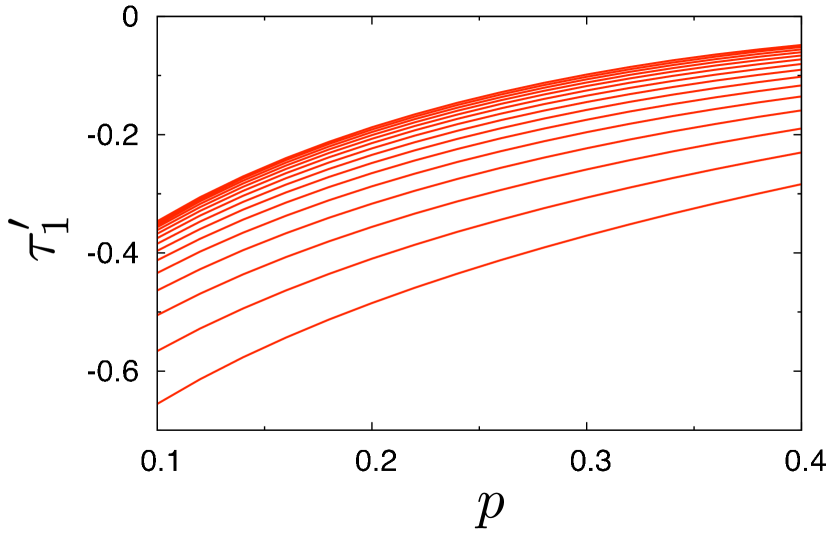
Figure 4: (Color online) $\tau^{\prime}_{1}$ as a function of $p$ for the multifractal cascade; vectors have size $N=2^{n}$ with $n$ varying from top to bottom from $n=6$ to $n=20$.

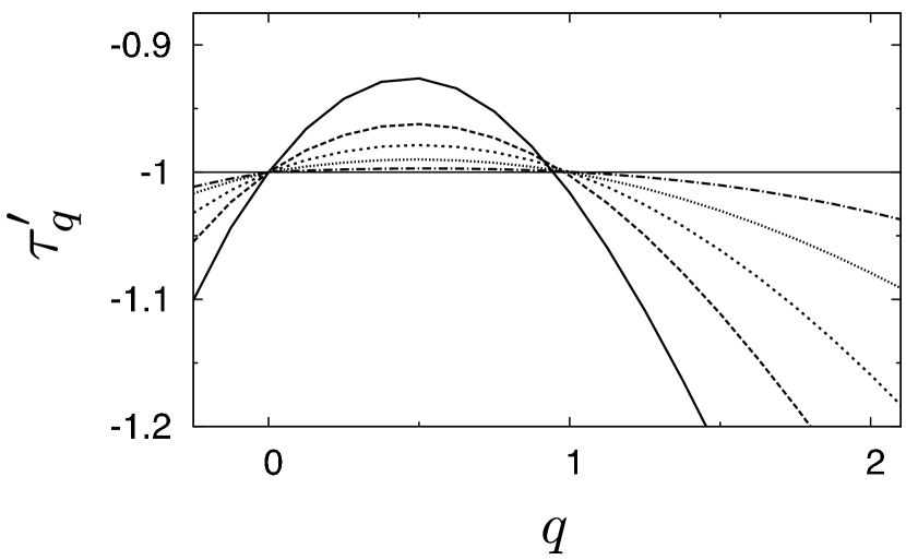
Figure 5: $\tau^{\prime}_{q}$ for eigenvectors of (4) as a function of $q$ for $n_{2}=3$ (solid), $n_{2}=5$ (dashed), $n_{2}=7$ (dotted), $n_{2}=11$ (small-dot), and $n_{2}=13$ (dash-dot) ($n_{1}=1$). Average is done over $\sim 25000$ eigenvectors of size $2^{12}$.

In the remaining part of this subsection, we study the quantum simulation of the quantity $Z_{\psi}(a,q)$, again for $q=2$. We show that it can be obtained with polynomial gain over classical computation. Since the denominator of (13) is obtained exponentially fast, being just $\sum_{b\in{\cal L}(a)}|T_{\psi}(a,b)|^{2}$, the exponent $\tau_{2}$ is now obtained without resorting to approximations.

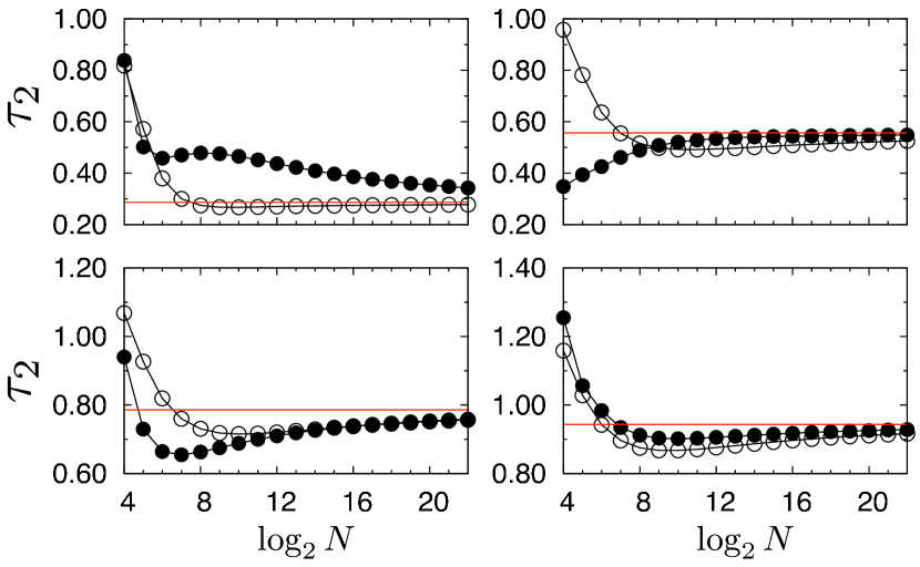
Figure 6: (Color online) $\tau_{2}$ for the multifractal cascade computed with $Z_{|\psi|^{2}}(a,q)$ (9) (filled circles) and $Z_{\psi}(a,q)$ (13)(empty circles). The values of $p$ are from left to right and top to bottom, $p=0.1,0.2,0.3,0.4$. The straight horizontal lines are the theoretical values $\tau_{2}=-\log_{2}(p^{2}+(1-p)^{2})$.

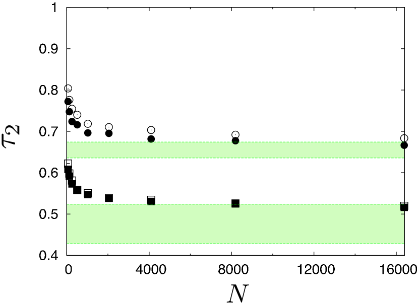
Figure 7: (Color online) $\tau_{2}$ for eigenvectors of the intermediate map (4) computed with $Z_{|\psi|^{2}}(a,q)$ (9) (filled symbols) and $Z_{\psi}(a,q)$ (13) (empty symbols) for $n_{2}=3$ (squares) and $n_{2}=5$ (circles) ($n_{1}=1$). Average is done over $\sim 25\,000$ eigenvectors. The green/grey area shows the corresponding range of values obtained in martin (top $n_{2}=5$, down $n_{2}=3$).

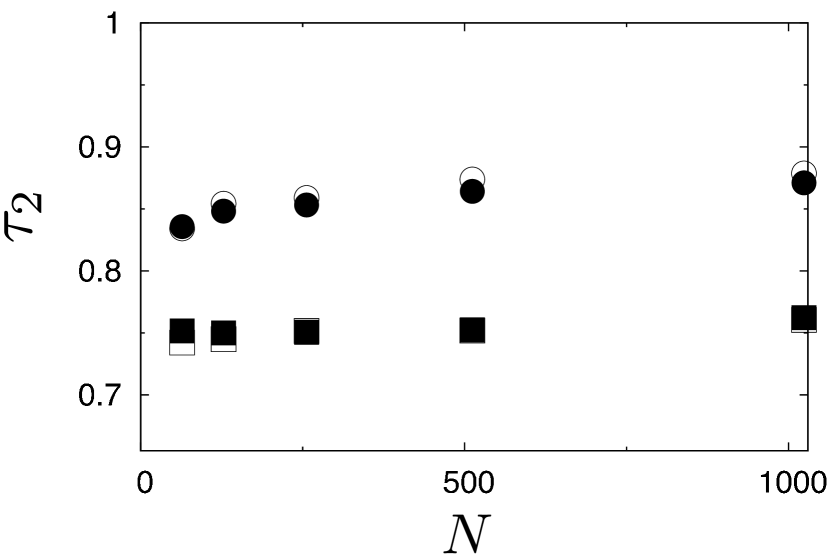
Figure 8: $\tau_{2}$ for iterates of column vectors corresponding to time $t=1000$ of the intermediate map (4) computed with $Z_{|\psi|^{2}}(a,q)$ (9) (filled symbols) and $Z_{\psi}(a,q)$ (13) (empty symbols) for $n_{2}=3$ (squares) and $n_{2}=5$ (circles) ($n_{1}=1$). The number of vectors averaged for each case is $\sim 25\,000$.

Figs.6,7,8 show the behaviour of the numerical $\tau_{2}$ obtained from (13) for increasing system sizes, plotted together with the one obtained from (9). One sees that both converge to the same value for large system size. In the case of the multifractal cascade (Fig.6), they both converge to the analytical value given by Eq. (5), while for eigenvectors of the intermediate quantum map (4) (Fig.7) the asymptotic value is within the uncertainty of the different numerical methods used in martin . For iterates of column vectors of (4) (Fig.8), one also obtains similar results with both methods. This seems to indicate that this new partition function gives asymptotically the same result as (9), and can be used reliably to obtain this multifractal exponent.

To get the quantities $\sum_{b\in{\cal L}(a)}|T_{\psi}(a,b)|^{4}$, the numerator of (13) for $Z_{\psi}(a,2)$, one needs to build the state $\sum_{a,b}|T_{\psi}(a,b)|^{2}|a,b\rangle$. This can be done through a procedure similar to the one exposed in Subsection A. One starts from two iterations of the map, followed by two QWT. This yields the state

$$\sum_{a,b}T_{\psi}(a,b)|a,b\rangle\sum_{a^{\prime},b^{\prime}}T_{\psi}(a^{\prime},b^{\prime})|a^{\prime},b^{\prime}\rangle.$$

Then amplitude amplification can be used to select the part $a=a^{\prime}$ and $b=b^{\prime}$ in this expression, leading in at most $\sqrt{N}$ operations to the state $\sum_{a,b}|T_{\psi}(a,b)|^{2}|a,b\rangle$. From this state, measurement of register $|a\rangle$ yields a value of $a$ with probability $\sum_{b\in{\cal L}(a)}|T_{\psi}(a,b)|^{4}$; an histogram of these probabilities thus yields the exponent. In the case of the iterations of vectors through a quantum map such as (4), the total cost of the method is at most of order $t\sqrt{N}$ operations, to be compared to $tN$ for iterating the vector classically up to time $t$. Actually the scaling of the second moment of the wavelet transform vector $T_{\psi}$ has an exponent $\beta$ smaller than 1 which means that $T_{\psi}$ is also fractal. This gives an actual quantum cost of $tN^{\beta/2}$, where $\beta<1$ for fractal wavelet transform.

For eigenvectors of a quantum map, the same reasoning as above leads to a quantum algorithm costing of the order $N^{1+\alpha/2+\beta/2}$ operations, as opposed to $N^{2}$ for the classical algorithm, where $\alpha<1$ for fractal wavefunctions and $\beta<1$ for fractal wavelet transform.

IV.3 Possibility of exponential gain

We have seen at the beginning of Subsection B that $\sum_{b\in{\cal L}(a)}|T_{\psi}(a,b)|^{2}$ can be estimated exponentially fast on a quantum computer. The corresponding exponent gave useful information for the cascade (see Fig.4), but in the case of the quantum map (4), our simulations showed that the numerically extracted exponent converges for large system size to the same value, whatever the fractality of the system (see Fig.5). Nevertheless, we present numerical data on Fig.9 showing that for the multifractal quantum map (4), although all exponents converge to the same value, the rate of convergence seems to depend on the fractality of the system. If these numerical indications correspond to a generic phenomenon for multifractal quantum systems, then a rough estimate of the degree of fractality of the system could be obtained exponentially fast compared to classical algorithms.

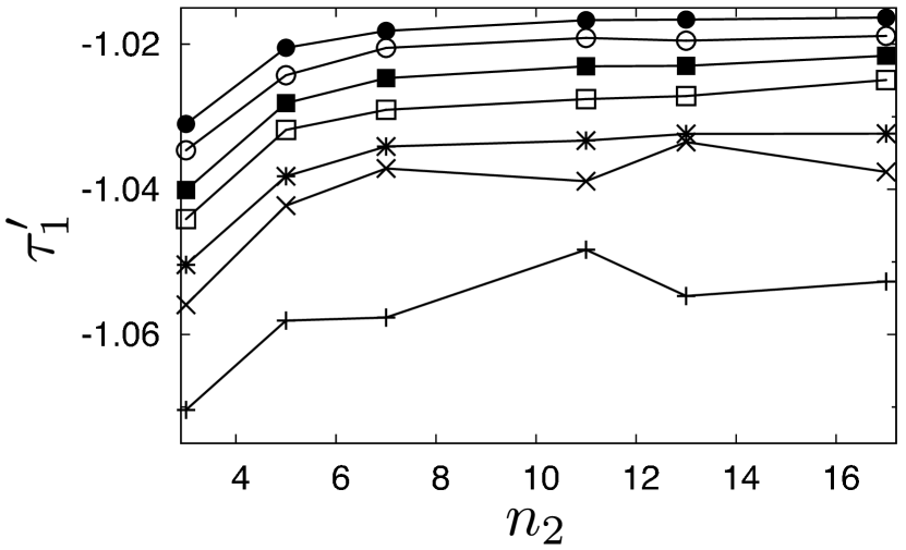
Figure 9: $\tau^{\prime}_{1}=\sum_{b}|T_{\psi}|^{2}$ for eigenvectors of the intermediate map (4) as a function of $n_{2}$ (with $n_{1}=1$) for different values of $n$ (number of qubits) bottom to top $n=6,7,8,9,10,11,12$. The number of vectors averaged for each case is $\sim 25\,000$.

V conclusion

In this paper we have investigated the use of the quantum wavelet transform to extract information (namely the multifractal exponents) from a quantum wavefunction produced by an efficient quantum simulation on a quantum computer. We have shown that various partition functions which can be extracted from a wavefunction indeed enable to obtain the multifractal exponents. Unfortunately, the partition function which can be obtained exponentially fast does not yield useful results, although our numerical results indicate that it can give exponentially fast a rough idea of the degree of fractality in a system. We have shown that other partition functions can be extracted, with a polynomial gain compared to classical computation.

Our results indicate that the quantum wavelet transform can be applied efficiently to extract useful information for certain types of quantum simulation. They show that once the full process of simulation and measurement is taken into account, quantum simulations of multifractal quantum systems yield polynomially efficient quantum algorithms, which may be exponential in certain cases. Our results also show that the quantum wavelet transform is an effective tool which acts in a complementary way from the more usual quantum Fourier transform, enabling to extract certain types of information efficiently.

We thank Marcello Terraneo and John Martin for helpful discussions, CalMiP for access to their supercomputers, and the French ANR (project INFOSYSQQ) and the IST-FET program of the EC (project EUROSQIP) for funding.

References

- (1) M. A. Nielsen and I. L. Chuang, Quantum computation and quantum information, Cambridge Univ. Press, 2000.
- (2) P. W. Shor, in Proc. 35th Annu. Symp. Foundations of Computer Science (ed. Goldwasser, S. ), 124 (IEEE Computer Society, Los Alamitos, CA, 1994).
- (3) L. K. Grover, Phys. Rev. Lett. 79, 325 (1997).
- (4) R. P. Feynman, Found. Phys. 16, 507 (1986).
- (5) S. Lloyd, Science 273, 1073 (1996).
- (6) D. S. Abrams and S. Lloyd, Phys. Rev. Lett. 79, 2586 (1997).
- (7) R. Schack, Phys. Rev. A 57, 1634 (1998).
- (8) B. Georgeot and D. L. Shepelyansky, Phys. Rev. Lett. 86, 2890 (2001).
- (9) G. Benenti, G. Casati, S. Montangero and D. L. Shepelyansky, Phys. Rev. Lett. 87, 227901 (2001).
- (10) B. Lévi, B. Georgeot and D. L. Shepelyansky, Phys. Rev. E 67, 046220 (2003).
- (11) B. Lévi and B. Georgeot, Phys. Rev. E 70, 056218 (2004).
- (12) M. K. Henry, J. Emerson, R. Martinez and D. G. Cory Phys. Rev. A 74, 062317 (2006).
- (13) D. Aharonov and A. Ta-Shma, in Proc. 35th Annual ACM Symp. on Theory of Computing, 20 (2003).
- (14) D. W. Berry, G. Ahokas, R. Cleve and B. C. Sanders, Comm. Math. Phys. 270(2), 359 (2007).
- (15) J. Emerson, Y. S. Weinstein, S. Lloyd and D. G. Cory, Phys. Rev. Lett. 89, 284102 (2002).
- (16) D. Poulin, R. Laflamme, G. J. Milburn and J. P. Paz, Phys. Rev. A 68, 022302 (2003).
- (17) G. Benenti, G. Casati, S. Montangero and D. L. Shepelyansky, Phys. Rev. A 67, 052312 (2003).
- (18) G. Benenti, G. Casati and S. Montangero, Quant. Inf. Proc. 3, 273 (2004).
- (19) F. Evers and A. D. Mirlin, Phys. Rev. Lett. 84, 3690 (2000); A. D. Mirlin, Phys. Rep. 326, 259 (2000).
- (20) E. Cuevas, M. Ortuno, V. Gasparian and A. Perez-Garrido, Phys. Rev. Lett. 88, 016401 (2001).
- (21) A. M. Garcia-Garcia and J. Wang, Phys. Rev. Lett. 94, 244102 (2005).
- (22) A. D. Mirlin, Y. V. Fyodorov, A. Mildenberger and F. Evers, Phys. Rev. Lett. 97, 046803 (2006).
- (23) B. Huckestein, Rev. Mod. Phys. 67, 357 (1995).
- (24) A. A. Pomeransky and D. L. Shepelyansky, Phys. Rev. A 69, 014302 (2004).
- (25) O. Giraud and B. Georgeot, Phys. Rev. A 72, 042312 (2005).
- (26) P. Høyer, preprint quant-ph/9702028.
- (27) A. Fijaney and C. Williams, Lecture Notes in Computer Science 1509, 10 (Springer, 1998) and preprint quant-ph/9809004.
- (28) A. Klappenecker, in Wavelet Applications in Signal and Image Processing VII, edited by M. A. Unser, A. Aldroubi, A. F. Laine, SPIE (1999), p. 703 and quant-ph/9909014.
- (29) M. H. Freedman, Foundations of Computational Mathematics, 2, 145 (2002).
- (30) M. Terraneo and D. L. Shepelyansky, Phys. Rev. Lett. 90, 257902 (2003).
- (31) M. Terraneo, B. Georgeot and D. L. Shepelyansky, Phys. Rev. E 71, 066215 (2005).
- (32) S. Park, J. Bae and Y. Kwon, Chaos, Solitons and Fractals 32, 1371 (2007).
- (33) Y.-K. Liu, preprint arXiv:0810.4968.
- (34) A. Arneodo, G. Grasseau and M. Holschneider, Phys. Rev. Lett. 61, 2281 (1988).
- (35) E. B. Bogomolny, U. Gerland and C. Schmit, Phys. Rev. E 59, R1315 (1999); E. .B. Bogomolny, O. Giraud and C. Schmit, Phys. Rev. E 65, 056214 (2002).
- (36) O. Giraud, J. Marklof and S. O’Keefe, J. Phys. A 37, L303 (2004).
- (37) E. B. Bogomolny and C. Schmit, Phys. Rev. Lett. 93, 254102 (2004).
- (38) J. Martin, O. Giraud, and B. Georgeot, Phys. Rev. E 77, 035201(R) (2008).
- (39) C. Meneveau and K. R. Sreenivasan, Phys. Rev. Lett. 59, 1424 (1987).
- (40) T. C. Halsey, M. H. Jensen, L. P. Kadanoff, I. Procaccia, and B .I. Shraiman, Phys. Rev. A 33, 1141 (1986).
- (41) Wavelets: Theory and Applications, G. Erlebacher, M. Y. Hussaini and L. M. Jameson, Eds (Oxford University Press, New York, 1996).
- (42) A. Haar, Math. Ann. 69(3), 331 (1910).
- (43) I. Daubechies, Comm. Pure Appl. Math. 41, 909 (1988).
- (44) A. Arneodo, B. Audit, P. Kestener and S. G. Roux, Scholarpedia, 3(3), 4103 (2008).
- (45) A. Arneodo in waveletbook .
- (46) B. Audit, C. Thermes, C. Vaillant, Y. d’Aubenton-Carafa, J.-F. Muzy and A. Arneodo, Phys. Rev. Lett. 86, 2471 (2001).
- (47) A. Arneodo, S. Manneville, J.-F. Muzy and S. G. Roux, Phil. Trans. R. Soc. Lond. A 357, 2415 (1999).
- (48) A. Arneodo, N. Decoster and S. G. Roux, Phys. Rev. Lett. 83, 1255 (1999).
- (49) J. W. Kantelhardt, H. E. Roman and M. Greiner, Physica A 220, 219 (1995).
- (50) W. Uhm and S. Kim, J. Kor. Phys. Soc. 32, 1 (1997).
- (51) M. Boyer, G. Brassard, P. Høyer and A. Tapp, Fortschr. Phys. 46, 493 (1998).
- (52) B. Georgeot and O. Giraud, Phys. Rev. E 77, 046218 (2008).