Intermediate inflation on the brane

Abstract

Brane inflationary universe model in the context of intermediate inflation is studied. General conditions for this model to be realizable are discussed. In the high-energy limit we describe in great details the characteristic of this model.

I Introduction

It is well known that inflation is to date the most compelling solution to many long-standing problems of the Big Bang model (horizon, flatness, monopoles, etc.) guth ; infla . One of the success of the inflationary universe model is that it provides a causal interpretation of the origin of the observed anisotropy of the cosmic microwave background (CMB) radiation, and also the distribution of large scale structures astro ; astro2 .

In concern to higher dimensional theories, implications of string/M-theory to Friedmann-Robertson-Walker (FRW) cosmological models have recently attracted great deal of attention, in particular, those related to brane-antibrane configurations such as space-like branessen1 . The realization that we may live on a so-called brane embedded in a higher-dimensional Universe has significant implications to cosmology 1 . In this scenario the standard model of particle is confined to the brane, while gravitation propagate into the bulk space-time. The effect of extra dimensions induces additional terms in the Friedmann equation 3 ; 8 . One of the term that appears in this effective equation is a term proportional to the square energy density. This kind of models has been studied extensively4 ; 5 . For a review see Ref.M .

On the other hand, intermediate inflation model was introduced as an exact solution for a particular scalar field potential of the type $V(\phi)\propto\phi^{-4(f^{-1}-1)}$Barrow1 , where $f$ is a free parameter. With this sort of potential, and with $1>f>0$, it is possible in the slow-roll approximation to have a spectrum of density perturbations which presents a scale-invariant spectral index $n_{s}=1$, i.e. the so-called Harrizon-Zel’dovich spectrum of density perturbations, provided $f$ takes the value of two thirdBarrow2 . Even though this kind of spectrum is disfavored by the current WMAP dataastro ; astro2 , the inclusion of tensor perturbations, which could be present at some point by inflation and parametrized by the tensor-to-scalar ration $r$, the conclusion that $n_{s}\geq 1$ is allowed providing that the value of $r$ is significantly nonzeroratio r . In fact, in Ref. Barrow3 was shown that the combination $n_{s}=1$ and $r>0$ is given by a version of the intermediate inflation in which the scale factor varies as $a(t)\propto e^{t^{2/3}}$ within the slow-roll approximation.

The main motivation to study intermediate inflationary model becomes from string/M theory also. This theory suggests that in order to have a ghost-free action high order curvature invariant corrections to the Einstein-Hilbert action must be proportional to the Gauss-Bonnet (GB) term17 . GB terms arise naturally as the leading order of the expansion to the low-energy string effective action, where is the inverse string tension18 . This kind of theory has been applied to possible resolution of the initial singularity problem19 , to the study of Black- Hole solutions20 , accelerated cosmological solutions21 , among others. In particular , very recently, it has been found that for a dark energy model the GB interaction in four dimensions with a dynamical dilatonic scalar field coupling leads to a solution of the form $a=a_{0}expAt^{f}$22 , where the universe starts evolving with a decelerated exponential expansion. Here, the constant $A$ becomes given by $A=\frac{2}{\kappa n}$ and $f=\frac{1}{2}$ , with $\kappa^{2}=8\pi G$ and $n$ is a constant. In this way, the idea that inflation , or specifically, intermediate inflation, comes from an effective theory at low dimension of a more fundamental string theory is in itself very appealing. Thus, in brane universe models the effective theories that emerge from string/M theory lead to a Friedmann Equation which is proportional to the square energy density, on the one hand, and an evolving intermediate scale factor, in addition, it makes interesting to study their mixture by itself, i.e., an intermediate inflationary universe model in a brane world effective theory.

The outline of the paper is as follows. The next section presents a short review of the brane-intermediate Inflationary phase. Section III deals with the calculations of cosmological perturbations in general term. Finally, in Sect.IV we summarize our finding.

II The brane-intermediate Inflationary phase.

We consider the five-dimensional brane scenario in which the Friedmann equation is modified from its usual form in the following way2 ; 3

$$H^{2}=\kappa\,\rho_{\phi}\left[1+\frac{\rho_{\phi}}{2\lambda}\right]+\frac{\Lambda_{4}}{3}+\frac{\xi}{a^{4}},$$ (1)

where $H=\dot{a}/a$ denotes the Hubble parameter, $\rho_{\phi}$ represents the matter field confined to the brane, $\kappa=8\pi G/3=8\pi/3m_{p}^{2}$, $\Lambda_{4}$ is the four-dimensional cosmological constant and the last term represents the influence of the bulk gravitons on the brane, where $\xi$ is an integration constant. The brane tension $\lambda$ relates the four and five-dimensional Planck masses via the expression $m_{p}=\sqrt{3M_{5}^{6}/(4\pi\lambda)}$, and it is constrained by nucleosynthesis to satisfies the inequality $\lambda>$ (1MeV)⁴ Cline . In the following, we will assume the high energy regime, i.e. $\rho_{\phi}\gg\lambda$. Also, we will take that the four-dimensional cosmological constant to be vanished, and once inflation begins, the last term will rapidly become unimportant, leaving us with the effective Equation

$$H^{2}\simeq\beta\,\rho_{\phi}^{2},$$ (2)

where $\beta$ corresponds to $\beta=\kappa/(2\lambda)$, with dimension of $m_{P}^{-6}$.

We assume that the scalar field is confined to the brane, so that its field equation has the standard form

$$\dot{\rho_{\phi}}+3H(\rho_{\phi}+P_{\phi})=0\,\,\,\,\mbox{or equivalently }\,\,\,\ddot{\phi}\,+3H\;\dot{\phi}+V^{\prime}=0.$$ (3)

Here, $\rho_{\phi}=\frac{\dot{\phi}^{2}}{2}+V(\phi)$, and $P_{\phi}=\frac{\dot{\phi}^{2}}{2}-V(\phi)$, where $V(\phi)=V$ is the scalar potential. The dots mean derivatives with respect to the cosmological time and $V^{\prime}=\partial V(\phi)/\partial\phi$. For convenience we use units in which $c=\hbar=1$.

Exact solution can be found for intermediate inflationary universe models where the scale factor, $a(t)$, expands as follows

$$a(t)=\exp(\,A\,t^{f}).$$ (4)

Here $f$ is a constant parameter with range $0<f<1$, and $A$ is a positive constant with dimension of $m_{P}^{f}$.

From Eqs.(2), (3) and using Eq.(4) we obtain

$$\dot{\phi}^{2}=-\frac{\dot{H}}{3\,\beta^{1/2}\,H}=\frac{(1-f)}{3\,\beta^{1/2}\,t},$$ (5)

and

$$V=\frac{1}{\beta^{1/2}}\,\left[H+\frac{\dot{H}}{6\,H}\right]=\frac{6\,A\,f\,t^{f}-(1+f)}{6\,\beta^{1/2}\,t}.$$ (6)

The exact solution for the scalar field $\phi$ with potential $V(\phi)$ can be found from Eq.(5)

$$(\phi-\phi_{0})^{2}=\frac{4\,(1-f)}{3\,\beta^{1/2}}\,t,$$ (7)

where $\phi(t=0)=\phi_{0}$. Now, by using Eqs.(6) and (7) the scalar potential as a function of $\phi$, becomes

$$V(\phi)=\frac{2\,(1-f)}{9\beta}\,\left[6\,f\,A\,\left(\frac{3\,\beta^{1/2}}{4\,(1-f)}\right)^{f}\,(\phi-\phi_{0})^{2(f-1)}-\frac{(1-f)}{(\phi-\phi_{0})^{2}}\right].$$ (8)

The Hubble parameter as a function of the inflaton field, $\phi$, becomes

$$H(\phi)=f\;A\;\left(\frac{3\,\beta^{1/2}\,(\phi-\phi_{0})^{2}}{4\,(1-f)}\right)^{f-1}.$$ (9)

The form for the scale factor $a(t)$ expressed by Eq.(4) also arises when we solve the field equations in the slow roll approximation, with a simple power law scalar potential. Assuming the set of slow-roll conditions, i.e. $\dot{\phi}^{2}\ll V(\phi)$ and $\ddot{\phi}\ll 3H\dot{\phi}$, the potential given by Eq.(6) reduces to

$$V(\phi)=B\;(\phi-\phi_{0})^{-2(1-f)},$$ (10)

where

$$B=\left[\frac{3}{4\,(1-f)}\right]^{f-1}\;f\,A\,\beta^{(f-2)/2},$$

with dimension of $m_{P}^{6-2f}$. Here, the first term of Eq.(8) dominates $V$ at large value of $(\phi-\phi_{0})$. Note that this kind of potential does not present a minimum. Also, the solutions for $\phi(t)$ and $H(\phi)$ corresponding to this potential are identical to those obtained when the exact potential, Eq.(8), is used.

We should note that in the low energy scenario the scalar potential becomes $V(\phi)\propto\,\phi^{-4(1-f)/f}$ Barrow1 , instead of the that occur in the high energy scenario in which $V(\phi)\propto\,\phi^{-2(1-f)}$. Without loss of generality $\phi_{0}$ can be taken to be zero.

Introducing the dimensionless slow-roll parameters 4 , we write

$$\varepsilon=-\frac{\dot{H}}{H^{2}}\simeq\frac{1}{3\,\beta}\,\frac{V^{\prime 2}}{V^{3}}=\frac{4\,(1-f)^{2}}{3\,\beta}\;\frac{1}{\phi^{2}\,V}=\frac{4\,(1-f)^{2}}{3\,\beta\;B}\;\phi^{-2f},$$ (11)

and

$$\eta=-\frac{\ddot{\phi}}{H\,\dot{\phi}}\simeq\,\frac{V^{\prime\prime}}{3\,\beta\,V^{2}}=\frac{2\,(1-f)\,(3-2f)}{3\,\beta\,B}\;\phi^{-2f}.$$ (12)

Note that the ratio between $\varepsilon$ and $\eta$ becomes $\varepsilon/\eta=\frac{2(1-f)}{(3-2f)}$ and thus $\eta$ is always larger than $\varepsilon$, since $0<f<1$. Note, also, that $\eta$ reaches unity before $\varepsilon$ does. In this way, we may establish that the end of inflation is governed by the condition $\eta=1$ in place of $\varepsilon=1$. From this condition we get for the scalar field, at the end of inflation the value

$$\phi_{end}=\left[\frac{2\,(1-f)\,(3-2\,f)}{3\,\beta\,B}\right]^{1/2f}.$$ (13)

During inflation we take $V(\phi)\gg\lambda=\frac{\kappa}{2\beta}$, so we assume that at the end of inflation the term quadratic in the density still dominates against the linear term (see Eq. (1)), so that

$$B\phi_{end}^{2(f-1)}\gg\frac{\kappa}{2\beta},$$

and from Eq. (13), the restriction on the parameter from the high energy regime becomes

$$\beta\gg\frac{\kappa^{2}}{4}\frac{1}{(Af)^{2/f}}\left[\frac{3-2f}{2}\right]^{2(1-f)/f}.$$ (14)

The number of e-folds at the end of inflation using Eq.(7) is given by

$$N=\int_{t_{*}}^{t_{end}}\,H\,dt=A\,(t_{end}^{f}-t_{*}^{f})=\,A\,\left[\frac{3\,\beta^{1/2}}{4(1-f)}\right]^{f}\,(\phi_{end}^{2f}-\phi_{*}^{2f}).$$ (15)

In the following, the subscripts $*$ and $end$ are used to denote the epoch when the cosmological scales exit the horizon and the end of inflation, respectively.

III Perturbations

In this section we will study the scalar and tensor perturbations for our model. It was shown in Ref. PB that the conservation of the curvature perturbation, $\cal{R}$, holds for adiabatic perturbations, irrespective of the form of the gravitational equations. One has ${\cal{R}}=\psi+H\delta\phi/\dot{\phi}\simeq(H/\dot{\phi})(H/2\pi)$, where $\delta\phi$ is the perturbation of the scalar field $\phi$. For a scalar field the power spectrum of the curvature perturbations is given in the slow-roll approximation by the following expression ${\cal{P}_{R}}\simeq\left.\left(\frac{H^{2}}{2\pi\dot{\phi}}\right)^{2}\right|_{\,k=k_{*}}$ 4 , that in our case it becomes

$${\cal{P}_{R}}\,\simeq\,\frac{3}{4\pi^{2}}\;\frac{\sqrt{\beta}\;f^{4}\,A^{4}}{(1-f)}\;t_{*}^{4f-3}=\frac{f^{4}\,A^{4}}{\pi^{2}}\,\left[\frac{3\,\sqrt{\beta}}{4\,(1-f)}\right]^{4f-2}\;\phi_{*}^{2(4f-3)},$$ (16)

where we have used Eqs.(5) and (7). Here, $k_{*}$ is referred to $k=Ha$, the value when the universe scale crosses the Hubble horizon during inflation.

From Eqs.(13), (15) and (16), we obtained a constraint for the $A$ parameter given by

$$A=\frac{8^{(2f-1)/3}}{f}\;\left[\frac{{\cal{P}_{R}}\,\pi^{2}\,\;(1-f)\;[3+2f(N-1)]^{(3-4f)/f}}{3\,\sqrt{\beta}}\right]^{f/3}.$$ (17)

From this latter equation we can obtain the value of $A$ for a given values of $\beta$ and $f$ parameters when $N$ and $P_{\cal R}(k_{*})$ is given. In particular, for $f=1/2$ and $\beta=10^{10}m_{p}^{-6}$ we get $A=0.046m_{p}^{1/2}$. For $p=2/3$ and $\beta=10^{13}m_{p}^{-6}$ we have $A=0.0014m_{p}^{2/3}$. Here, we have taken $P_{\cal R}(k_{*})\simeq 2.4\times 10^{-9}$ and $N=60$.

The scalar spectral index $n_{s}$ is given by $n_{s}-1=\frac{d\ln\,{\cal{P}_{R}}}{d\ln k}$, where the interval in wave number is related to the number of e-folds by the relation $d\ln k(\phi)=-dN(\phi)$. From Eq.(16), we get, $n_{s}\simeq\,1\,-2(3\varepsilon-\eta)$, or equivalently

$$n_{s}\simeq 1\,-\frac{2}{3\,\beta\,V}\;\left[\frac{3\,V^{\prime 2}}{V^{2}}-\frac{V^{\prime\prime}}{V}\right]=1-\frac{4\,(1-f)\,(3-4f)}{3\,\beta\,B}\;\phi^{-2f}.$$ (18)

Since $1>f>0$, we clearly see that the Harrison-Zel’dovich model, i.e., $n_{s}=1$ occurs for $f=3/4$. For $n_{s}>1$ we have $f>3/4$, and $n_{s}<1$ is for $f>3/4$.

Note that the spectrum, Eq.(18), exhibits properties analogous to that found in the standard intermediate inflationBarrow3 . Here, just like the standard intermediate inflation, the spectrum offers properties which are different of those showed by chaotic, power-law, extended inflationary universe models, where $n_{s}$ is less than one. As was mentioned above we could get values for $n_{s}$ greater than one.

One of the interesting features of the five-year data set from Wilkinson Microwave Anisotropy Probe (WMAP) is that it hints at a significant running in the scalar spectral index $dn_{s}/d\ln k=n_{run}$ astro ; astro2 . From Eq.(18) we get that the running of the scalar spectral index becomes

$$n_{run}=-\left(\frac{2\,V}{V^{\prime}}\right)\,\;[3\,\varepsilon_{,\,\phi}-\eta_{,\,\phi}]\;\varepsilon=\frac{16\,f\,(f-1)^{2}\,(4f-3)}{9\,\beta^{2}\,B^{2}}\;\phi^{-4f}.$$ (19)

In models with only scalar fluctuations the marginalized value for the derivative of the spectral index is approximately $-0.03$ from WMAP-five year data only astro .

On the other hand, the generation of tensor perturbations during inflation would produce gravitational waves. This perturbations in cosmology are more involved in our case, since in brane-world gravitons propagate in the bulk. The amplitude of tensor perturbations was evaluated in Ref.t , where ${\cal{P}}_{g}=24\kappa\,\left(\frac{H}{2\pi}\right)^{2}F^{2}(x)$. In our case we get

$${\cal{P}}_{g}=\frac{6}{\pi^{2}}\kappa f^{2}A^{2}t^{2(f-1)}F^{2}(x)=\frac{6}{\pi^{2}}\kappa f^{2}A^{2}\left[\frac{3\,\beta^{1/2}\,\phi^{2}}{4\,(1-f)}\right]^{2(f-1)}\,F^{2}(x),$$ (20)

where $x=Hm_{p}\sqrt{3/(4\pi\lambda)}=3\,H\,m_{p}^{2}\beta^{1/2}/4\pi$ and

$$F(x)=\left[\sqrt{1+x^{2}}-x^{2}\sinh^{-1}(1/x)\right]^{-1/2}.$$

Here the function $F(x)$ appeared from the normalization of a zero-mode. The spectral index $n_{g}$ is given by $n_{g}=\frac{d{\cal{P}}_{g}}{d\,\ln k}=-\frac{2x_{,\,\phi}}{N_{,\,\phi}\,x}\frac{F^{2}}{\sqrt{1+x^{2}}}$.

From expressions (16) and (20) we write the tensor-scalar ratio as

$$r(k)=\left(\frac{{\cal{P}}_{g}}{P_{\cal R}}\right)\simeq\left.8\kappa\frac{(1-f)}{f^{2}A^{2}\sqrt{\beta}}t^{1-2f}\,F^{2}(x)=\frac{6\kappa}{f^{2}A^{2}}\left[\frac{3\beta^{1/2}}{4(1-f)}\right]^{-2f}\phi^{2(1-2f)}F^{2}(x)\right|_{\,k=k_{*}}.$$ (21)

From Eqs.(18) and (21) we can write the relation between the tensor-scalar ratio $r$ and the scalar spectral index $n_{s}$ as

$$r=\frac{6\,\kappa}{f^{2}\,A^{2}}\;\left[\frac{4(1-f)}{3\,\beta^{1/2}}\right]^{(2f^{2}-2f+1)/f}\;\left[\frac{(3-4f)}{B\,(n_{s}-1)\,\beta^{1/2}}\right]^{(1-2f)/f}\;F^{2}(n_{s}).$$ (22)

Combining WMAP five-year dataastro ; astro2 with the Sloan Digital Sky Survey (SDSS) large scale structure surveys Teg , it is found an upper bound for $r$ given by $r(k_{*}\simeq$ 0.002 Mpc^-1)$<0.28\,(95\%CL)$, where $k_{*}\simeq$0.002 Mpc^-1 corresponds to $l=\tau_{0}k\simeq 30$, with the distance to the decoupling surface $\tau_{0}$= 14,400 Mpc. The SDSS measures galaxy distributions at red-shifts $a\sim 0.1$ and probes $k$ in the range 0.016 $h$ Mpc^-1$<k<$0.011 $h$ Mpc^-1. The recent WMAP five-year results give the values for the scalar curvature spectrum $P_{\cal R}(k_{*})\simeq 2.4\times\,10^{-9}$ and the scalar-tensor ratio $r(k_{*})<0.43(95$%$CL)$. We will make use of these values to set constrains on the parameters of our model.

In Fig.(1) we show the dependence of the tensor-scalar ratio on the spectral index for different values of the parameter $f$. From left to right $f$=1/2, 2/3 and 4/5. From Ref.astro , two-dimensional marginalized constraints (68$\%$ and 95$\%$ confidence levels) on inflationary parameters $r$, the tensor-scalar ratio, and $n_{s}$, the spectral index of fluctuations, defined at $k_{0}$ = 0.002 Mpc^-1. The five-year WMAP data places stronger limits on $r$ (shown in blue) than three-year data (grey)Spergel . In order to write down values that relate $n_{s}$ and $r$, we used Eqs.(16), (18) and (21). Also we have used the WMAP value $P_{\cal R}(k_{*})\simeq 2.4\times 10^{-9}$, and the value $\beta=10^{10}\,m_{p}^{-6}$ (or equivalently the brane tension $\lambda=\kappa/(2\,\beta)\simeq 4.2\times 10^{-10}\,m_{p}^{4}$ ). Note that for any value of the parameter $f$, (restricted to the range $1>f>0$), our model is well supported by the data. From Eqs.(13), (15), (17) and (21), we observed numerically that for $f=\frac{1}{2}$, the curve $r=r(n_{s})$ (see Fig. (1)) for WMAP 5-years enters the 95$\%$ confidence region for $r\simeq 0.37$, which corresponds to the number of e-folds, $N\simeq 164$. For $r\simeq 0.30$ corresponds to $N\simeq 219$, in this way the model is viable for large values of the number of e-folds. For $f=1/2$ and in the case when we increase the value of the parameter $\beta$ (or equivalently, we decrease the brane tension) from $10^{12}m_{P}^{-6}$ to $10^{18}m_{P}^{-6}$ we observe that the new line becomes quite similar.

In Fig.(2) we represent the dependence of the running of the scalar spectral index on the spectral index for different values of the parameter $f$, i.e $f$=1/2, 2/3 and 4/5. In tis plot and from Ref.astro , two-dimensional marginalized limits for the spectral index, $n_{s}$, defined at $k_{*}$ = 0.002Mpc^-1, and the running of the index $dns/dlnk$ (marked $n_{run})$, in which models with no tensor contribution, and with a tensor contribution marginalized over, are shown. In particular, for $f=4/5$ we observed numerically that with a tensor contribution the curve $n_{run}=n_{run}(ns)$ enters the 95 $\%$ confidence region for $n_{run}\simeq 0.004$ which correspond to $N\simeq 7$ . If the number of e-folding is 60, we observed that $n_{run}\simeq 6\times 10^{-6}$. From the same figure and taking $\beta\sim 10^{10}m_{p}^{-6}$, we see that the model works quite well when $f$ lies in the range $4/5>f>2/3$.

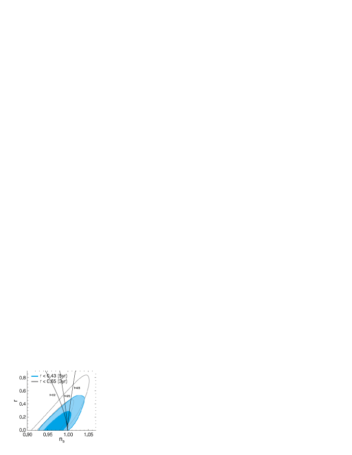
Figure 1: The plot shows $r$ versus $n_{s}$. Here, we have used the WMAP five-year data where $P_{\cal R}(k_{*})\simeq 2.4\times 10^{-9}$, together with $\beta=10^{10}m_{p}^{-6}$. The five-year WMAP data places stronger limits on r (shown in blue) than three-year data (grey)astro .

Figure 2: The plot shows $n_{run}=d\ln n_{s}/d\ln k$ versus $n_{s}$. Here, we have used the WMAP five-year data where $P_{\cal R}(k_{*})\simeq 2.4\times 10^{-9}$, together with the value $\beta=10^{10}m_{p}^{-6}$. Models with no tensor contribution, and with a tensor contribution marginalized over, are shownastro .

IV Conclusions

In this paper we have studied the brane-intermediate inflationary model in the high-energy scenario. We have found an exact solution of the Friedmann equations for a flat universe containing a scalar field $\phi(t)$ with potential $V(\phi)$. In the slow-roll approximation we have found a general relation between the scalar potential and its derivative. We have also obtained explicit expressions for the corresponding, power spectrum of the curvature perturbations $P_{\cal R}$, tensor-scalar ratio $r$, scalar spectrum index $n_{s}$ and its running $n_{run}$.

By using the scalar potential (see Eq.(10)) and from the WMAP five year data, we have found constraints on the parameter $A$ for a given values of $\beta$ and $f$. In order to bring some explicit results we have taken the constraint $r-n_{s}$ plane to first-order in the slow roll approximation. We noted that the parameter $f$, which lies in the range $1>f>0$, the model is well supported by the data as could be seen from Fig.(1). Here, we have used the WMAP five year data, where $P_{\cal R}(k_{*})\simeq 2.4\times 10^{-9}$, and we have taken the value $\beta=10^{10}m_{p}^{-6}$. On the other hand, Fig.(2) clearly shows that for the value of $f>4/5$ allows $n_{s}>1$. However, from Fig.(2) the best values of $f$ occurs when it lies in the range $4/5>f>2/3$.

In this paper, we have not addressed the phenomena of reheating and possible transition to the standard cosmology (see e.g., Refs.SRc ; u ; yo ). A possible calculation for the reheating temperature in the hight-energy scenario would give new constrains on the parameters of the model. We hope to return to this point in the near future.

- (1) A. Guth, Phys. Rev. D 23, 347 (1981).
- (2) A. Albrecht and P. J. Steinhardt, Phys. Rev. Lett. 48, 1220 (1982); A complete description of inflationary scenarios can be found in the book by A. Linde , Particle physics and inflationary cosmology (Gordon and Breach, New York, 1990).
- (3) J. Dunkley et al. [WMAP Collaboration], arXiv:0803.0586 [astro-ph]
- (4) G. Hinshaw et al., arXiv:0803.0732 [astro-ph]; M. R. Nolta et al. [WMAP Collaboration], arXiv:0803.0593 [astro-ph].
- (5) A. Sen, JHEP 0204, 048 (2002).
- (6) K. Akama, Lect. Notes Phys. 176, 267 (1982); V. A. Rubakov and M. E. Shaposhnikov, Phys. Lett. B 159, 22 (1985); N. Arkani- Hamed, S. Dimopoulos, and G. Dvali, Phys. Lett. B 429, 263 (1998); M. Gogberashvili, Europhys. Lett. 49, 396 (2000); L. Randall and R. Sundrum, Phys. Rev. Lett. 83, 3370 (1999); 83, 4690 (1999).
- (7) T. Shiromizu, K. Maeda, and M. Sasaki, Phys. Rev. D 62, 024012 (2000).
- (8) P. Bin etruy, C. Deffayet, and D. Langlois, Nucl. Phys. B565, 269 (2000) ; P. Bin etruy, C. Deffayet, U. Ellwanger, and D. Langlois, Phys. Lett. B 477, 285 (2000).
- (9) R. Maartens, D. Wands, B. A. Bassett, and I. P. C. Heard, Phys. Rev. D 62, 041301 (2000).
- (10) J. M. Cline, C. Grojean, and G. Servant, Phys. Rev. Lett.83, 4245 (1999); C. C saki, M. Graesser, C. Kolda, and J. Terning, Phys. Lett. B 462, 34 (1999); D. Ida, JHEP 0009, 014 (2000); R. N. Mohapatra, A. P erez-Lorenzana, and C. A. de S. Pires, Phys. Rev. D 62, 105030 (2000); R. N. Mohapatra, A. P erez-Lorenzana, and C. A. de S. Pires, Int. J. Mod. Phys. A 16, 1431 (2001); Y. Gong, arXiv:gr-qc/0005075.
- (11) R. Maartens, arXiv:gr-qc/0101059.
- (12) J. D Barrow, Phys. Lett. B 235, 40 (1990); J. D Barrow and P. Saich, Phys. Lett. B 249, 406 (1990);A. Muslimov, Class. Quantum Grav. 7, 231 (1990); A. D. Rendall, Class. Quantum Grav. 22, 1655 (2005).
- (13) J. D Barrow and A. R. Liddle, Phys. Rev. D 47, R5219 (1993); A. Vallinotto, E. J. Copeland, E. W. Kolb, A. R. Liddle and D. A. Steer, Phys. Rev. D 69, 103519 (2004); A. A. Starobinsky JETP Lett. 82, 169 (2005).
- (14) W. H. Kinney, E. W. Kolb, A. Melchiorri and A. Riotto, Phys. Rev. D 74, 023502 (2006); J. Martin and C. Ringeval JCAP 08 (2006); F. Finelli, M. Rianna and N. Mandolesi, JCAP 12 006 (2006).
- (15) J. D. Barrow, A. R. Liddle and C. Pahud, Phys. Rev. D, 74, 127305 (2006).
- (16) D. G. Boulware and S. Deser, Phys.Rev. Lett. 55, 2656 (1985); Phys. Lett. B 175, 409 1986).
- (17) T. Kolvisto and D. Mota, Phys. Lett. B 644, 104 (2007); Phys. Rev. D. 75, 023518 (2007).
- (18) I. Antoniadis, J. Rizos and K. Tamvakis, Nucl.Phys. B 415, 497 (1994).
- (19) S. Mignemi and N. R. Steward, Phys. Rev. D 47, 5259 (1993); P. Kanti, N. E. Mavromatos, J. Rizos, K. Tamvakis and E. Winstanley, Phys. Rev. D 54, 5049 (1996); Ch.-M Chen, D. V. Gal tsov and D. G. Orlov, Phys. Rev. D 75, 084030 (2007).
- (20) S. Nojiri, S. D. Odintsov and M. Sasaki, Phys. Rev. D 71, 123509 (2004); G. Gognola, E. Eizalde, S. Nojiri, S. D. Odintsov and E. Winstanley, Phys. Rev. D 73, 084007 (2006).
- (21) A. K. Sanyal, Phys. Lett. B, 645,1 (2007).
- (22) A. Kamenshchik, U. Moschella and V. Pasquier, Phys. Lett. B 511, 265 (2001); N. Bilic, G. B. Tupper and R. D. Viollier, Phys. Lett. B 535, 17 (2002).
- (23) J. M. Cline, C. Grojean and G. Servant, Phys. Rev. Lett. 83, 4245 (1999)
- (24) S. Tsujikawa, D. Parkinson and B. A. Bassett, Phys. Rev. D 67, 083516 (2003).
- (25) D. Langlois, R. Maartens and D. Wands, Phys. Lett. B 489, 259 (2000).
- (26) M. Tegmark et al., Phys. Rev. D 69, 103501 (2004).
- (27) D. N. Spergel et al. [WMAP Collaboration], Astrophys. J. Suppl. 170, 377 (2007).
- (28) S. del Campo and R. Herrera, Phys. Rev. D 76, 103503 (2007).
- (29) E. J. Copeland, A. R. Liddle and J. E. Lidsey, Phys. Rev. D 64, 023509 (2001); E. J. Copeland and O. Seto, Phys. Rev. D 72, 023506 (2005).
- (30) C. Campuzano, S. del Campo and R. Herrera, JCAP 0606, 017 (2006); C. Campuzano, S. del Campo and R. Herrera, Phys. Lett. B 633, 149 (2006); C. Campuzano, S. del Campo and R. Herrera, Phys. Rev. D 72, 083515 (2005) [Erratum-ibid. D 72, 109902 (2005)].