Bubble formation in $\phi^{6}$ potential

Abstract: Scalar field theory with an asymmetric potential is studied at zero temperature and high-temperature for $\phi^{6}$ potential. The equations of motion are solved numerically to obtain O(4) spherical symmetric and O(3) cylindrical symmetric bounce solutions. These solutions control the rates for tunneling from the false vacuum to the true vacuum by bubble formation. The range of validity of the thin-wall approximation (TWA) is investigated. An analytical solution for the bounce is presented, which reproduces the action in the thin-wall as well as the thick-wall limits.

keywords: phase transition, tunneling, scalar field theory

1 Introduction

The problem of decay of a metastable state via quantum tunneling has important applications in many branches of physics, from condensed matter to particle physics and cosmology. The tunneling is not a perturbative effect. In the semi-classical approximation, the decay rate per unit volume is given by an expression of the form

$$\Gamma\quad=\quad A\quad e^{-S_{E}},$$ (1)

where $S_{E}$ is the Euclidean action for the bounce: the classical solution of the equation of motion with appropriate boundary conditions. The bounce has turning points at the configurations at which the system enters and exits the potential barrier, and analytic continuation to Lorentzian time at the exit point gives us the configuration of the system at that point and its subsequent evolution. The solution of the equation of motion looks like a bubble in four dimensional Euclidean space with radius R and thickness proportional to the coefficient of the symmetry breaking term in the potential. When there are more than one solution satisfying the boundary conditions, the one with the lowest $S_{E}$ dominates equation (1). The prefactor A comes from Gaussian functional integration over small fluctuations around the bounce. The zero-temperature formalism is well-developed [1, 2, 3]. In particular, it has been proved rigorously that the least action is given by the bounce which is O(4) invariant [3].

Linde [4] extended the formalism to finite temperatures. He suggested that at temperatures much smaller than the inverse radius of the bubble at zero-temperature, the bounces are periodic in the Euclidean time $\tau$ direction and widely separated. Beyond this temperature they start merging into one another producing what is known as “wiggly cylinder” solutions. As one keeps increasing the temperature these wiggles smoothly straighten out, and the solution goes into an O(3) invariant cylinder (independent of Euclidean time $\tau$) solution that dominates the thermal activation regime.

A numerical and analytical calculations of the first and second order phase transitions has been considered by many authors. For example, an analytical calculation of the nucleation rate for first order phase transitions beyond the TWA for the standard Ginzburg-Landau potential with $\phi$ asymmetric term has been studied by M$\ddot{\rm u}$nster and Rotsch [5]. We have considered in an earlier work the $\phi^{4}$ theory with different symmetry breaking terms [6], where we have obtained numerical as well as analytical solution for different values of the asymmetric term. In this paper we consider $\phi^{6}$ potential motivated by the recent work on baryon asymmetry in the standard model with a low cut-off [7]. Also, if the Higgs potential is stabilized by a $\phi^{6}$ interaction, a strong first order transition can occur for Higgs masses well above $100$ Gev [8, 9, 10]. Moreover, the $\phi^{6}$ potential has been investigated by many authors in the context of condensed matter as well as particle physics (see for example [11, 12, 13, 14, 15, 16, 17, 18]).

The general form of the potential is

$$U(\phi)={1\over 2}m^{2}\phi^{2}+\lambda\phi^{4}+g\phi^{6},$$ (2)

which has a second-order transition in $m^{2}$ if $\lambda>0$ by ignoring corrections due to fluctuations, a first-order transition in $m^{2}$ if $\lambda<0$, and a tricritical point at $\lambda=0$ [15]. Since we are interested in the case of getting bounce solution, so we take the case of $\lambda<0$. Following [11], we rewrite the potential $U(\phi)$ in terms of the parameters $\phi_{0}$ and $\delta$ such that

$$U(\phi)=g\,\phi^{2}(\phi^{2}-\phi_{0}^{2})^{2}-\delta\phi^{2},$$ (3)

where $\phi_{0}^{2}=-\lambda/{2g}$ and $\delta=(\lambda^{2}/g-2m^{2})/4$. Looking carefully to the potential, we realize that by fixing $\lambda$ and $g$, then $\delta$ is changed by changing the value of $m^{2}$. Hence the $\delta$ term plays the asymmetric part of the potential and is responsible for the first-order feature of the phase transition, by causing the coexistence of two minima (false and true) separated by a barrier. So, for different values of $\delta$, we get different shape of the potential.

An interesting special case is the so called thin-wall approximation (TWA), when the bubble radius $R$ is much larger than the thickness of the bubble wall and the barrier between the two minima is large. In this limit ($\delta\rightarrow 0$), there is an analytical formula for $S_{E}$ in terms of the wall surface energy, and the details of the field theory are unimportant. However, it would be nice to also have an analytical interpolating form for the solution itself. Also, it is not clear a priori what the limit of validity of the TWA is. Another interesting case is called the thick wall which is reached when the barrier is small. One can easily show that the barrier is completely disappeared when $\delta=g\phi_{0}^{4}$ and in this case there is no bubbles formed and the field goes from the false vacuum to the true vacuum without tunneling.

In this paper we address the above issues. We obtain accurate numerical solutions for the zero-temperature and high-temperature bounces for $\phi^{6}$ theory with $\phi^{2}$ symmetry-breaking term. We compute the actions in each case, and find that, for a modest value of the asymmetric coupling $\delta(=0.1)$, the action given by TWA formula agrees to within $12.8\%$ with that obtained from the numerical solution. We test the criterion for the goodness of TWA, in terms of the temperature $T_{\beta}$ at which the actions of the O(4) and O(3) solutions become equal [6]. A numerical investigation shows that the TWA holds up to $\delta\sim 0.25$. Finally, we present an analytical solution which satisfies the equation of motion with parameters fixed by demanding stationary action. This reproduces TWA results very well and, in the thick-wall limit, is in good agreement with the numerical results.

2 Bubble formation

Let us consider a scalar field theory with a Lagrangian density

$$\mathcal{L}(\phi)={1\over 2}({\partial_{\mu}\phi})^{2}-U(\phi),$$ (4)

where the potential $U(\phi)$ has two minima at $\phi_{-}$ (false vacuum) and $\phi_{+}$ (true vacuum).

In the semi-classical approximation the barrier tunneling leads to the appearance of bubbles of a new phase with $\phi=\phi_{+}$ as classical solutions in Euclidean space (i.e., imaginary time $\tau$). To calculate the probability of such a process in quantum field theory at zero temperature, one should first solve the Euclidean equation of motion :

$$\partial_{\mu}\partial_{\mu}\phi={dU(\phi)\over d\phi},$$ (5)

with the boundary condition $\phi\to\phi_{-}$ as $\vec{x}^{2}+\tau^{2}\to\infty$ , where $\tau$ is the imaginary time. The probability of tunneling per unit time per unit volume is given by

$$\Gamma=A\quad e{{}^{-S_{E}[\phi]}},$$ (6)

where $S_{E}[\phi]$ is the Euclidean action corresponding to the solution of equation (5) and given by the following expression :

$$S_{E}[\phi]=\int d^{4}{x}\left[{1\over 2}({\partial\phi\over\partial\tau})^{2}+{1\over 2}(\nabla\phi)^{2}+U(\phi)\right].$$ (7)

It is sufficient to restrict ourselves to the O(4) symmetric solution $\phi(\vec{x}^{2}+\tau^{2})$ , since it is this solution that provides the minimum of the action $S_{E}[\phi]$ [3]. In this case equation (5) takes the simpler form

$${d^{2}\phi\over d\rho^{2}}+{3\over\rho}{d\phi\over d\rho}={dU(\phi)\over d\phi},$$ (8)

where $\rho=\sqrt{\vec{x}^{2}+\tau^{2}}$, with boundary conditions

$$\phi\to\phi_{-}\quad{\rm as}\quad\rho\to\infty,\quad{d\phi\over d\rho}=0\quad{\rm at}\quad\rho=0.$$ (9)

We denote the action of this solution by $S_{4}$.

Now let us consider the finite temperature case. Following [4], in the calculation of the action $S_{E}(\phi)$ the integration over $\tau$ is reduced simply to multiplication by $T^{-1}$, i.e., $S_{E}[\phi]=T^{-1}\>S_{3}[\phi]$. Here $S_{E}[\phi]$ is the four-dimensional action and $S_{3}[\phi]$ is the three-dimensional action corresponding to the O(3)-symmetric bubble and given by :

$$S_{3}[\phi]=\int d^{3}r\left[{1\over 2}{(\nabla\phi)^{2}}+U(\phi,T)\right].$$ (10)

To calculate $S_{3}(\phi)$ it is necessary to solve the equation

$${d^{2}\phi\over dr^{2}}+{2\over r}{d\phi\over dr}={dU(\phi,T)\over d\phi}$$ (11)

with boundary conditions

$$\phi\to\phi_{-}\quad{\rm as}\quad r\to\infty,\quad{d\phi\over dr}=0\quad{\rm at}\quad r=0.$$ (12)

where $r=\sqrt{\vec{x}^{2}}$. The complete expression for the probability of tunneling per unit time per unit volume in the high-temperature limit ($T>>R^{-1}$) is obtained in analogy to the one used in [2] and is given by:

$$\Gamma(T)=A(T)\>e^{-S_{3}[\phi,T]/T}.$$ (13)

In the theory of bubble formation , the interesting quantity to calculate is the probability of decay between $\phi=\phi_{-}$ and $\phi=\phi_{+}$ which are the two minima of $U(\phi)$. There is an interesting case (in the sense that the action can be calculated analytically) when $U(\phi_{+})-U(\phi_{-})=\varepsilon$ is much smaller than the height of the barrier. This is known as the thin-wall approximation (TWA). At $T=0$, in the TWA limit, the action $S_{4}$ of the O(4)-symmetric bubble is equal to

$$S_{4}={{27\pi^{2}S_{1}^{4}}\over{2\varepsilon^{3}}}.$$ (14)

Here $S_{1}$ is the bubble wall surface energy (surface tension), given by

$$S_{1}=\int_{0}^{\infty}d\rho\left[({d\phi\over d\rho})^{2}+U(\phi)\right],$$ (15)

and the integral should be calculated in the limit $\varepsilon\to 0$. The bubble radius $R$ is written in terms of $S_{1}$ and $\varepsilon$ as

$$R={{3S_{1}}\over\varepsilon}.$$ (16)

The results presented above were obtained by Coleman [2].

These results can be easily extended to the case $T>>R^{-1}$ [4]. To this end it is sufficient to take into account that

$$S_{3} = 4\pi\int_{0}^{\infty}dr\>r^{2}\left[{1\over 2}({d\phi\over dr})^{2}+U(\phi,T)\right]$$ (17)

$$= {-{4\over 3}}\varepsilon\pi R(T)^{3}+4\pi R(T)^{2}S_{1}(T),$$

where $S_{1}(T)$ is the bubble wall surface energy (surface tension) at finite temperature and is given by:

$$S_{1}(T)=\int_{0}^{\infty}dr\left[({d\phi\over dr})^{2}+U(\phi,T)\right].$$ (18)

As before, the integral should be calculated in the limit $\varepsilon\to 0$.

The bubble radius $R(T)$ is calculated by minimizing $S_{3}$ with respect to $R(T)$ and this gives us

$$R(T)={{2S_{1}(T)}\over\varepsilon},$$ (19)

whence it follows that

$$S_{3}={{16\pi S_{1}^{3}(T)}\over{3\varepsilon^{2}}}.$$ (20)

3 Numerical results

For O(4) symmetry at $T=0$, equation (7) reduces to

$$S_{4}=2\pi^{2}\int_{0}^{\infty}d\rho\>\rho^{3}\left[{1\over 2}({d\phi\over d\rho})^{2}+U(\phi)\right].$$ (21)

We compute the action for different values of the parameter $\delta$ in the symmetry-breaking term in the potential $U(\phi)$, equation (3), which reads as

$$S_{4}=2\pi^{2}\int_{0}^{\infty}d\rho\>\rho^{3}\left[{1\over 2}({d\phi\over d\rho})^{2}+g\,\phi^{2}(\phi^{2}-\phi_{0}^{2})^{2}-\delta\phi^{2}\right].$$ (22)

Following [11], we assume $\phi_{0}=2.39$ and $g=0.07$, then the only adjustable parameter in the Lagrangian is $\delta$. So, by covering the whole range $0<\delta<g\phi_{0}^{4}$ we should be covering all relevant cases.

The equation of motion is now

$${d^{2}\phi\over d\rho^{2}}+{3\over\rho}{d\phi\over d\rho}=6g\phi^{5}-8g\phi_{0}^{2}\phi^{3}+2(g\phi_{0}^{4}-\delta)\phi,$$ (23)

and the boundary conditions are

$$\phi=0\quad{\rm as}\quad\rho\to\infty,\quad{d\phi\over d\rho}=0\quad{\rm at}\quad\rho=0.$$ (24)

By solving equation (23) numerically for different values of $\delta$, substituting the solution in equation (22) and integrating, we obtain the action for each value of $\delta$.

At high temperature, we look for the O(3) symmetric solution with cylindrical symmetry. Then equation (10) takes the form

$$S_{3}=4\pi\int_{o}^{\infty}dr\>r^{2}\left[{1\over 2}({d\phi\over dr})^{2}+g\,\phi^{2}(\phi^{2}-\phi_{0}^{2})^{2}-\delta\phi^{2}\right].$$ (25)

The equation of motion is then

$${d^{2}\phi\over dr^{2}}+{2\over r}{d\phi\over dr}=6g\phi^{5}-8g\phi_{0}^{2}\phi^{3}+2(g\phi_{0}^{4}-\delta)\phi,$$ (26)

and the boundary conditions are

$$\phi=0\quad{\rm as}\quad r\to\infty,\quad{d\phi\over dr}=0\quad{\rm at}\quad r=0.$$ (27)

Again, we solve equation (26) numerically for different values of $\delta$, substitute the solution in equation (25) and integrate to obtain the action for each $\delta$. Figure 1 shows the bubble profile for different values of $\delta$. Note that the value of the scalar field $\phi$ inside the bubble decreases with $\delta$. In figure 2 we have plotted this value together with the minimum of the potential $U(\phi)$. At $\delta=0$ the value of $\phi_{0}$, i.e. $\phi(r=0)$, coincides with the minimum of the potential $\phi_{m}$. However, as $\delta$ decreases, the minimum increases while $\phi_{0}$ initially increased then it decreases and moves away from the minimum of $U(\phi)$. Same behavior has been obtained and explained by [19] and it is due the decreasing of the height of the potential and the increasing in the energy difference between minima. So, physically this means that as the barrier between minima disappears, it becomes easier to from a large bubble with a small value of $\phi$ inside it. Same result can been obtained also for the case of zero temperature.

Table 1. Numerical values of the action $T=0$ and high temperature for different values of the asymmetry parameter $\delta$.

$\delta$	$S_{4}$ (Numerical)	$S_{3}$ (Numerical)
0.1	70978.1	1620.08
0.2	9739.27	441.89
0.29	3625.65	225.41
0.4	1519.96	127.73
0.6	523.12	63.36
0.8	253.85	38.72
1.0	143.42	26.27
1.2	91.07	18.98
1.4	60.85	14.08
1.6	42.67	10.43
1.8	30.03	7.79
2.0	21.34	5.53
2.2	15.01	3.52
2.28	12.84	2.89

As we discussed in the introduction, for small values of $\delta$ we can use the TWA formula for computing the action. From equation (15)

$$S_{1} = \int_{0}^{\infty}dr\left[({d\phi\over dr})^{2}+g\,\phi^{2}(\phi^{2}-\phi_{0}^{2})^{2}\right]$$ (28)

$$= -\int_{0}^{\phi_{0}}d\phi\>\sqrt{2g\,\phi^{2}(\phi^{2}-\phi_{0}^{2})^{2}}$$

$$= {3.05},$$

for $\phi_{0}=2.39$ and $g=0.07$, see [11]. The radius is given by

$$R={{3S_{1}}\over\varepsilon},$$ (29)

where $\varepsilon=\phi_{0}^{2}\,\delta$ (see [2, 11]). For $\delta=0.1$, we have $R=16.02$ and the value of the action is (see equation (14))

$$S_{4}=61918.4.$$ (30)

Comparing this analytical value with the numerical one for $\delta=0.1$, we get an error equal $12.8\%$. In [11], the authors choose $\delta=0.29$ to represents the TWA and they have concluded that it is not a good value to be taken. This is also confirmed by our calculations where we get an error approximately $30\%$.

At high temperature, again $S_{1}=3.05$. The value of $R(T)=10.68$ at $\delta=0.1$ and the action is (see equation (20))

$$S_{3}(T)=1454.26.$$ (31)

Comparing this analytical value with the numerical one for $\delta=0.1$, we get an error equal $10.24\%$. Thus even for $\delta$ as small as $0.1$ the TWA formula for the action does not give very accurate results. Obviously, there is no point in comparing numerical results obtained for higher values of $\delta$ with the TWA formula.

To test our numerical method (we have used Hamming’s modified predictor-corrector method for solving the equation of motion), we have calculated the action $S_{4}$ for small values of the symmetry breaking parameter $\delta$ in the potential and compared it with the TWA formula. In figure 3, we plot the percentage error in the TWA formula as a function of $\delta$. The crosses represent our results while the solid line shows a fit to the data. We see that the error decreases for small $\delta$, as expected, and approaches zero as $\delta\rightarrow 0$.

As already mentioned, at zero temperature the O(4) symmetric solution has the lowest value of $S_{E}$, i.e., $S_{E}=S_{4}$. At high temperature, we have $S_{E}=S_{3}/T$. At intermediate temperatures other solutions exist. In the TWA, however, it has been shown [20] that all other solutions have higher Euclidean action. This corresponds to a first order phase transition from quantum tunneling at low temperature to thermal hopping at high temperatures. The transition temperature $T_{\beta}$ is given by equating $S_{4}$ with $S_{3}/T$, i.e.,

$$T_{\beta}={S_{3}\over S_{4}}$$ (32)

If the surface tension $S_{1}$ is temperature independent, we have

$$S_{4}={{27\pi^{2}S_{1}^{4}}\over{2\varepsilon^{3}}}$$ (33)

$$S_{3}={{16\pi S_{1}^{3}}\over{3\varepsilon^{2}}}$$ (34)

Dividing equation (33) by equation (34) and putting $\varepsilon=\phi_{0}^{2}\,\delta$ (see [2]) we get

$$T_{\beta}=C*\delta$$ (35)

where

$$C={32\,\phi_{0}^{2}\over{81\pi S_{1}}}$$ (36)

Thus we see that, in the TWA, $T_{\beta}$ increases linearly with $\delta$. We test this by computing $S_{3}/S_{4}$ from our numerical solutions at different values of $\delta$. Figure 4 shows our results for the potential given by equation (3). We see that, for $\delta\leq 0.2$, there is very good agreement with the predicted linear dependence. This also confirms that, in the domain of validity of the TWA, the surface tension $S_{1}(T)$ is independent of $T$. Beyond $\delta\sim 0.2$ in our dimensionless units, there is a systematic deviation from linearity. Thus we can say that, for values of $\delta$ larger than this, the wall thickness becomes important. Same behavior has been obtained also in our earlier work [6].

4 Analytic solution for zero temperature

We calculate the action analytically in two extreme limits: the thin-wall and thick-wall using the potential given by equation (3).

Thin-wall limit : $\delta\to 0$

In an earlier paper [6], we have found that an analytic solution for the bounce of the form of a Fermi function:

$$\phi(\rho)={\gamma\over e^{{{(\rho^{2}-R^{2})}/\Lambda^{2}}}+1}$$ (37)

is a good approximation for the $\phi^{4}$ theory. But it has been shown that for the $\phi^{6}$ potential, the analytic solution for the bounce has the form [13, 14]

$$\phi_{\rm wall}^{2}(\rho)=\frac{\phi_{0}^{2}}{1+e^{\mu\rho}},$$ (38)

where $\mu=\sqrt{8g}\phi_{0}^{2}=4.21$, and $\mu^{2}$ is the second derivative of the potential in the TWA limit evaluated at $\phi_{0}$. So, motivated by the above results, we assume

$$\phi^{2}(\rho)={\gamma\over e^{{{(\rho^{2}-R^{2})}/\Lambda^{2}}}+1},$$ (39)

where $\rho=\sqrt{\vec{x}^{2}+\tau^{2}}$, $R$ is the radius of the bubble and $\Lambda$ its width, acts like a bounce in the TWA and leads to the correct value for the action $S_{4}$. The parameter $\sqrt{\gamma}$ is approximately equal to true minimum in the TWA. The bounce has values $\phi=\sqrt{\gamma}$ at $\rho=0$ and $0$ at $\rho\to\infty$. The boundary conditions (9) are satisfied by equation (39).

To evaluate $\gamma$, $R$, and $\Lambda$, we substitute the ansatz (39) in equation (23) :

$${d^{2}\phi\over d\rho^{2}}+{3\over\rho}{d\phi\over d\rho}=6g\phi^{5}-8g\phi_{0}^{2}\phi^{3}+2(g\phi_{0}^{4}-\delta)\phi.$$ (40)

Then the left-hand side (L.H.S.) and the right-hand side (R.H.S.) are respectively

$$L.H.S.={({3\rho^{2}/\Lambda^{4}})\sqrt{\gamma}\over(e^{{{(\rho^{2}-R^{2})}/\Lambda^{2}}}+1)^{5/2}} + {{(-4\rho^{2}/\Lambda^{4}+4/\Lambda^{2})\sqrt{\gamma}}\over(e^{{{(\rho^{2}-R^{2})}/\Lambda^{2}}}+1)^{3/2}}$$ (41)

$$+ {{(\rho^{2}/\Lambda^{4}-4/\Lambda^{2})\sqrt{\gamma}}\over(e^{{{(\rho^{2}-R^{2})}/\Lambda^{2}}}+1)^{1/2}}.$$

$$R.H.S.={{6g\gamma^{5/2}}\over(e^{{{(\rho^{2}-R^{2})}/\Lambda^{2}}}+1)^{5/2}} - {{8g\phi_{0}^{2}\gamma^{3/2}}\over(e^{{{(\rho^{2}-R^{2})}/\Lambda^{2}}}+1)^{3/2}}$$ (42)

$$+ {{2(g\phi_{0}^{4}-\delta)\sqrt{\gamma}}\over(e^{{{(\rho^{2}-R^{2})}/\Lambda^{2}}}+1)^{1/2}}.$$

In the TWA, the solution is constant except in a narrow region near the wall at $\rho=R$. So, we replace in equation (41)

$$\mathrm{{3\rho^{2}\over\Lambda^{4}}\,\,\,by\,\,\,{{3R^{2}}\over\Lambda^{4}}(1-a\Lambda^{2}/R^{2})\,\,\,in\,\,\,the\,\,\,{1\over(e^{{{(\rho^{2}-R^{2})}/\Lambda^{2}}}+1)^{5/2}}\,\,\,term},$$ (43)

$$\mathrm{{4\over\Lambda^{2}}-{4\rho^{2}\over\Lambda^{4}}\,\,\,by\,\,\,{-}{{4R^{2}}\over\Lambda^{4}}(1-b\Lambda^{2}/R^{2})\,\,\,in\,\,\,the\,\,\,{1\over(e^{{{(\rho^{2}-R^{2})}/\Lambda^{2}}}+1)^{3/2}}\,\,\,term},$$ (44)

$$\mathrm{{\rho^{2}\over\Lambda^{4}}-{4\over\Lambda^{2}}\,\,\,by\,\,\,{{R^{2}}\over\Lambda^{4}}(1-c\Lambda^{2}/R^{2})\,\,\,in\,\,\,the\,\,\,{1\over(e^{{{(\rho^{2}-R^{2})}/\Lambda^{2}}}+1)^{1/2}}\,\,\,term},$$ (45)

where $a$, $b$ and $c$ are parameters to be determined later.

Comparing equation (41) with equation (42) in the range $R^{2}(1-\Lambda^{2}/R^{2})=R^{2}-\Lambda^{2}<\rho^{2}<R^{2}+\Lambda^{2}=R^{2}(1+\Lambda^{2}/R^{2})$ where $\rho^{2}\simeq R^{2}$ as $\Lambda^{2}/R^{2}<<1$ , we have :

$$2g\gamma^{2}={{R^{2}}\over\Lambda^{4}}(1-a\Lambda^{2}/R^{2}),$$

$$2g\phi_{0}^{2}\gamma={{R^{2}}\over\Lambda^{4}}(1-b\Lambda^{2}/R^{2}),$$ (46)

$$2(g\phi_{0}^{4}-\delta)={{R^{2}\over\Lambda^{4}}(1-c\Lambda^{2}/R^{2})},$$

We can now evaluate the zero-temperature action $S_{4}$ :

$$S_{4}=2\pi^{2}\>\int_{0}^{\infty}d\rho\>\rho^{3}\left[{1\over 2}({d\phi\over d\rho})^{2}+U(\phi)\right].$$ (47)

Substituting equation (39) in equation (47) and integrating we get

$$S_{4} = 2\pi^{2}R^{4}\gamma\Bigg{[}{1\over{8\Lambda^{2}}}+{1\over{4R^{2}}}+{\pi^{2}\Lambda^{2}\over 24R^{2}}+(g\phi_{0}^{4}-\delta)\left({1\over 4}+{\pi^{2}\Lambda^{4}\over 12R^{4}}\right)$$ (48)

$$-{1\over 2}g\phi_{0}^{2}\gamma\left(1-{{2\Lambda^{2}}\over R^{2}}+{\pi^{2}\Lambda^{4}\over 3R^{4}}\right)$$

$$+{g\over 4}\gamma^{2}\left(1-{{3\Lambda^{2}}\over{R^{2}}}+({\pi^{2}\over 3}+1){\Lambda^{4}\over R^{4}}\right)\Bigg{]}.$$

We now determine the parameters $a$, $b$, and $c$ by demanding ${dS_{4}/dR}={dS_{4}/d\Lambda}={dS_{4}/d\gamma}=0$. Differentiating equation (48) and using equation (46), we find that to leading order in $\Lambda^{2}/R^{2}$,

$$3-2a+4b-2c=0,$$

$$2+3a-4b=0,$$ (49)

$$-3a+4b-c=0,$$

which leads to $a=-1$, $b=-1/4$ and $c=2$. Using equation (46), we can rewrite equation (48) as :

$$S_{4} = {\pi^{2}\over g\phi_{0}^{2}}{R^{6}\over\Lambda^{6}}\Bigg{[}\left(\frac{1}{4}-\frac{a}{8}+\frac{b}{4}-\frac{c}{8}\right)+\left(\frac{7}{16}+\frac{11a}{32}-\frac{7b}{16}-\frac{c}{32}\right)\frac{\Lambda^{2}}{R^{2}}$$ (50)

$$+\left(\frac{3}{32}+\frac{\pi^{2}}{24}-\frac{a}{32}-\frac{\pi^{2}a}{24}-\frac{b}{8}+\frac{\pi^{2}b}{12}-\frac{\pi^{2}c}{24}\right){\Lambda^{4}\over R^{4}}$$

$$+\left(\frac{\pi^{2}}{96}-\frac{a}{32}-\frac{\pi^{2}a}{96}+\frac{\pi^{2}b}{48}-\frac{\pi^{2}c}{96}\right)\frac{\Lambda^{6}}{R^{6}}+O(\frac{\Lambda^{8}}{R^{8}})\Bigg{]},$$

This gives

$$S_{4}={\pi^{2}\over g\phi_{0}^{2}}{R^{6}\over\Lambda^{6}}\left(0.063+0.141\frac{\Lambda^{2}}{R^{2}}-0.049\frac{\Lambda^{4}}{R^{4}}-0.020\frac{\Lambda^{6}}{R^{6}}+O(\frac{\Lambda^{8}}{R^{8}})\right).$$ (51)

The quantities $\gamma$, $R$ and $\Lambda$ are determined from equation (46) using the values of $a$, $b$, and $c$. So we have

$$2g\gamma^{2}-2g\phi_{0}^{2}\gamma\left({{c-a\over{c-b}}}\right)+2(g\phi_{0}^{4}-\delta)\left({{b-a\over c-b}}\right)=0,\\$$ (52)

which gives

$${R^{2}\over\Lambda^{2}}={{g\phi_{0}^{2}c\gamma-b(g\phi_{0}^{4}-\delta)}\over{g\phi_{0}^{2}\gamma-(g\phi_{0}^{4}-\delta)}},$$ (53)

and

$$\Lambda^{2}={{b-a}\over{2g\gamma^{2}-2g\phi_{0}^{2}\gamma}}={{{c-b}\over{2g\phi_{0}^{2}\gamma-2(g\phi_{0}^{4}-\delta})}},$$ (54)

with $\gamma$ given by equation (52). We have then, for $\delta=0.1$, $\gamma=5.83$, which implies that $R^{2}/\Lambda^{2}=35.1$, $R=16.3$, $\Lambda=2.75$ and $S_{4}=70997.3$. Comparing these results with the TWA formulae, we find that the departure of the radius from the TWA is $R/R_{TWA}=1.02$ while the departure of the action is ${S_{4}/S_{TWA}}=1.14$, which is a fairly good result. On the other hand, there is no departure of the radius as well as the action from the numerical values at $\delta=0.1$ which is an excellent result. Table 2 shows our numerical as well as the analytical values of the action and the radius for different values of $\delta$. We have calculated the numerical value of the radius when the derivative of the filed is maximum while in [19] the author has calculated the radius in a different way.

Table 2. Numerical and analytical values of the action and the radius for different values of $\delta$.

$\delta$	$S_{4}$ (Numerical)	$S_{4}$ (Analytical)	$R$ (Numerical)	$R$ (Analytical)
0.1	70978.1	70997.3	16.3	16.3
0.2	9739.27	10008.3	8.3	8.28
0.29	3625.65	3622.26	5.8	5.79
0.4	1519.96	1540.44	4.2	4.26
0.6	523.12	543.96	2.86	2.9
0.8	253.85	266.95	2.2	2.22
1.0	143.42	156.01	1.82	1.81
1.2	91.07	101.54	1.53	1.53
1.4	60.85	70.97	1.32	1.33

Notice that there is an excellent agreement between the radii while actions are fairly agree till $\delta=1.0$. So, we conclude that our ansatz gives us far better results than the TWA formula. In figure 5 we compare our numerical result with the analytic one for $\delta=0.1$. From the figure we see that the Fermi function agrees very well with our numerical results

Thick-wall limit: $\delta\to g\phi^{4}_{0}$

The form of the bounce in equation (39) suggests that the thick wall limit, which would correspond to small values of $R^{2}/\Lambda^{2}$, would be obtained by approximating the Fermi function by the Maxwell-Boltzmann function, which leads to a Gaussian:

$$\phi^{2}(\rho)=\gamma e^{-\rho^{2}/\Lambda^{2}}.$$ (55)

The action for this form of bounce is found to be

$$S_{4}={2{\pi^{2}\Lambda^{4}\gamma}}\Bigg{[}{1\over{2\Lambda^{2}}}+{g\over 18}\gamma^{2}-{1\over 4}g\phi_{0}^{2}\gamma+{1\over 2}(g\phi_{0}^{4}-\delta)\Bigg{]}.$$ (56)

Equations (46) then reduce to

$$2g\gamma^{2}=-{a\over\Lambda^{2}}~{},\quad 2g\phi_{0}^{2}\gamma=-{b\over\Lambda^{2}}~{},\quad{2(g\phi_{0}^{4}-\delta)}=-{c\over\Lambda^{2}}~{}.$$ (57)

Note that in this case $\gamma\ll 1$, so $\gamma^{2}$ is negligible ($a=0$).

The values of $b$ and $c$ are again obtained by demanding $dS_{4}/d\Lambda=dS_{4}/d\gamma=0$. The relation between them is

$$2+b-c=0,$$

$$2+b-2c=0.$$

This gives $b=-2$, $c=0$, giving

$$\delta=g\phi_{0}^{4},\quad g\phi_{0}^{2}\gamma={1\over\Lambda^{2}}.$$ (58)

This yields the action

$$S_{4}={{\pi^{2}\phi_{0}^{2}}\over 2\delta}+O(\frac{\Lambda^{2}}{R^{2}})=12.37$$ (59)

for $\delta=2.28$. The numerical value is $S_{4}=12.84$, so the error is $4.6\%$.

Thus, the form of the bounce given by equation (46) seems valid over the whole range of $\delta$ (from 0 to 2.28), and in the two extreme limits is amenable to analytic calculations.

5 Analytic solution for high temperature

We discuss now the high-temperature action $S_{3}$ for the thin wall limit as well as thick wall.

Thin-wall limit : $\delta\to 0$

The bounce takes the following from:

$$\phi^{2}(r)={\gamma\over e^{{{(r^{2}-R^{2})}/\Lambda^{2}}}+1},$$ (60)

where $r^{2}=\vec{x}^{2}$ and the other parameters $R$ and $\Lambda$ have the same physical significance in three dimensions. The boundary conditions given by equation (27) are satisfied by the bounce.

We substitute the bounce in the equation of motion (26) and assume the solution is constant except in a narrow region near the wall $r=R$. The resulting equations enable us to evaluate the action given by equation (25), and after integrating we get the following:

$$S_{3} = 4\pi R^{3}\gamma\Bigg{[}{1\over{8\Lambda^{2}}}+{3\over{16R^{2}}}+{\pi^{2}\Lambda^{2}\over 64R^{2}}+(g\phi_{0}^{4}-\delta)\left({1\over 3}+{\pi^{2}\Lambda^{4}\over 24R^{4}}\right)$$ (61)

$$-g\phi_{0}^{2}\gamma\left({2\over 3}-{{\Lambda^{2}}\over R^{2}}+{\pi^{2}\Lambda^{4}\over 12R^{4}}\right)+g\gamma^{2}\left({1\over 3}-{{3\Lambda^{2}}\over{4R^{2}}}+({\pi^{2}\over 24}+{1\over 8}){\Lambda^{4}\over R^{4}}\right)\Bigg{]}.$$

In terms of parameters $a$, $b$ and $c$, the action takes the simpler form

$$S_{3} = {4\pi\over 2g\phi_{0}^{2}}{R^{5}\over\Lambda^{6}}\Bigg{[}\left(\frac{1}{4}-\frac{a}{6}+\frac{b}{3}-\frac{c}{6}\right)+\left(\frac{9}{8}-\frac{5a}{24}+\frac{2b}{3}-\frac{7c}{12}\right)\frac{\Lambda^{2}}{R^{2}}$$ (62)

$$+\left(\frac{7}{8}+\frac{\pi^{2}}{64}+\frac{5a}{5}-\frac{\pi^{2}a}{48}-\frac{7b}{4}+\frac{\pi^{2}b}{24}-\frac{\pi^{2}c}{48}\right){\Lambda^{4}\over R^{4}}$$

$$+\left(\frac{7\pi^{2}}{128}-\frac{7a}{32}-\frac{7\pi^{2}a}{96}+\frac{7\pi^{2}b}{128}-\frac{7\pi^{2}c}{96}\right)\frac{\Lambda^{6}}{R^{6}}+O(\frac{\Lambda^{8}}{R^{8}})\Bigg{]},$$

where the relations between $a$, $b$, and $c$ to leading order in $\Lambda^{2}/R^{2}$ are

$$1-a+2b-c=0,$$

$$1+3a-4b=0,$$ (63)

$$-3a+4b+c=0,$$

which leads to $a=-5$, $b=-7/2$ and $c=-1$. Hence the action in equation (62) is reduced to

$$S_{3}={4\pi\over 2g\phi_{0}^{2}}{R^{5}\over\Lambda^{6}}\left(0.083+0.417\frac{\Lambda^{2}}{R^{2}}+0.699\frac{\Lambda^{4}}{R^{4}}+0.914\frac{\Lambda^{6}}{R^{6}}+O(\frac{\Lambda^{8}}{R^{8}})\right),$$ (64)

where $\gamma$, $\Lambda$ and $R$ are obtained from equations (52), (53) and (54).

We have then, for $\delta=0.1$, $\gamma=6.04$, which implies that $R^{2}/\Lambda^{2}=22.62$, $R=11.06$, $\Lambda=2.33$ and $S_{3}=1691.95$. Comparing these results with the TWA formulae, we find that the departure of the radius from the TWA is $R/R_{TWA}=1.02$ while the departure of the action is ${S_{4}/S_{TW}}=1.16$, which is a fairly good result. On the other hand, there is a very small departure of the radius as well as the action from the numerical values at $\delta=0.1$ which is an excellent result. Similarly as in the case of zero temperature, if you go to higher values of $\delta$, then there will be a departure from the numerical results.

In the TWA the radius of the bubble is much greater than its thickness. So, for $\delta=0.1$, we get $\Lambda=2.75$ which is much less than $R=16.3$ as is expected. Same result is obtained for the zero temperature as well as in [19].

Thick-wall limit : $\delta\to g\phi_{0}^{4}$

At higher temperature the bounce takes the form as the case of zero temperature,

$$\phi^{2}(r)=\gamma e^{-r^{2}/\Lambda^{2}},$$ (65)

with the action

$$S_{3}={{\pi\Lambda^{3}\sqrt{\pi}}\gamma}\Bigg{[}{3\over{4\Lambda^{2}}}+{1\over{3^{3/2}}}g\gamma^{2}-{4\over{2^{5/2}}}g\phi_{0}^{2}\gamma+(g\phi_{0}^{4}-\delta)\Bigg{]}.$$ (66)

Again defining $2g\phi_{0}^{2}\gamma=-b/\Lambda^{2}$, ${2(g\phi_{0}^{4}-\delta)}=-c/\Lambda^{2}$ and neglecting $\gamma^{2}$, we find $b$ and $c$ as before by demanding $dS_{3}/d\Lambda=dS_{3}/d\gamma=0$. The relation between $b$ and $c$ is given by

$${3\over 16}+{b\over 2^{5/2}}-{c\over 8}=0,$$

$${3\over 16}+{3b\over 2^{7/2}}-{3c\over 8}=0,$$

which leads to $b=-\sqrt{2}$ and $c=-1/2$, giving $\Lambda^{2}=1/(4g\phi_{0}^{4}-4\delta)$ and $\gamma=(4g\phi_{0}^{4}-4\delta)/({\sqrt{2}}g\phi_{0}^{2})$. The action can be simplified to

$$S_{3}=\pi{\sqrt{2\pi(g\phi_{0}^{4}-\delta)}\over{2g\phi_{0}^{2}}}+O(\frac{R^{2}}{\Lambda^{2}}).$$ (67)

Note that the value of the action is independent of $\Lambda$ and depends only on $\delta$ and if $\delta=g\phi_{0}^{4}$, then $\gamma=0$ and the action $S_{3}=0$ which is consistent with the result that the hump of the potential will disappear at this value of $\delta$. Another important result is that $\Lambda$ will diverge in the limit $\delta=g\phi_{0}^{4}$ which has been also obtained by [19]. So, to get a real value of action we must always have $\delta<g\phi_{0}^{4}$.

We have plotted in figure 6 the numerical and analytical bubbles for $\delta=2.0$. Note that in spite of the discrepancy in the value of $\gamma$ for the numerical and analytical profiles which is due to the neglecting the terms of order $R^{2}/\Lambda^{2}$ in equation (67) the departure of the actions is small, i.e. $S_{3}({\rm numerical})/S_{3}({\rm analytical})=1.05.$

6 Conclusions

We have obtained accurate numerical solutions for the zero-temperature and high-temperature bounces for $\phi^{6}$ potential with $\phi^{2}$ symmetry-breaking for the entire wall thickness interval $0\leq\delta\leq g\phi_{0}^{4}$. We compute the actions in each case and find that, for a modest value of the asymmetric coupling $\delta=0.2$, the action given by the TWA formula agrees to within $12.8\%$ with that obtained from the numerical solution. At high temperatures, the conclusion is qualitatively similar.

We have checked our numerical method by comparing the action obtained numerically with the one obtained from the TWA formula. Very good agreement is obtained as we go to small values of $\delta$. We also verify that as $\delta$ is reduced the error in the TWA formula goes to zero. We check the criterion for the goodness of TWA proposed in [6], in terms of the relation between $\delta$ and the temperature $T_{\beta}$ at which the actions of the O(4) and O(3) solutions become equal. A numerical investigation shows that TWA holds up to $\delta\sim 0.2$. Finally, we present an analytical solution which satisfies the equation of motion in an approximate sense in two limiting cases. The first of these reproduces the leading corrections to the TWA results very well and it fairly matches the numerical results of the action up to $\delta=1.0$. The second is applicable for the opposite case of a very thick wall. This gives us insights into the nature of the bounce solutions for various values of $\delta$ going from thin to thick walls.

Some of our results match very well with those obtained in [19]. For example, we get the same behavior of the the minimum of the potential $\phi_{m}$ and the value of the $\phi$ inside the nucleated bubble, $\phi_{0}$, see figure 2. Moreover, the divergence of the thick of wall at the vanishing of the hump of the wall is obtained in [19] numerically while we get the same behavior analytically.

Much of the work on inflationary models relies on the zero-temperature potential, so our results could be relevant for inflation [21]. They may also have some bearing on the formation of topological defects in a first order phase transition where authors consider zero-temperature potentials, see for example [22].

So far, we have discussed the action only at zero and high temperatures. To obtain the bounce solution at intermediate temperatures, we have to solve a partial differential equation with periodic boundary conditions in the $\tau$ direction either numerically or analytically. This work will be presented in a future publication.

Figure Caption

Figure 1. Shape of the critical bubble at different $\delta$.

Figure 2. The minimum of the potential $\phi_{m}$ and the value of the $\phi$ inside the nucleated bubble, $\phi_{0}$.

Figure 3. Error in the TWA formula as a function of $\delta$. The crosses represent our results while the solid line shows a fit to the data.

Figure 4. Deviation of $T_{\beta}$ from the TWA limit. The dashed line represents the TWA limit while the crosses are our numerical results.

Figure 5. $\phi$ as a function of $\rho$. The dashed line is the Fermi function while the doted line is the numerical result.

Figure 6. $\phi$ as a function of $r$. The dashed line is the Gaussian function while the solid line is the numerical result.

Figure 1:

Figure 2:

Figure 3:

Figure 4:

Figure 5:

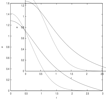
Figure 6:

References

- [1] J.S. Langer, Ann. Phys. 41 (1967) 108.
-
[2]
S. Coleman,
Phys. Rev. D 15 (1977) 2929.
C. Callan and S. Coleman, Phys. Rev. D 16 (1977) 1762. - [3] S. Coleman, V. Glaser and A. Martin, Comm. Math. Phys. 58 (1978) 211.
- [4] A. Linde, Particle Physics and Inflationary Cosmology. Harwood, Chur, Switzerland, 1990.
- [5] G. Mnster and S. Rotsch, Eur. Phys. J. C 12 (2000) 161
-
[6]
Hatem Widyan, A. Mukherjee, N. Panchapakesan and R.P.
Saxena,
Phys. Rev. D 59 (1999) 045003.
Hatem Widyan, A. Mukherjee, N. Panchapakesan and R.P. Saxena, Phys. Rev. D 62 (2000) 025003. - [7] D. Bdeker, L. Fromme, S.J. Huber and M. Seniuch, JHEP 0502 (2005) 026.
- [8] X. Zhang, Phys. Rev. D 47 (1993) 3065
- [9] S.W. Ham and S.K. Oh, Phys.Rev. D 70 (2004) 093007.
- [10] C. Grojean, G. Servant and J.D. Wells, Phys. Rev. D 71 (2005) 036001.
- [11] Yoav Bergner and Luis M. Bettencourt, Phys. Rev. D 68 (2003) 025014.
- [12] M.G. do Amaral, Phys. G 24 (1998) 1061.
- [13] G.H. Flores, R.O. Ramos and N.F. Svaiter, Int. J. Mod. Phys. A 14 (1999) 3715.
- [14] M. Joy and V.C. Kuriakose, Mod. Phys. Lett. A 18 (2003) 937.
- [15] P. Arnold and D. Wright, Phys. Rev. D 55 (1997) 6274.
- [16] A.B. Zamolodchikov, Sov. J. Nucl. Phys. 44 (1986) 529.
- [17] W. Fa Lu, J.G. Ni and Z.G. Wang, J. Phys. G 24 (1998) 673.
- [18] Yoonbai Kim, Kei-ichi Maeda and Nobuyuki Sakai, Nucl.Phys. B 481 (1996) 453.
- [19] Ariel Megevand, Int. J. Mod. Phys. D 9 (2000) 733.
- [20] J. Garriga, Phys. Rev. D 49 (1994) 5497.
- [21] For recent review see Andrei Linde, J. Phys. Conf. Ser. 24 (2005) 151.
-
[22]
S. Digal, S. Sengupta and A.M. Srivastava,
Phys. Rev. D 56 (1997) 2035.
Sang Pyo Kim, Nuovo Cim. B120 (2005) 1209 and more references therein.