Finite Temperature Phase Transition in $\phi^{6}$ potential

Abstract

The temperature dependance of the action in the thin-wall and thick-wall limits is obtained analytically for the $\phi^{6}$ scalar potential. The nature of the phase transition is investigated from the quantum tunnelling regime at low temperatures to the thermal hopping regime at high temperatures. It is first-order for the case of a thin wall while for the thick wall it is second- order.

1. Introduction

The existence of phase transition associated with spontaneous symmetry breaking may appear during the evolution of the the universe. Such a phase transition may influence to the large-scale structure of the universe [1]. Both the order of the phase transition and its strength are basic ingredients for a quantitative discussion of the transition at some energy scale. In general, a symmetry-breaking phase transition can be first or second order one. The decay of metastable state at a given temperature $T$ can be written in the from $\Gamma=A{\rm e}^{-S_{E}(T)}$, with $S_{E}(T)$ being the Euclidean action of the saddle-point configuration and $A$ being the prefactor determined by the associated fluctuations. At zero temperature, the decay is determined by quantum effects. With increasing temperature, the nature of the decay changes from quantum to classical. The function $S_{E}(T)$ might either be a smooth function of temperature or exhibit a kink with a discontinuity in its derivative at some temperature $T_{c}$. In the former case, the transition from the quantum tunneling regime is said to be of second order while in the latter case it is said to be of first order.

We have considered in an earlier work the $\phi^{4}$ theory with different symmetry breaking terms [6, 7], where we have obtained numerical as well as analytical solution for different values of the asymmetric term. In this paper we extend our recent work in $\phi^{6}$ potential [8] which has been investigated by many authors in the context of condensed matter as well as particle physics (see for example [9, 10, 11, 12, 13, 14, 15]). In [8], the scalar potential $\phi^{6}$ is studied at zero temperature and at high temperature. The equations of motion are solved numerically to obtain $O(4)$ spherical symmetric and $O(3)$ cylindrical bounce solutions. Also an analytical solution for the bounce is presented in the thin wall-wall as well as thick-wall limits, where the potential is given by

$$U(\phi)=g\,\phi^{2}(\phi^{2}-\phi_{0}^{2})^{2}-\delta\phi^{2},$$ (1)

where $\phi_{0}^{2}=-\lambda/{2g}$ and $\delta=(\lambda^{2}/g-2m^{2})/4$. Fixing the value of $\phi_{0}=2.39$ and $g=0.07$, the only adjustable parameter in the potential is $\delta$ and its range is $0<\delta<g\phi_{0}^{4}=2.28$. In this paper we extend our calculation of the action in [8] to finite temperatures and study the nature of the transition. We propose a general ansatz at finite temperature in the thin wall ($\delta\rightarrow 0$) and thick wall ($\delta\rightarrow 2.28$) limits. We find that for a thin wall the transition is first-order while for a thick wall it is second-order. In section $2$, we present our analytical calculations of the action at finite temperature in the thin wall limit, while the calculations for the thick wall limit are presented in section $3$. Section $4$ contains our conclusions. The algebraic expressions for integrals appearing in the analytical formalism are given in Appendixes A and B.

2. Action at finite temperature in the thin wall limit

The action at finite temperature of a single scalar field $\phi$ is given by the following formula

$$S(T)=4\pi\int_{-\beta/2}^{\beta/2}d\tau\int_{0}^{\infty}drr^{2}\Bigg{[}\frac{1}{2}\Bigg{(}\frac{\partial\phi}{\partial\tau}\Bigg{)}^{2}+\frac{1}{2}\Bigg{(}\frac{\partial\phi}{\partial r}\Bigg{)}^{2}+U(\phi)\Bigg{]}~{}.$$ (2)

The equation of motion derived from the above action is given by the following expression

$${\partial^{2}\phi\over\partial\tau^{2}}+{\partial^{2}\phi\over\partial r^{2}}+{2\over r}{\partial\phi\over\partial r}={\partial U(\phi,T)\over\partial\phi}~{},$$ (3)

with boundary conditions

$$\phi\to\phi_{-}\quad{\rm as}\quad r\to\infty,\quad\partial\phi/\partial\tau=0\quad{\rm at}\quad\tau=\pm\beta/2,0~{},$$ (4)

where $\phi_{-}$ is the false vacuum of the potential $U$, $\beta$ is the period of the solution and $r=\sqrt{\vec{x}^{2}}.$

Following [8, 9, 11, 12] we assume for the solution of the equation of motion the following ansatz:

$$\phi^{2}(r,\tau)=\frac{\gamma}{e^{{{(r^{2}+\frac{\beta^{2}}{\pi^{2}}{\mathrm{sin}}^{2}(\frac{\pi\tau}{\beta})-R^{2})}/\Lambda^{2}}}+1}~{},$$ (5)

which is periodic in the interval $(-\beta/2,\beta/2)$ and satisfies the required boundary conditions (Eq. (4)), viz

$$\frac{\partial\phi}{\partial r}=0~{}\mathrm{at}~{}r=0,~{}\frac{\partial\phi}{\partial\tau}=0~{}\mathrm{at}~{}\tau=0~{}\mathrm{and}~{}\pm\beta/2,~{}\mathrm{and}~{}\phi=0~{}\mathrm{as}~{}r\to\infty~{}.$$ (6)

We evaluate the action for potential given by Eq. (1)

$$U(\phi)=g\,\phi^{2}(\phi^{2}-\phi_{0}^{2})^{2}-\delta\phi^{2}.$$ (7)

After substituting the ansatz function Eq. (5) into the equation of motion Eq. (3), we have

$$\frac{\sqrt{\gamma}}{(e^{{{(r^{2}+\frac{\beta^{2}}{\pi^{2}}{\mathrm{sin}}^{2}(\frac{\pi\tau}{\beta})-R^{2})}/\Lambda^{2}}}+1)^{5/2}}\Bigg{[}\frac{3r^{2}}{\l^{4}}+\frac{3\beta^{2}}{4\pi^{2}\l^{4}}{\mathrm{sin}}^{2}(\frac{2\pi\tau}{\beta})\Bigg{]}$$

$$+\frac{\sqrt{\gamma}}{(e^{{{(r^{2}+\frac{\beta^{2}}{\pi^{2}}{\mathrm{sin}}^{2}(\frac{\pi\tau}{\beta})-R^{2})}/\Lambda^{2}}}+1)^{3/2}}\Bigg{[}-\frac{4r^{2}}{\l^{4}}+\frac{3}{\l^{2}}+\frac{1}{\l^{2}}{\mathrm{cos}}(\frac{2\pi\tau}{\beta})-\frac{\beta^{2}}{\pi^{2}\l^{4}}{\mathrm{sin}}^{2}(\frac{2\pi\tau}{\beta})\Bigg{]}$$

$$+\frac{\sqrt{\gamma}}{(e^{{{(r^{2}+\frac{\beta^{2}}{\pi^{2}}{\mathrm{sin}}^{2}(\frac{\pi\tau}{\beta})-R^{2})}/\Lambda^{2}}}+1)^{1/2}}\Bigg{[}\frac{r^{2}}{\l^{4}}-\frac{3}{\l^{2}}+\frac{\beta^{2}}{4\pi^{2}\l^{4}}{\mathrm{sin}}^{2}(\frac{2\pi\tau}{\beta})-\frac{1}{\l^{2}}{\mathrm{cos}}(\frac{2\pi\tau}{\beta})\Bigg{]}$$

$$=\frac{6g\gamma^{5/2}}{(e^{{{(r^{2}+\frac{\beta^{2}}{\pi^{2}}{\mathrm{sin}}^{2}(\frac{\pi\tau}{\beta})-R^{2})}/\Lambda^{2}}}+1)^{5/2}}-8g\phi_{0}^{2}\frac{\gamma^{3/2}}{(e^{{{(r^{2}+\frac{\beta^{2}}{\pi^{2}}{\mathrm{sin}}^{2}(\frac{\pi\tau}{\beta})-R^{2})}/\Lambda^{2}}}+1)^{3/2}}$$

$$+2(g\phi_{0}^{4}-\delta)\frac{\gamma^{1/2}}{(e^{{{(r^{2}+\frac{\beta^{2}}{\pi^{2}}{\mathrm{sin}}^{2}(\frac{\pi\tau}{\beta})-R^{2})}/\Lambda^{2}}}+1)^{1/2}}~{}.$$ (8)

In the thin wall limit, the bounce solution is constant except in a narrow region near the wall. Hence, by equating terms with different powers of exponentials separately in Eq. (8), we have with $r^{2}+\frac{\beta^{2}}{4\pi^{2}}{\mathrm{sin}}^{2}(\frac{2\pi\tau}{\beta})\approx R^{2}$,

$$2g\gamma^{2}=\frac{R^{2}}{\l^{4}}\Bigg{[}1-a\frac{\l^{2}}{R^{2}}\Bigg{]}~{}.$$

$$2g\phi_{0}^{2}\gamma=\frac{R^{2}}{\l^{4}}\Bigg{[}1-b\frac{\l^{2}}{R^{2}}\Bigg{]}~{}.$$

$$2(g\phi_{0}^{4}-\delta)=\frac{R^{2}}{\l^{4}}\Bigg{[}1-d\frac{\l^{2}}{R^{2}}\Bigg{]}~{}.$$ (9)

The parameters $a$, $b$ and $d$ are found by the requirement that the variation of $S(T)$ with respect to the parameters $R$, $\l$ and $\gamma$ in Eq. (5) vanishes.

The integrals in the action are obtained in powers of $\l^{2}/R^{2}$ using the usual methods for evaluating integrals of the Fermi function (see eg. Huang [16]). We get

$$S(T) = 4\pi\int_{-\beta/2}^{\beta/2}d\tau\int_{0}^{\infty}drr^{2}\Bigg{[}\frac{1}{2}\Bigg{(}\frac{\partial\phi}{\partial\tau}\Bigg{)}^{2}+\frac{1}{2}\Bigg{(}\frac{\partial\phi}{\partial r}\Bigg{)}^{2}+g\phi^{6}-2g\phi_{0}^{2}\phi^{4}+(g\phi_{0}^{4}-\delta)\phi^{2}\Bigg{]}$$ (10)

$$= 4\pi\kappa R^{4}E_{3}\,\gamma\Bigg{[}\frac{\kappa^{2}}{4\l^{2}}\Bigg{(}\frac{E_{1T}}{E_{3}}+\frac{1}{2}\frac{E_{0T}}{E_{3}}\frac{\l^{2}}{R^{2}}\Bigg{)}+\frac{1}{4\l^{2}}\Bigg{(}1+\frac{3}{2}\frac{E_{1}}{E_{3}}\frac{\l^{2}}{R^{2}}+\frac{\pi^{2}}{8}\frac{E_{0}}{E_{3}}\frac{\l^{4}}{R^{4}}\Bigg{)}$$

$$+ \frac{g\gamma^{2}}{2}\Bigg{(}\frac{4}{3}-\frac{3E_{1}}{E_{3}}\frac{\l^{2}}{R^{2}}+\Big{(}\frac{\pi^{2}}{6}+\frac{1}{2}\Big{)}\frac{E_{0}}{E_{3}}\frac{\l^{4}}{R^{4}}\Bigg{)}$$

$$- 2g\phi_{0}^{2}\gamma\Bigg{(}\frac{2}{3}-\frac{E_{1}}{E_{3}}\frac{\l^{2}}{R^{2}}+\frac{\pi^{2}}{12}\frac{E_{0}}{E_{3}}\frac{\l^{4}}{R^{4}}\Bigg{)}$$

$$+ \frac{1}{2}(g\phi_{0}^{4}-\delta)\Bigg{(}\frac{4}{3}+\frac{\pi^{2}}{6}\frac{E_{0}}{E_{3}}\frac{\l^{4}}{R^{4}}\Bigg{)}\Bigg{]}~{},$$

where

$$E_{0}(\kappa^{2}) = \int_{0}^{1}\frac{dt}{\sqrt{1-t^{2}}\sqrt{1-\kappa^{2}t^{2}}}~{},$$

$$E_{1}(\kappa^{2}) = \int_{0}^{1}\frac{dt\sqrt{1-\kappa^{2}t^{2}}}{\sqrt{1-t^{2}}}~{},$$

$$E_{3}(\kappa^{2}) = \int_{0}^{1}\frac{dt(1-\kappa^{2}t^{2})^{3/2}}{\sqrt{1-t^{2}}}~{},$$

$$E_{0T}(\kappa^{2}) = \int_{0}^{1}\frac{dt(1-t^{2})t^{2}}{\sqrt{1-t^{2}}{\sqrt{1-\kappa^{2}t^{2}}}}~{},$$

$$E_{1T}(\kappa^{2}) = \int_{0}^{1}\frac{dt(1-t^{2})t^{2}\sqrt{1-\kappa^{2}t^{2}}}{\sqrt{1-t^{2}}}~{},$$

are the complete elliptic integrals and they can be represented in terms of the basic complete elliptic integrals $E_{0}$ and $E_{1}$ (see Appendix A), $\kappa=\frac{\beta}{\pi R}$ and $t={\mathrm{sin}}\frac{\pi}{\beta}\tau$.

We now determine the parameters $a$, $b$ and $d$ by demanding the vanishing of $dS(T)/dR^{2}$, $dS(T)/d\l^{2}$ and $dS(T)/d\gamma$. Differentiating Eq. (10) and using Eq. (9), we find that to leading order in $\l^{2}/R^{2}$,

$$-4a+8b-4d+3+\frac{3(E_{1}-2\kappa^{2}E_{1}^{\prime})}{3E_{3}-2\kappa^{2}E_{3}^{\prime}}+\frac{3\kappa^{2}(E_{1T}-2\kappa^{2}E_{1T}^{\prime})}{3E_{3}-2\kappa^{2}E_{3}^{\prime}}=0~{},$$

$$a\Bigg{(}\frac{3}{4}\lambda-\frac{1}{2}g\gamma^{2}\epsilon_{T}\frac{E_{3}}{E_{1}}\Big{(}1-\frac{\lambda}{2g\gamma^{2}}\Big{)}\Bigg{)}+b\Bigg{(}\frac{1}{2}g\gamma^{2}\epsilon_{T}\frac{E_{3}}{E_{1}}-\lambda\Bigg{)}+\frac{1}{4}\frac{E_{0}}{E_{1}}\lambda=0~{},$$

$$-a+\frac{4b}{3}-\frac{1}{3}d-\frac{1}{4}\epsilon_{T}=0~{},$$ (11)

where $\lambda=2g\gamma^{2}-2g\phi_{0}^{2}\gamma$, $E_{1}^{\prime}$ is the derivative of $E_{1}$ with respect to $\kappa^{2}$ (and similarly for $E_{1T}^{\prime}$ and $E_{3}^{\prime}$), and $\epsilon_{T}=E_{1}/E_{3}-\kappa^{2}E_{1T}/E_{3}-1$.

Note that in the limit of zero temperature ($\kappa\rightarrow\infty$), Eq. (11) reduces to

$$3-2a+4b-2d=0,~{}~{}~{}~{}~{}~{}2+3a-4b=0,~{}~{}~{}~{}~{}~{}~{}~{}{\rm and}~{}~{}~{}~{}~{}~{}~{}~{}~{}-3a+4b-d=0,$$

respectively which are obtained earlier [8]. Also, in the limit of high temperature (i.e. $\kappa\rightarrow 0$), they reduce to

$$1-a+2b-d=0,~{}~{}~{}~{}~{}~{}~{}~{}~{}1+3a-4b=0,~{}~{}~{}~{}~{}~{}{\rm and}~{}~{}~{}~{}~{}~{}~{}~{}~{}-3a+4b+d=0,$$

respectively which are also obtained earlier [8].

By using Eq. (11), we can find a relation between the constants $a$, $b$ and $d$,

$$d-a=\frac{3}{4}\epsilon_{T}+\frac{3}{2}+\frac{c}{2}~{},$$

$$d-b=\frac{3}{8}(\epsilon_{T}+c+3)~{},$$

$$b-a=\frac{3}{8}(1+\epsilon_{T})+\frac{c}{8}~{},$$ (12)

where $c$ is given by the following expression

$$c=\frac{3(E_{1}-2\kappa^{2}E_{1}^{\prime})}{3E_{3}-2\kappa^{2}E_{3}^{\prime}}+\frac{3\kappa^{2}(E_{1T}-2\kappa^{2}E_{1T}^{\prime})}{3E_{3}-2\kappa^{2}E_{3}^{\prime}}~{}.$$

Thus Eq. (10) can be expressed in terms of $a$, $b$ and $d$. It reads as

$$S(T) = \frac{2\pi\kappa}{g\phi_{0}^{2}}E_{3}\Bigg{(}\frac{R}{\l}\Bigg{)}^{6}\Bigg{[}\Bigg{(}1-b\frac{\l^{2}}{R^{2}}\Bigg{)}\Bigg{(}\frac{1}{2}\frac{E_{1}}{E_{3}}-\frac{2}{3}(b-a)\Bigg{)}+\frac{E_{1}}{E_{3}}\Bigg{(}\frac{3}{32}\Big{(}2b-d-3-3\epsilon_{T}\Big{)}$$ (13)

$$+ \frac{3}{8}\frac{E_{1}}{E_{3}}+\frac{1}{8}\frac{E_{0}}{E_{3}}+\frac{1}{8}\frac{E_{0T}}{E_{3}}\Bigg{)}\frac{\l^{2}}{R^{2}}\Bigg{]}~{}.$$

With these expressions we can calculate the values of $\gamma$, $R$ and $\l$ and also for the action $S(T)$. In calculating $S(T)$ for $\beta\to\infty$, the integrals $E_{i4}$ are to be used (see Appendix A). In these cases $\kappa>1$ and restrict the upper limit of the elliptic integral to $1/\kappa$ as they become complex for larger values of $\kappa$.

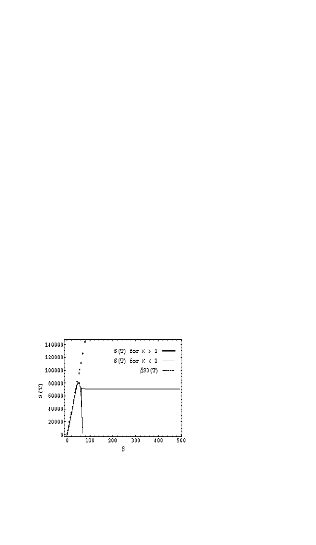
Figure 1: Temperature dependence of the Euclidean actin in thin- wall limit: $S(T)$ vs $\beta$ for $\delta=0.1$

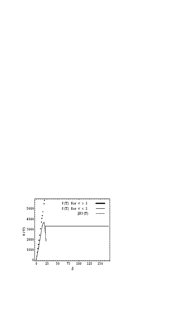
Figure 2: Temperature dependence of the Euclidean actin in thin- wall limit: $S(T)$ vs $\beta$ for $\delta=0.3$

As was noticed in [7], there is a singularity in ($b-a$) due to $E_{0}(\kappa)$ becoming singular at $\kappa=1$. The values of $S(T)$ are obtained and plotted for $\delta=0.1$ and $\delta=0.3$ as shown in Figs. $1$ and $2$ respectively. The inverse of the temperature $\beta_{\star}$ is defined by [6] $\beta_{\star}=S_{4}/S_{3}$. The transition point $\beta_{c}$ can in principle be different from $\beta_{\star}$, but in the TWA are equal [6, 7]. In our results (Figs. 1 and 2) we can determine $\beta_{\star}$ by extending the horizontal part of the curve to the left. For Fig. 1, for example, this yields $\beta_{\star}=$, which is close to the value of $\beta_{c}$ obtained numerically and analytically [7]. We conclude that the singularity is an artifact of the method, and does not represent the transition point. The phase transition actually takes place at a much lower value of $\beta_{c}$, and is first-order.

It can be shown that in the limit of zero temperature ($\kappa\rightarrow\infty$) and in the limit of high temperature ($\kappa\rightarrow 0$), the action in Eq. (13) reduces to the action given earlier [8].

3. Action at finite temperature in the thick wall limit

The form of the bounce in Eq. (5) suggests that the thick wall limit, which would correspond to small values of $R^{2}/\l^{2}$, would be obtained by approximating the Fermi function by the Maxwell-Boltzmann function, which leads to a Gaussian:

$$\phi^{2}(r,\tau)={\gamma}\,{e^{-{{(r^{2}+\frac{\beta^{2}}{\pi^{2}}{\mathrm{sin}}^{2}(\frac{\pi\tau}{\beta}))}/\Lambda^{2}}}}~{},$$ (14)

which satisfies the boundary conditions given by Eq. (6). The action for this form of bounce is found to be

$$S(T) = \frac{\pi}{2}\gamma\Gamma(\frac{3}{2})\l^{4}{\rm e}^{-x^{2}/2}xI_{0}(\frac{x^{2}}{2})\Bigg{[}\frac{3}{4\l^{2}}+\frac{1}{4\l^{2}}\frac{I_{1}(\frac{x^{2}}{2})}{I_{0}(\frac{x^{2}}{2})}-2g\phi_{0}^{2}\gamma(\frac{1}{2})^{3/2}{\rm e}^{-x^{2}/2}\frac{I_{0}(x^{2})}{I_{0}(\frac{x^{2}}{2})}$$ (15)

$$+ g\gamma^{2}(\frac{1}{3})^{3/2}{\rm e}^{-x^{2}}\frac{I_{0}(\frac{3x^{2}}{2})}{I_{0}(\frac{x^{2}}{2})}+(g\phi_{0}^{4}-\delta)\Bigg{]}~{},$$

where $x=\beta/{\pi\l}$ and$I_{\nu}(x^{2})$ are the modified Bessel functions.

Equation (9) then reduces to

$$2g\gamma^{2}=-\frac{a}{\l^{2}},~{}~{}~{}~{}2\phi_{0}^{2}\gamma=-\frac{b}{\l^{2}},~{}~{}~{}~{}2(g\phi_{0}^{4}-\delta)=-\frac{d}{\l^{2}}.$$ (16)

Here we assume $\gamma^{2}<<1$, hence $a=0$. The values of $b$ and $d$ are obtained by demanding $dS(T)/d\gamma=dS(T)/d\l=0$. This gives the following:

$$\frac{3}{4}+\frac{1}{4}\frac{I_{1}(\frac{x^{2}}{2})}{I_{0}(\frac{x^{2}}{2})}+\frac{b}{\sqrt{2}}{\rm e}^{-x^{2}/2}\frac{I_{0}(x^{2})}{I_{0}(\frac{x^{2}}{2})}-\frac{d}{2}=0$$

$$\frac{3}{8}{\rm e}^{-x^{2}/2}\Bigg{(}{I_{0}(\frac{x^{2}}{2})}+{I_{1}(\frac{x^{2}}{2})}\Bigg{)} + \frac{x^{2}}{4}{\rm e}^{-x^{2}/2}\Bigg{(}{I_{0}(\frac{x^{2}}{2})}-{I_{1}(\frac{x^{2}}{2})}\Bigg{)}+b(\frac{1}{2})^{5/2}{\rm e}^{-x^{2}}I_{0}(x^{2})F$$ (17)

$$- \frac{d}{8}{\rm e}^{-x^{2}}{I_{0}(\frac{x^{2}}{2})}E=0$$

where

$$E=6+2x^{2}\Big{(}1-\frac{I_{1}(\frac{x^{2}}{2})}{I_{0}(\frac{x^{2}}{2})}\Big{)}$$

$$F=3+2x^{2}\Big{(}1-\frac{I_{1}(x^{2})}{I_{0}(x^{2})}\Big{)}.$$ (18)

In order to check our results, note that in the limit of zero temperature ($x\rightarrow\infty$), Eqs. (3. Action at finite temperature in the thick wall limit) and (17) reduce to

$$2+b-d=0~{}~{}~{}~{}~{}~{}{\rm and}~{}~{}~{}~{}~{}~{}~{}~{}~{}2+b-2d=0$$

respectively which are obtained earlier [8]. Also, in the limit of high temperature (i.e. $x\rightarrow 0$), they reduce to

$$\frac{3}{16}+\frac{b}{2^{5/2}}-\frac{d}{8}=0~{}~{}~{}~{}~{}~{}{\rm and}~{}~{}~{}~{}~{}~{}~{}~{}~{}\frac{3}{8}+(\frac{1}{2})^{3/2}\frac{3b}{2}-\frac{3d}{4}=0$$

respectively which are obtained earlier [8].

Using the Eqs. (3. Action at finite temperature in the thick wall limit) and (17), the values of $b$ and $d$ are given by

$$b=\frac{\frac{E}{16}\Big{(}3I_{0}(\frac{x^{2}}{2})+I_{1}(\frac{x^{2}}{2})\Big{)}-\frac{3}{8}\Big{(}I_{0}(\frac{x^{2}}{2})+I_{1}(\frac{x^{2}}{2})\Big{)}-\frac{x^{2}}{4}\Big{(}I_{0}(\frac{x^{2}}{2})-I_{1}(\frac{x^{2}}{2})\Big{)}}{(\frac{1}{2})^{5/2}(F-E)I_{0}(x^{2}){\rm e}^{{-x^{2}}/2}}$$ (19)

$$d=\frac{F\Big{(}\frac{3}{2}I_{0}(\frac{x^{2}}{2})+\frac{1}{2}I_{1}(\frac{x^{2}}{2})\Big{)}-3\Big{(}I_{0}(\frac{x^{2}}{2})+I_{1}(\frac{x^{2}}{2})\Big{)}-2x^{2}\Big{(}I_{0}(\frac{x^{2}}{2})-I_{1}(\frac{x^{2}}{2})\Big{)}}{(F-E)I_{0}(\frac{x^{2}}{2})}$$ (20)

In the limit of zero temperature ($x\rightarrow\infty$), $b=-2$ and $d=0$, and in the limit of high temperature ($x\rightarrow 0$), $b=-\sqrt{2}$ and $d=-1/2$, which are the same values obtained earlier [8].

Thus the action yields

$$S(T)=\frac{\pi^{2}}{g\phi_{0}^{2}}b\Gamma(\frac{3}{2})xI_{0}(\frac{x^{2}}{2}){\rm e}^{{-x^{2}}/2}\Big{(}\frac{3}{4}+\frac{1}{4}\frac{I_{1}(\frac{x^{2}}{2})}{I_{0}(\frac{x^{2}}{2})}\Big{)}+b(\frac{1}{2})^{3/2}{\rm e}^{{-x^{2}}/2}\frac{I_{0}(x^{2})}{I_{0}(\frac{x^{2}}{2})}-\frac{d}{2}.$$ (21)

It can be shown that in the limit of zero temperature ($x\rightarrow\infty$) and in the limit of high temperature ($x\rightarrow 0$), the action obtained the the last equation reduces to the action given earlier [8].

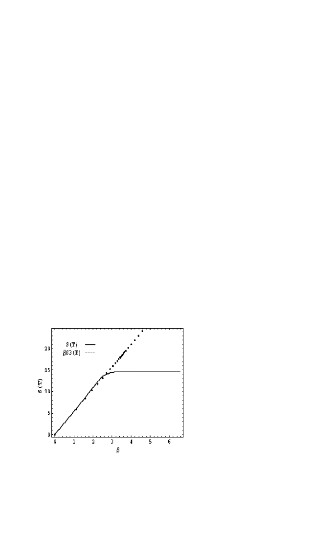
Figure 3: Temperature dependence of the Euclidean actin in thick- wall limit: $S(T)$ vs $\beta$ for $\delta=2.0$

For a given value of temperature (i.e. $x$), we can calculate $b$ and $d$. Here, $\gamma$ and $\Lambda$ are determined. Thus we can calculate the action at different values of temperatures. Fig. 3 shows the value of the action at different values of inverse of temperature for $\delta=2.0$. As we can see from the figure, the action goes smoothly from the zero temperature regime to the high temperature regime without any singularity at the transition point. This means that in the thick-wall limit the transition is second order. Moreover, the action at zero temperature is independent of the value of $\delta$ as shown in our earlier work [8], which has been also verified in our calculations here.

4. Conclusions

We now discuss the nature of the transition as we go from zero to high temperatures. In quantum mechanics, definitive criteria for the continuity or discontinuity (corresponding to second order and first order respectively) in the derivative of the action have been obtained by Chudnovsky [17] and Garriga [18]. It has even been shown that the lowest action at any temperature is possessed by either the zero temperature or the high temperature solutions.

In quantum field theory the situation seems to be different. Both Ferrera [19] and we [6] find that there is an interpolating solution which can be used to determine whether transition is first order or second order (i.e. with or without a kink).

We have found that for a thin wall ($\delta\rightarrow 0$) the interpolating solution has a singularity at $\beta=\pi R$. But it is not a real singularity at this point. It is due to the expansion method used in the calculations. Our numerical solutions show a kink is present in the TWA, showing that the transition is first order. However, for $\delta=2$ (thick wall), we find there is no kink and the transition is smooth (second order).

We would to mention here that the Eqs. (5) and (14) are not an exact solutions of the equations of motion at finite temperature although they satisfy the required boundary conditions. We think they represent a reasonable approximation because in the case of thin wall approximation at zero temperature Eq. (5) is a solution of the equation of the motion, see [11].

It is suggested that our method could be used to study in detail the nature of the phase transition in electroweak theory. Such a study could be of importance in models of electroweak baryogenesis and other phenomena in the early universe.

Appendix A EXPRESSIONS OF ELLIPTIC INTEGRAL IN TERMS OF THE BASIC INTEGRALS $E_{0}$ AND $E_{1}$

For $\kappa<1$

$$E_{0} = \int_{0}^{1}\frac{dt}{\sqrt{1-t^{2}}\sqrt{1-\kappa^{2}t^{2}}}$$ (22)

$$E_{1} = \int_{0}^{1}\frac{dt\sqrt{1-\kappa^{2}t^{2}}}{\sqrt{1-t^{2}}}$$ (23)

$$E_{3} = \int_{0}^{1}\frac{dt(1-\kappa^{2}t^{2})^{3/2}}{\sqrt{1-t^{2}}}=E_{1}(\frac{4}{3}-\frac{2}{3}\kappa^{2})+E_{0}(\frac{\kappa^{2}-1}{3})$$ (24)

$$E_{0T} = \int_{0}^{1}\frac{dt(1-t^{2})t^{2}}{\sqrt{1-t^{2}}\sqrt{1-\kappa^{2}}}=E_{1}(\frac{2}{3}\frac{1}{\kappa^{4}}-\frac{1}{3}\frac{1}{\kappa^{2}}+E_{0}(\frac{2}{3}\frac{1}{\kappa^{2}}-\frac{2}{3}\frac{1}{\kappa^{2}})$$ (25)

$$E_{1T} = \int_{0}^{1}\frac{dt\sqrt{1-\kappa^{2}t^{2}}t^{2}(1-t^{2})}{\sqrt{1-t^{2}}}=\frac{2E_{1}}{15}(\frac{1}{\kappa^{4}}-\frac{1}{\kappa^{2}}+1)+\frac{E_{0}}{15}(-\frac{2}{\kappa^{4}}+\frac{3}{\kappa^{2}}-1)$$ (26)

$$E_{1}^{\prime} = \frac{E_{1}-E_{0}}{2\kappa^{2}}$$ (27)

$$E_{3}^{\prime} = \frac{E_{0}}{2}(1-\frac{1}{\kappa^{2}})+E_{1}(-1+\frac{1}{2\kappa^{2}})$$ (28)

$$E_{1T}^{\prime} = \frac{E_{1}}{15}(-\frac{4}{\kappa^{6}}+\frac{3}{2\kappa^{4}}+\frac{1}{\kappa^{2}})+\frac{E_{0}}{15}(\frac{4}{\kappa^{6}}-\frac{7}{2\kappa^{4}}-\frac{1}{2\kappa^{2}})$$ (29)

For $\kappa>1$

$$E_{0}(1/\kappa^{2}) = \int_{0}^{1}\frac{dt}{\sqrt{1-t^{2}}\sqrt{1-t^{2}/\kappa^{2}}}$$ (30)

$$E_{1}(1/\kappa^{2}) = \int_{0}^{1}\frac{dt\sqrt{1-t^{2}/\kappa^{2}}}{\sqrt{1-t^{2}}}$$ (31)

$$E_{04}(\kappa^{2}) = \int_{0}^{1/\kappa}\frac{dt}{\sqrt{1-t^{2}}\sqrt{1-\kappa^{2}t^{2}}}$$ (32)

$$E_{14}(\kappa^{2}) = \int_{0}^{1/\kappa}\frac{dt\sqrt{1-\kappa^{2}t^{2}}}{\sqrt{1-t^{2}}}=\kappa E_{1}(1/\kappa^{2})-\frac{\kappa^{2}-1}{\kappa}E_{0}(1/\kappa^{2})$$ (33)

$$E_{34}(\kappa^{2}) = \int_{0}^{1/\kappa}\frac{dt(1-\kappa^{2}t^{2})^{3/2}}{\sqrt{1-t^{2}}}=\frac{1}{\kappa}\Bigg{[}E_{1}(1/\kappa^{2})\Big{(}\frac{4\kappa^{2}}{3}-\frac{2\kappa^{4}}{3}\Big{)}$$ (34)

$$+ E_{0}(1/\kappa^{2})\Big{(}1-\frac{5\kappa^{2}}{3}+\frac{2\kappa^{4}}{3}\Big{)}\Bigg{]}$$

$$E_{0T4}(\kappa^{2}) = \int_{0}^{1/\kappa}\frac{dt\sqrt{1-\kappa^{2}t^{2}}t^{2}}{(1-t^{2})\sqrt{1-t^{2}}}=\frac{1}{\kappa}\Bigg{[}E_{1}(1/\kappa^{2})\Big{(}-\frac{1}{3}+\frac{2}{3\kappa^{2}}\Big{)}$$ (35)

$$+ E_{0}(1/\kappa^{2})\Big{(}\frac{1}{3}-\frac{1}{3\kappa^{2}}\Big{)}\Bigg{]}$$

$$E_{1T4}(\kappa^{2}) = \int_{0}^{1/\kappa}\frac{dt\sqrt{1-\kappa^{2}t^{2}}t^{2}(1-t^{2})}{\sqrt{1-t^{2}}}=\frac{1}{\kappa}\Bigg{[}E_{1}(1/\kappa^{2})\Big{(}-\frac{2}{15}+\frac{2}{15\kappa^{2}}+\frac{2\kappa^{2}}{15}\Big{)}$$ (36)

$$+ E_{0}(1/\kappa^{2})\Big{(}\frac{1}{5}-\frac{1}{15\kappa^{2}}-\frac{2\kappa^{2}}{15}\Big{)}\Bigg{]}$$

$$\frac{dE_{0}(1/\kappa^{2})}{d\kappa^{2}} = \frac{1}{2\kappa^{2}}E_{0}(1/\kappa^{2})-\frac{E_{1}(1/\kappa^{2})}{2(\kappa^{2}-1)}$$ (37)

$$\frac{dE_{1}(1/\kappa^{2})}{d\kappa^{2}} = \frac{1}{2\kappa^{2}}\Bigg{(}E_{0}(1/\kappa^{2})-E_{1}(1/\kappa^{2})\Bigg{)}$$ (38)

$$\frac{dE_{14}(\kappa^{2})}{d\kappa^{2}} = \frac{1}{2\kappa}\Bigg{(}E_{1}(1/\kappa^{2})-E_{0}(1/\kappa^{2})\Bigg{)}$$ (39)

$$\frac{dE_{34}(\kappa^{2})}{d\kappa^{2}} = E_{(}1/\kappa^{2})\Bigg{(}\frac{1}{2\kappa}-\kappa\Bigg{)}+E_{0}(1/\kappa^{2})\Bigg{(}-\frac{1}{\kappa}+k\Bigg{)}$$ (40)

$$\frac{dE_{0T4}(\kappa^{2})}{d\kappa^{2}} = E_{0}(1/\kappa^{2})\Bigg{(}-\frac{1}{6\kappa^{3}}+\frac{2}{3\kappa^{5}}\Bigg{)}+E_{1}(1/\kappa^{2})\Bigg{(}\frac{1}{6\kappa^{3}}-\frac{4}{3\kappa^{5}}\Bigg{)}$$ (41)

$$\frac{dE_{1T4}(\kappa^{2})}{d\kappa^{2}} = E_{0}(1/\kappa^{2})\Bigg{(}\frac{2}{15\kappa^{5}}-\frac{1}{15\kappa^{3}}-\frac{1}{15\kappa}\Bigg{)}+E_{1}(1/\kappa^{2})\Bigg{(}-\frac{4}{15\kappa^{5}}+\frac{1}{10\kappa^{3}}+\frac{1}{15\kappa}\Bigg{)}$$ (42)