Supersymmetric partners for the
associated Lamé potentials

Abstract

The general solution of the stationary Schrödinger equation for the associated Lamé potentials with an arbitrary real energy is found. The supersymmetric partners are generated by employing seeds solutions for factorization energies inside the gaps.

I Introduction

In quantum mechanics the exactly solvable models (ESM) are essential: since the complete physical information is encoded in few analytic expressions, they are ideal to test the convergence of numerical methods. Moreover, the ESM constitute the starting point for applying perturbation techniques. There are some other models, intermediate between the exactly solvable ones and those which can be solved just numerically, which are known nowadays as quasi-exactly solvable (QES). For them there exist analytical expressions encoding just partial physical information, e.g., for only a part of the Hamiltonian spectrum us94 . Along the years several systems have been identified as belonging to the QES class, in particular, there was a dominant conviction that the associated Lamé potentials were QES rkp05 . However, very recently it was shown that the associated Lamé potentials for $(m,\ell)$ integers are exactly solvable, in the sense that the stationary Schrödinger equation admits analytic solutions for any value of the energy parameter fg05 ; fg07 . The initial motivation to look for this result was the need to implement supersymmetric quantum mechanics for generating new exactly solvable models (periodic and asymptotically periodic) df98 ; ks99 ; fnn00 ; fmrs02a ; fmrs02b ; sgnn03 . In order to implement non-singular transformations of general type, the explicit expressions for the Schrödinger solutions in the gaps as well as the band edge eigenfunctions were required fmrs02a ; fmrs02b .

In the next section we will discuss two techniques to find the general solution for the associated Lamé equation for an arbitrary value of the energy parameter: first an ansatz based procedure and then a systematic technique related to the well known Frobenius method. In section 3 we will apply the supersymmetry transformations for generating new periodic and asymptotically periodic potentials which are almost isospectral to the initial associated Lamé potential. In section 4 our general results will be illustrated through the particular case characterized by $(m,\ell)=(3,2)$. Our conclusions will be finally given at section 5.

II General solutions of the associated Lamé equation

We want to find the general solution of the Schrödinger equation for the associated Lamé potentials with an arbitrary value of the energy parameter $E$:

$$H\psi(x)=\left[-\partial^{2}_{x}+V(x)\right]\psi(x)=E\psi(x),$$ (1)

$$V(x)=m(m+1)k^{2}{\rm sn}^{2}x+\ell(\ell+1)k^{2}\frac{{\rm cn}^{2}x}{{\rm dn}^{2}x},$$ (2)

where $m,\ell\in{\mathbb{N}},\ m\geq\ell$, and ${\rm sn}x\equiv{\rm sn}(x,k)$, ${\rm cn}x\equiv{\rm cn}(x,k)$, ${\rm dn}x\equiv{\rm dn}(x,k)$ are the Jacobi elliptic functions of real periods $4K,\ 4K$ and $2K$ respectively fg05 ; fg07 . This is the associated Lamé equation, which can be also expressed in Weierstrass form:

$$-\frac{d^{2}\psi}{dz^{2}}+\left[m(m+1)\wp(z)+\frac{\ell(\ell+1)\bar{e}_{2}\bar{e}_{3}}{\wp(z)-e_{1}}\right]\psi=\widetilde{E}\psi,$$ (3)

through the changes

$$z=\frac{x-iK^{\prime}}{\sqrt{\bar{e}_{3}}},\quad\bar{e}_{i}=e_{1}-e_{i},\quad i=2,3,\quad\widetilde{E}=e_{3}m(m+1)+[E-\ell(\ell+1)]\bar{e}_{3},$$

$\wp(z)\equiv\wp(z,\omega,\omega^{\prime})$ being the Weierstrass elliptic function of half-periods $\omega=K/\sqrt{\bar{e}_{3}}$, $\omega^{\prime}=iK^{\prime}/\sqrt{\bar{e}_{3}}$.

In order to solve (3), let us denote by $\psi^{\pm}(z)$ two linearly independent solutions. Thus, their product $\Psi(z)=\psi^{+}\psi^{-}$ will satisfy the following third-order equation:

$$\frac{d^{3}\Psi}{dz^{3}}-4\left[m(m+1)\wp(z)+\frac{\ell(\ell+1)\bar{e}_{2}\bar{e}_{3}}{\wp(z)-e_{1}}-\widetilde{E}\right]\frac{d\Psi}{dz}$$

$$-2\left\{m(m+1)-\frac{\ell(\ell+1)\bar{e}_{2}\bar{e}_{3}}{[\wp(z)-e_{1}]^{2}}\right\}\wp^{\prime}(z)\Psi=0.$$ (4)

In the first place let us consider the following ansatz for $\Psi$:

$$\Psi(z)=[\wp(z)-e_{1}]+A_{1}+\frac{A_{2}}{\wp(z)-e_{1}}.$$ (5)

By plugging this in equation (4), the parameters $A_{1},\ A_{2},\ \ell,m$ can be fitted fg05 :

$$(a)\quad m=1,\quad\ell=1, \quad A_{1}=\widetilde{E}+e_{1}, \quad A_{2}=\bar{e}_{2}\bar{e}_{3},$$

$$(b)\quad m=1,\quad\ell=0, \quad A_{1}=\widetilde{E}+e_{1}, \quad A_{2}=0.$$

Once $\Psi(z)$ has been gotten, it is straightforward to find $\psi^{\pm}(z)$ through the formula:

$$\psi^{\pm}(z)=\sqrt{\Psi(z)}\exp\left(\mp\frac{1}{2}\int^{z}\frac{d\tau}{\Psi(\tau)}\right).$$ (6)

In the non-trivial case (a) with $(m,\ell)=(1,1)$, in which the associated Lamé equation is not directly the Lamé one, the corresponding solution reads:

$$\psi_{\pm}(x) = \frac{\prod\limits^{2}_{r=1}\sigma\left(\frac{x-iK^{\prime}}{\sqrt{\bar{e}_{3}}}\pm a_{r}\right)}{\sigma\left(\frac{x-iK^{\prime}}{\sqrt{\bar{e}_{3}}}+\omega_{1}\right)\sigma\left(\frac{x-iK^{\prime}}{\sqrt{\bar{e}_{3}}}\right)}\exp\left[\mp\frac{x}{\sqrt{\bar{e}_{3}}}\sum\limits^{2}_{r=0}\zeta(a_{r})\right],$$

where $\omega_{1}=\omega$, $\zeta^{\prime}(z)=-\wp(z),\ [\ln\sigma(z)]^{\prime}=\zeta(z)$.

On the other hand, for a modified ansatz of kind fg05 :

$$\Psi(z)=[\wp(z)-e_{1}]^{2}+B_{1}[\wp(z)-e_{1}]+B_{2}+\frac{B_{3}}{\wp(z)-e_{1}},$$

it turns out that

$$(c)\>m=2,\quad\ell=1, B_{1}=2e_{1}+\frac{\widetilde{E}}{3},\quad B_{2}=\left(\frac{\widetilde{E}}{3}-e_{1}\right)B_{1},\quad B_{3}=\frac{\bar{e}_{2}\bar{e}_{3}B_{1}}{3},$$

$$(d)\>m=2,\quad\ell=0, B_{1}=2e_{1}+\frac{\widetilde{E}}{3},\quad B_{2}=\left(\frac{\widetilde{E}}{3}-e_{1}\right)B_{1}+\bar{e}_{2}\bar{e}_{3},\quad B_{3}=0.$$

Once again, in the case (c) with $(m,\ell)=(2,1)$, in which the associated Lamé equation is not the Lamé one, the corresponding $\psi$ solutions are:

$$\psi_{\pm}(x) = \frac{\prod\limits^{3}_{r=1}\sigma\left(\frac{x-iK^{\prime}}{\sqrt{\bar{e}_{3}}}\pm b_{r}\right)}{\sigma\left(\frac{x-iK^{\prime}}{\sqrt{\bar{e}_{3}}}+\omega_{1}\right)\sigma^{2}\left(\frac{x-iK^{\prime}}{\sqrt{\bar{e}_{3}}}\right)}\exp\left[\mp\frac{x}{\sqrt{\bar{e}_{3}}}\sum\limits^{3}_{r=0}\zeta(b_{r})\right].$$

Although the previous approach allows to find the solutions of equations (3-4) for some integer values of the parameters $(m,\ell)$, however it is not completely systematic. In order to fill the gap, let us use the Frobenius method for solving (4) fg07 . With this aim, let us make the following changes:

$$y=\frac{e_{1}-\wp(z)}{\bar{e}_{2}},\qquad\Phi(y)=[\wp(z)-e_{1}]^{\ell}\Psi.$$ (7)

Therefore, the following equation for $\Phi$ is obtained:

$$P_{4}(y)\frac{d^{3}\Phi}{dy^{3}}+P_{3}(y)\frac{d^{2}\Phi}{dy^{2}}+P_{2}(y)\frac{d\Phi}{dy}+P_{1}(y)\Phi=0,$$ (8)

where $P_{i}(y)$ are the following $i$-th degree polynomials in $y$:

$$\hskip-14.22636ptP_{4}(y)\!=2y^{2}(\bar{e}_{2}y^{2}-\!3e_{1}y+\bar{e}_{3}),\quad P_{3}(y)\!=3y[\bar{e}_{2}(3\!-\!2\ell)y^{2}\!-\!6e_{1}(1\!-\!\ell)y+\!\bar{e}_{3}(1\!-\!2\ell)],$$

$$\hskip-14.22636ptP_{2}(y)=2\{\bar{e}_{2}(3\ell^{2}-m^{2}-6\ell-m+3)y^{2}-[\widetilde{E}+e_{1}(9\ell^{2}-m^{2}-9\ell-m+3)]y+\ell(2\ell-1)\bar{e}_{3}\},$$

$$\hskip-14.22636ptP_{1}(y)=\bar{e}_{2}(2\ell-1)(m+\ell)(m-\ell+1)y+2\ell[\widetilde{E}+e_{1}(3\ell^{2}-m^{2}-m)].$$

Let us propose now

$$\Phi=\sum\limits_{r=0}^{\infty}a_{r}y^{r+\rho},$$ (9)

from which the next equations arise

$$a_{0}f_{0}(\rho)=0,\quad a_{1}f_{0}(\rho+1)+a_{0}f_{1}(\rho)=0,$$

$$\hskip-14.22636pta_{r+2}f_{0}(\rho+r+2)+a_{r+1}f_{1}(\rho+r+1)+a_{r}f_{2}(\rho+r)=0,$$

$$f_{0}(\rho)=\bar{e}_{3}\rho(\rho-1-2\ell)(2\rho-2\ell-1),\quad f_{1}(\rho)=2(\rho-\ell)\{e_{1}[m(m+1)-3(\rho-\ell)^{2}]-\widetilde{E}\},$$

$$f_{2}(\rho)=\bar{e}_{2}(\rho-m-\ell)(\rho+m-\ell+1)(2\rho+1-2\ell).$$

From the three roots $\rho=0,\ \rho=2\ell+1,\ \rho=\ell+1/2$ of the indicial equation $f_{0}(\rho)=0$, the series (9) can be made finite just for $\rho=0$, since for $r=2\ell-1$ it turns out that

$$a_{2\ell}f_{1}(2\ell)+a_{2\ell-1}f_{2}(2\ell-1)=0\quad\Rightarrow\quad a_{r}=\frac{(-1)^{r}F_{r}}{\prod\limits^{r}_{s=1}f_{0}(s)}a_{0}\,,\quad r=1,2,\dots,2\ell,$$ (10)

where the determinant family

$$F_{r}\!=\!\left|\begin{array}[]{llllll}f_{1}(r-1)&f_{2}(r-2)&\hskip 19.91684pt0&\hskip 19.91684pt0&\cdots&\hskip 8.5359pt0\\ f_{0}(r-1)&f_{1}(r-2)&f_{2}(r-3)&\hskip 19.91684pt0&\cdots&\hskip 8.5359pt0\\ \hskip 19.91684pt0&f_{0}(r-2)&f_{1}(r-3)&f_{2}(r-4)&\cdots&\hskip 8.5359pt0\\ \hskip 11.38092pt\cdots&\hskip 11.38092pt\cdots&\hskip 11.38092pt\cdots&\hskip 11.38092pt\cdots&\cdots&\cdots\\ \hskip 19.91684pt0&\hskip 19.91684pt0&\hskip 19.91684pt0&\hskip 19.91684pt0&\cdots&f_{1}(0)\\ \end{array}\right|,$$ (16)

satisfies the following recurrence relationship:

$$F_{r}=f_{1}(r-1)F_{r-1}-f_{2}(r-2)f_{0}(r-1)F_{r-2},\quad r\in{\mathbb{N}},\quad F_{0}\equiv 1,\quad F_{-1}\equiv 0.$$ (17)

In addition, we have to fix $a_{2\ell+1}$ so that the series ends up after $(N+1)$ terms, i.e.,

$$a_{N}f_{1}(N)+a_{N-1}f_{2}(N-1)=0,\quad a_{N+1}=0,\quad f_{2}(N)=0.$$

The previous equations imply that

$$N=m+\ell,\quad a_{m+\ell}f_{1}(m+\ell)+a_{m+\ell-1}f_{2}(m+\ell-1)=0,\quad a_{m+\ell+1}=0.$$

Two different cases can be identified:

(i) For $m=\ell$ it turns out that formula (10) provides all non-null $a_{r}$, $r=0,1,\dots,2\ell$.

(ii) For $m=\ell+\nu,\>\nu=1,2,\ldots$, equation (10) supplies just $a_{r},\ r=1,\dots,2\ell$, while the remaining non-null coefficients are given by:

$$a_{2\ell+r}=\frac{(-1)^{r}D_{\nu-r}\prod\limits_{s=0}^{r-1}f_{2}(2\ell+s)}{D_{\nu}}a_{2\ell},\quad r=1,2,\ldots\nu,$$ (18)

where $D_{r}$ is the minor of $F_{2\ell+\nu+1-r}$ in Laplace expansion of the determinant $F_{2\ell+\nu+1}$.

By coming back now to equation (7), up to a constant factor in both cases we have

$$\Psi(z)=\frac{\prod\limits_{r=1}^{m+\ell}\left[\wp(z)-\wp(b_{r})\right]}{[\wp(z)-e_{1}]^{\ell}},$$

$\wp(b_{1}),\wp(b_{2}),\ldots,\wp(b_{m+\ell})$ being the zeros of $\sum\limits_{r=0}^{m+\ell}a_{r}[(e_{1}-t)/\bar{e}_{2}]^{r}$. By using once again equation (6), the solutions of the associated Lamé equation are finally:

$$\hskip-14.22636pt\psi^{\pm}(x)\!=\!\frac{\prod\limits_{r=1}^{m+\ell}\sigma(\frac{x-iK^{\prime}}{\sqrt{\bar{e}_{3}}}\pm b_{r})}{\sigma^{\ell}(\frac{x-iK^{\prime}}{\sqrt{\bar{e}_{3}}}+\omega_{1})\sigma^{m}(\frac{x-iK^{\prime}}{\sqrt{\bar{e}_{3}}})}\exp\left\{\frac{x}{\sqrt{\bar{e}_{3}}}\left[\ell\zeta(\omega_{1})\mp\sum\limits_{r=1}^{m+\ell}\zeta(b_{r})\right]\right\}.$$ (19)

Note that the well known solutions of the Lamé equation are recovered for $\ell=0$:

$$\psi^{\pm}(x)=\frac{\prod\limits_{r=1}^{m}\sigma(\frac{x-iK^{\prime}}{\sqrt{\bar{e}_{3}}}\pm b_{r})}{\sigma^{m}(\frac{x-iK^{\prime}}{\sqrt{\bar{e}_{3}}})}\exp\left[\mp\frac{x}{\sqrt{\bar{e}_{3}}}\sum\limits_{r=1}^{m}\zeta(b_{r})\right].$$

III Supersymmetry transformations

The supersymmetric quantum mechanics, as an approach to generate new exactly solvable Hamiltonians $\widetilde{H}$ from an initial solvable one $H$, is based on the intertwining relation

$$\widetilde{H}B=BH.$$ (20)

This means that the eigenfunctions of $\widetilde{H}$ are constructed through the non-null action of $B$ onto the eigenfunctions of $H$. If $B$ is a $k$-th order differential operator it turns out that ais93 ; aicd95

$$\widetilde{V}(x)=V(x)-2[\ln W(u_{1},\dots,u_{k})]^{\prime\prime},$$ (21)

where $u_{i}$ are solutions, which can be nonphysical, of the stationary Schrödinger equation associated to $k$ different factorization energies $\epsilon_{i},i=1,\dots,k$, i.e.

$$Hu_{i}=\epsilon_{i}u_{i}.$$ (22)

For periodic potentials, it has been realized that when Bloch-type seed solutions associated to factorization energies which belong to the energy gaps are used, then the SUSY partner potentials $\widetilde{V}(x)$ are again periodic, isospectral to the initial one fnn00 ; fmrs02a ; fmrs02b . On the other hand, when appropriate linear combinations of the solutions (19) are employed, the SUSY partner potentials $\widetilde{V}(x)$ of $V(x)$ become asymptotically periodic, with periodicity defects appearing due to the creation for $\widetilde{H}$ of bound states embedded into the gaps fmrs02a ; fmrs02b . This suggests a natural ordering for the SUSY transformations of periodic potentials which will be next followed (we restrict ourselves to first and second-order techniques).

III.1 Periodic first-order SUSY partner potentials

Let us take $u(x)=\psi^{\pm}(x)$ (see (19)) with $\epsilon<E_{0}$, where $E_{0}$ is the lowest band edge eigenvalue for the corresponding associated Lamé potential. The periodic first-order SUSY partner potentials of $V(x)$ thus read

$$\widetilde{V}_{\pm}(x) = m(m-1)k^{2}{\rm sn}^{2}x+\ell(\ell-1)k^{2}\frac{{\rm cn}^{2}x}{{\rm dn}^{2}x}+2k^{2}\sum\limits_{r=1}^{m+\ell}{\rm sn}^{2}(x\pm\sqrt{\bar{e}_{3}}b_{r}).$$ (23)

III.2 Asymptotically periodic first-order SUSY partner potentials

Let us choose now $u(x)$ as a general linear combination of the solutions $\psi^{\pm}$ ($\epsilon<E_{0}$),

$$\hskip-5.0ptu(x)=A\psi^{+}(x)+B\psi^{-}(x)=A\psi^{+}(x)\phi_{+}(x)=B\psi^{-}(x)\phi_{-}(x),$$ (24)

$$\hskip-10.0pt\phi_{\pm}(x)\!=\!1+\lambda_{\pm}\frac{\psi_{\mp}(x)}{\psi_{\pm}(x)}\!=\!1+\lambda_{\pm}\prod\limits_{r=1}^{m+\ell}\frac{\sigma(\frac{x-iK^{\prime}}{\sqrt{\bar{e}_{3}}}\mp b_{r})e^{\pm 2x\zeta(b_{r})/\sqrt{\bar{e}_{3}}}}{\sigma(\frac{x-iK^{\prime}}{\sqrt{\bar{e}_{3}}}\pm b_{r})},\ \lambda_{+}=\frac{B}{A},\ \lambda_{-}=\frac{A}{B}.$$ (25)

The first-order SUSY partners for the associated Lamé potentials become now asymptotically periodic, with explicit expressions given by

$$\widetilde{V}^{np}(x)=\widetilde{V}_{\pm}(x)-2[\ln\phi_{\pm}(x)]^{\prime\prime},$$ (26)

where $\widetilde{V}_{\pm}(x)$ is given by (23). The spectrum of the Hamiltonian $\widetilde{H}^{np}$ contains the allowed energy bands of $H$ but in addition it has an isolated bound state at $E=\epsilon$.

III.3 Periodic second-order SUSY partner potentials

Let us take now two factorization energies $\epsilon_{1,2}$ inside the same energy gap, and the corresponding Schrödinger seed solutions in the way

$$u_{1}(x)=\psi_{1}^{+}(x)=\frac{\prod\limits_{r=1}^{m+\ell}\sigma(\frac{x-iK^{\prime}}{\sqrt{\bar{e}_{3}}}+b_{r})}{\sigma^{\ell}(\frac{x-iK^{\prime}}{\sqrt{\bar{e}_{3}}}+\omega_{1})\sigma^{m}(\frac{x-iK^{\prime}}{\sqrt{\bar{e}_{3}}})}\exp\left\{{\frac{x}{\sqrt{\bar{e}_{3}}}\left[\ell\zeta(\omega_{1})-\sum\limits_{r=1}^{m+\ell}\zeta(b_{r})\right]}\right\},$$

$$u_{2}(x)=\psi_{2}^{+}(x)=\frac{\prod\limits_{r=1}^{m+\ell}\sigma(\frac{x-iK^{\prime}}{\sqrt{\bar{e}_{3}}}+b^{\prime}_{r})}{\sigma^{\ell}(\frac{x-iK^{\prime}}{\sqrt{\bar{e}_{3}}}+\omega_{1})\sigma^{m}(\frac{x-iK^{\prime}}{\sqrt{\bar{e}_{3}}})}\exp\left\{{\frac{x}{\sqrt{\bar{e}_{3}}}\big{[}\ell\zeta(\omega_{1})-\sum\limits_{r=1}^{m+\ell}\zeta(b^{\prime}_{r})\big{]}}\right\}.$$

It turns out that the Wronskian of $u_{1,2}$ is nodeless, which is conveniently expressed as:

$$W(u_{1},u_{2})=\psi_{1}^{+}(x)\,\psi_{2}^{+}(x)\,g(x)\quad g(x)=\left[\ln\left(\frac{\psi_{2}^{+}}{\psi_{1}^{+}}\right)\right]^{\prime}.$$

The second-order SUSY partner potentials of $V(x)$ become periodic:

$$\hskip-85.35826pt\widetilde{V}(x)=m(m-3)k^{2}{\rm sn}^{2}x+\ell(\ell-3)k^{2}\frac{{\rm cn}^{2}x}{{\rm dn}^{2}x}$$

$$\hskip 85.35826pt+2k^{2}\sum\limits_{r=1}^{m+\ell}\left[{\rm sn}^{2}(x+\sqrt{\bar{e}_{3}}b_{r})+{\rm sn}^{2}(x+\sqrt{\bar{e}_{3}}b^{\prime}_{r})\right]-2\left(\ln g\right)^{\prime\prime}.$$ (27)

III.4 Asymptotically periodic second-order SUSY partner potentials

Let us choose once again $\epsilon_{1,2}$ in the same energy gap but now $u_{1,2}$ are general linear combinations of $\psi^{\pm}$,

$$u_{1}(x)=\psi_{1}^{+}+\lambda_{1}^{+}\psi_{1}^{-}=\psi_{1}^{+}\phi_{1}^{+},\quad u_{2}(x)=\psi_{2}^{+}+\lambda_{2}^{+}\psi_{2}^{-}=\psi_{2}^{+}\phi_{2}^{+},$$ (28)

where

$$\phi_{1}^{+}=1+\lambda_{1}^{+}\frac{\psi_{1}^{-}}{\psi_{1}^{+}}=1+\lambda_{1}^{+}\prod\limits_{r=1}^{m+\ell}\frac{\sigma(\frac{x-iK^{\prime}}{\sqrt{\bar{e}_{3}}}-b_{r})e^{2x\zeta(b_{r})/\sqrt{\bar{e}_{3}}}}{\sigma(\frac{x-iK^{\prime}}{\sqrt{\bar{e}_{3}}}+b_{r})},$$ (29)

$$\phi_{2}^{+}=1+\lambda_{2}^{+}\frac{\psi_{2}^{-}}{\psi_{2}^{+}}=1+\lambda_{2}^{+}\prod\limits_{r=1}^{m+\ell}\frac{\sigma(\frac{x-iK^{\prime}}{\sqrt{\bar{e}_{3}}}-b^{\prime}_{r})e^{2x\zeta(b^{\prime}_{r})/\sqrt{\bar{e}_{3}}}}{\sigma(\frac{x-iK^{\prime}}{\sqrt{\bar{e}_{3}}}+b^{\prime}_{r})}.$$ (30)

An appropriate choice of $\lambda_{1,2}^{+}$ leads to a nodeless Wronskian, which is expressed as:

$$W(u_{1},u_{2})=u_{1}u_{2}g^{np}=\psi_{1}^{+}\psi_{2}^{+}\phi_{1}^{+}\phi_{2}^{+}g^{np},$$

$$g^{np}=\left[\ln\left(\frac{u_{2}}{u_{1}}\right)\right]^{\prime}=\left[\ln\left(\frac{\psi_{2}^{+}}{\psi_{1}^{+}}\right)\right]^{\prime}+\left[\ln\left(\frac{\phi_{2}^{+}}{\phi_{1}^{+}}\right)\right]^{\prime}=g+\left[\ln\left(\frac{\phi_{2}^{+}}{\phi_{1}^{+}}\right)\right]^{\prime}.$$

The second-order SUSY partner potentials are again asymptotically periodic:

$$\widetilde{V}^{np}(x)=\widetilde{V}(x)-2\left[\ln\left(\phi_{1}^{+}\phi_{2}^{+}\frac{g^{np}}{g}\right)\right]^{\prime\prime},$$ (31)

where $\widetilde{V}(x)$ is given by (27).

IV Example

In some previous papers it has been studied the associated Lamé potentials and its SUSY partners for $(m,\ell)=(1,1)$, $(m,\ell)=(2,1)$, and $(m,\ell)=(3,1)$ ga00 ; ga02a ; fg05 ; fg07 . Here we will illustrate our general procedure for the associated Lamé potentials with $(m,\ell)=(3,2)$, i.e.,

$$V(x)=12k^{2}{\rm sn}^{2}x+6k^{2}\frac{{\rm cn}^{2}x}{{\rm dn}^{2}x}.$$ (32)

Note that there are explicit expressions for the band-edge eigenfunctions and eigenvalues of $H$ ga02a ; in particular for the ‘ground’ state it turns out that:

$$\psi_{0}(x)={\rm dn}^{3}x,\quad E_{0}=9k^{2}.$$ (33)

Since $m+\ell=5$, we have to evaluate five constants $a_{1},a_{2},a_{3},a_{4},a_{5}$, (without losing generality we have taken $a_{0}=1$). Let us write down first the basic elements $f_{i}$,

$$\hskip-14.22636ptf_{0}(\rho)=\bar{e}_{3}\rho(\rho-5)(2\rho-5),\quad f_{1}(\rho)=2(\rho-2)[3e_{1}\rho(4-\rho)-\widetilde{E}],$$ (34)

$$f_{2}(\rho)=\bar{e}_{2}(\rho-5)(\rho+2)(2\rho-3),\qquad\widetilde{E}=\bar{e}_{3}(E-6)+12e_{3}.$$ (35)

Note that the four constants $a_{1},a_{2},a_{3},a_{4}$ are determined from (10)

$$a_{1}=-\frac{F_{1}}{f_{0}(1)},\ \ a_{2}=\frac{F_{2}}{f_{0}(1)f_{0}(2)},\ \ a_{3}=-\frac{F_{3}}{f_{0}(1)f_{0}(2)f_{0}(3)},\ \ a_{4}=\frac{F_{4}}{f_{0}(1)f_{0}(2)f_{0}(3)f_{0}(4)},$$ (36)

while $a_{5}$ is computed from (18)

$$a_{5}=-\frac{D_{0}f_{2}(4)}{D_{1}}a_{4}.$$ (37)

From (16-17) one may calculate quite straightforwardly the $F_{i}$’s

$$F_{1}=4\widetilde{E},\quad F_{2}=8(\widetilde{E}^{2}-9e_{1}\widetilde{E}-45\bar{e}_{2}\bar{e}_{3}),\quad F_{3}=-288\bar{e}_{2}\bar{e}_{3}\widetilde{E},\quad F_{4}=5(72\bar{e}_{2}\bar{e}_{3})^{2}.$$ (38)

To obtain the $D_{i}$’s we need

$$F_{6}=\left|\begin{array}[]{cccccc}f_{1}(5)&f_{2}(4)&0&0&0&0\\ f_{0}(5)&f_{1}(4)&f_{2}(3)&0&0&0\\ 0&f_{0}(4)&f_{1}(3)&f_{2}(2)&0&0\\ 0&0&f_{0}(3)&f_{1}(2)&f_{2}(1)&0\\ 0&0&0&f_{0}(2)&f_{1}(1)&f_{2}(0)\\ 0&0&0&0&f_{0}(1)&f_{1}(0)\end{array}\right|.$$ (39)

Then

$$D_{0}=[\mbox{minor of $F_{6}$ in $F_{6}$}]=1,$$ (40)

$$D_{1}=[\mbox{minor of $F_{5}$ in $F_{6}$}]=f_{1}(5).$$ (41)

Finally, using the recurrence relation (17) we obtain from (34-41)

$$a_{0}=1,\quad a_{1}=-\frac{\widetilde{E}}{3\bar{e}_{3}},\quad a_{2}=\frac{\widetilde{E}^{2}-9e_{1}\widetilde{E}-45\bar{e}_{2}\bar{e}_{3}}{9\bar{e}_{3}^{2}},$$

$$a_{3}=-\frac{2\bar{e}_{2}\widetilde{E}}{3\bar{e}_{3}^{2}},\quad a_{4}=\frac{5\bar{e}_{2}^{2}}{\bar{e}_{3}^{2}},\quad a_{5}=-\frac{25\bar{e}_{2}^{3}}{\bar{e}_{3}^{2}(\widetilde{E}+15e_{1})}.$$ (42)

We employ these coefficients to find the roots $c_{r},r=1,\dots,5$ of the fifth-order equation

$$\sum_{r=0}^{5}a_{r}\left(\frac{e_{1}-t}{\bar{e}_{2}}\right)^{r}=0.$$ (43)

These roots are used then to invert the transcendental equation $\wp(b_{r})=c_{r}$ to determine the $b_{r}$’s (with the restriction $\Psi^{\prime}|_{z=b_{r}}>0$), which are thus inserted in the explicit expressions for $\psi^{\pm}(x)$. Finally, the resulting Bloch solutions can be used, either directly or in the corresponding Wronskian, to derive the periodic SUSY partner potentials $\widetilde{V}_{\pm}(x)$ of (23) or (27). On the other hand, different linear combinations of kind (24) or (28) can be used to derive the potentials $\widetilde{V}^{np}(x)$ of (26) or (31), which have periodicity defects. The final results of these procedures are illustrated in figures below, in which we show in gray the original associated Lamé potential for $m=3$, $\ell=2$, $k^{2}=0.9$. In Figure 1a we plot in black one of its periodic first-order SUSY partners generated through a Bloch solution with $\epsilon=8<E_{0}=8.1$, while in Figure 1b it is illustrated one of its asymptotically periodic partners for the same $\epsilon$. On the other hand, in Figure 2 we have drawn similar graphs (black curves) for the corresponding second-order SUSY partner potentials, periodic and asymptotically periodic. For the periodic case (Figure 2a) we have used two Bloch solutions $u_{1}(x)=\psi_{1}^{+}(x)$, $u_{2}(x)=\psi_{2}^{+}(x)$ associated to $\epsilon_{1}=10$ and $\epsilon_{2}=10.1$, which fall in the first finite energy gap $(8.1031,11.7154)$. For the asymptotically periodic case (Figure 2b) we have used the same pair of factorization energies, with linear combinations $u_{1}(x)=\psi_{1}^{+}(x)+\psi_{1}^{-}(x)$ and $u_{2}(x)=\psi_{2}^{+}(x)-1.5\ \psi_{2}^{-}(x)$. Note that in both asymptotically periodic cases, of first and second order, the periodicity defects are clearly detected.

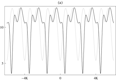
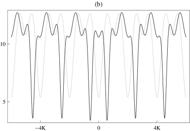
Figure 1: First-order SUSY partners (black curves) for the associated Lamé potential (gray curves) with $m=3,\ \ell=2$, $k^{2}=0.9$. (a) Periodic case generated through the Bloch solution $\psi^{+}(x)$ with $\epsilon=8$. (b) Asymptotically periodic case in which the linear combination $\psi^{+}(x)+\psi^{-}(x)$ for the same $\epsilon$ is used.

V Conclusions

We have shown that the associated Lamé potentials for integers values of the parameter pair $(m,\ell)$ are exactly solvable. When using as seeds Bloch-type solutions inside the gaps new exactly solvable periodic potentials are generated. On the other hand, for seeds chosen as general linear combinations of Bloch-type solutions, the SUSY partner potentials become asymptotically periodic, the corresponding spectra having bound states embedded into the gaps. These potentials are interesting since the new levels could work as intermediate transition energies for the electrons to jump between the energy bands.

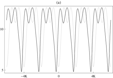
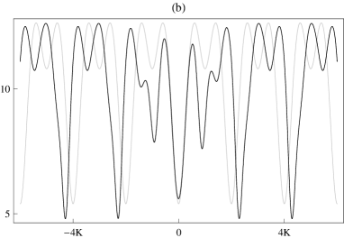
Figure 2: Second-order SUSY partners (black curves) for the associated Lamé potential (gray curves) with $m=3,\ \ell=2$, $k^{2}=0.9$. (a) Periodic case generated through two Bloch solutions $u_{1}(x)=\psi_{1}^{+}(x)$, $u_{2}(x)=\psi_{2}^{+}(x)$ for $\epsilon_{1}=10$, $\epsilon_{2}=10.1$. (b) Asymptotically periodic case in which the linear combinations $u_{1}(x)=\psi_{1}^{+}(x)+\psi_{1}^{-}(x)$, $u_{2}(x)=\psi_{2}^{+}(x)-1.5\ \psi_{2}^{-}(x)$ for the same $\epsilon_{1,2}$ are used.

We would like to end up this paper by making a historical precision concerning SUSY techniques applied to periodic potentials (see also the discussion in cjp08 ). It is a fact that the recent interest on the subject df98 ; ks99 ; fnn00 ; fmrs02a ; fmrs02b ; sgnn03 ; fg05 ; fg07 ; gin06 ; imv08 ; cjnp08 was catalyzed by Dunne and Feinberg discovery of the self-isospectrality for the Lamé potentials with $m=1$, induced by the first-order SUSY transformation which employs as seed the ground-state eigenfunction. Self-isospectrality means, in particular, that the SUSY partner potential becomes just a displaced version of the initial one, by half the period in df98 . Soon it was realized that the self-isospectrality in which the new potential becomes the initial one displaced by any real number arises as well for the Lamé potential with $m=1$, the seeds employed being Bloch-type solutions associated to factorization energies in the gaps fmrs02a ; fmrs02b . More general SUSY transformations, either of higher order or involving general solutions of the Schrödinger equation for a given factorization energy, have been also introduced fmrs02a ; fmrs02b ; sgnn03 . However, it is worth to note that there are several interesting works, previous to Dunne and Feinberg paper, in which the SUSY techniques were applied to periodic potentials (see e.g. tr89 ; bm85 ). In particular, it is remarkable the work of Braden and Macfarlane in which the self-isospectrality for the Lamé potential with $m=1$ was discovered for the first time bm85 . This is a typical story of a discovery followed by a later rediscovery, which often arises in science. Our opinion is that both works are valuable, complementary to each other, and hence they are worth to be studied in detail.

References

• (1) A.G. Ushveridze, Quasi-exactly solvable models in quantum mechanics, IOP Publishing Ltd, Bristol (1994)
• (2) S.S. Ranjani, A.K. Kapoor, P.K. Panigrahi, Int. J. Theor. Phys. 44 (2005) 1167
• (3) D.J. Fernández, A. Ganguly, Phys. Lett. A 338 (2005) 203
• (4) D.J. Fernández, A. Ganguly, Ann. Phys. 322 (2007) 1143
• (5) G. Dunne, J. Feinberg, Phys. Rev. D 57 (1998) 1271
• (6) A. Khare, U. Sukhatme, J. Math. Phys. 40 (1999) 5473
• (7) D.J. Fernández, J. Negro, L.M. Nieto, Phys. Lett. A 275 (2000) 338
• (8) D.J. Fernández, B. Mielnik, O. Rosas-Ortiz, B.F. Samsonov, Phys. Lett. A 294 (2002) 168
• (9) D.J. Fernández, B. Mielnik, O. Rosas-Ortiz, B.F. Samsonov, J. Phys. A 35 (2002) 4279
• (10) B.F. Samsonov, M.L. Glasser, J. Negro, L.M. Nieto, J. Phys. A 36 (2003) 10053
• (11) A.A. Andrianov, M.V. Ioffe, V.P. Spiridonov, Phys. Lett. A 174 (1993) 273
• (12) A.A. Andrianov, M.V. Ioffe, F. Cannata, J.P. Dedonder, Int. J. Mod. Phys. A 10 (1995) 2683
• (13) A. Ganguly, Mod. Phys. Lett. A 15 (2000) 1923
• (14) A. Ganguly, J. Math. Phys. 43 (2002) 1980
• (15) F. Correa, V. Jakubský, M. Plyushchay, J. Phys. A 41 (2008) 485303
• (16) A. Ganguly, M.V. Ioffe, L.M. Nieto, J. Phys. A 39 (2006) 14659
• (17) M.V. Ioffe, J. Mateos Guilarte, P.A. Valinevich, Nucl. Phys. B 790 (2008) 414
• (18) F. Correa, V. Jakubský, L.M. Nieto, M.S. Plyushchay, Phys. Rev. Lett. 101 (2008) 030403
• (19) H.W. Braden, A.J. Macfarlane, J. Phys. A 18 (1985) 3151
• (20) L. Trlifaj, Inv. Probl. 5 (1989) 1145