Regularization, Renormalization, and Dimensional Analysis:
Dimensional Regularization Meets Freshman E&M

Abstract

We illustrate the dimensional regularization (DR) technique using a simple problem from elementary electrostatics. This example illustrates the virtues of DR without the complications of a full quantum field theory calculation. We contrast the DR approach with the cutoff regularization approach, and demonstrate that DR preserves the translational symmetry. We then introduce a Minimal Subtraction ($MS$) and a Modified Minimal Subtraction ($\overline{MS}$) scheme to renormalize the result. Finally, we consider dimensional transmutation as encountered in the case of compact extra-dimensions.

I Dimensional Regularization

I.1 Introduction and Motivation

In 1999, Gerardus ’t Hooft and Martinus J.G. Veltman received the Nobel Prize in Physics(physicstoday1999Lubkin, ) “for elucidating the quantum structure of electroweak interactions in physics.” In particular, they demonstrated that the non-abelian electroweak theory could be consistently renormalized to yield unique and precise predictions.

A key ingredient for their demonstration was the development of the dimensional regularization technique.('tHooft:1972fi, ; 'tHooft:1973mm, ; Bollini:1972ui, ) That is, instead of working in precisely D=4 space-time dimensions, they generalized the dimension to be a continuous variable so they could compute the theory in D=4.01 or D=3.99 dimensions.

An important property of the dimensional regularization is that it respects gauge and Lorentz symmetries. This is in contrast to the other regularization schemes (e.g. cutoff schemes, etc.) which violate these symmetries. The symmetries of the electroweak theory play a critical role in determining the dynamics of the particles and their interactions. Because it respects these symmetries, dimensional regularization has become an essential tool for the calculation of field theories.

While dimensional regularization is a powerful and elegant technique, most examples and applications of dimensional regularization are in the context of complex higher-order Quantum Field Theory (QFT) calculations involving gauge and Lorentz symmetries. However, the virtues of dimensional regularization can be exhibited without the “distractions” of the associated QFT complexities.

In the present paper, we will apply the dimensional regularization method to a problem from an elementary undergraduate physics course, namely the electric potential of an infinite line of charge.(kaufman1969, ; Hans:1982vy, ) The example is simple enough for the undergraduate to understand, yet contains many of the concepts we encounter in a true QFT calculation. We will contrast the symmetry-preserving dimensional regularization approach with a symmetry-violating cutoff approach.

Imagining a variable number of dimensions can be a productive exercise. To explain the weak nature of the gravitational force physicists have recently posited the existence of “Extra Dimensions.” Having considered space-time dimensions in the neighborhood of $D=4$, we briefly contemplate wider excursions of $D=4,5,6,...$ dimensions.

II Dimension Analysis: The Pythagorean Theorem

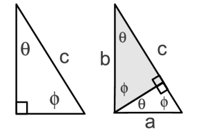
Figure 1: a) A right triangle specified by angles $\{\theta,\phi\}$ and hypotenuse $c$. b) The same triangular area can be described by two similar triangles of hypotenuse $a$ and $b$.

To illustrate utility of dimensional regularization and dimensional analysis, we warm-up with a pre-example. Our goal will be to demonstrate the Pythagorean Theorem, and our method will be dimensional analysis.

We consider the right triangle displayed in Fig. 1-a). From the Angle-Side-Angle (ASA) theorem, this can be uniquely specified using the two angles $\{\theta,\phi\}$ and the hypotenuse $c$. We now construct a formula for the area of the triangle, $A_{c}$, using only these variables: $\{c,\theta,\phi\}$. Note that $c$ has dimensions of length, and $\{\theta,\phi\}$ are dimensionless. From dimensional analysis, the area of the triangle must have dimensions of length squared. As $c$ is the only dimensional quantity, the formula for $A_{c}$ must be of the form:

$$A_{c}=c^{2}f(\theta,\phi)$$ (1)

where $f(\theta,\phi)$ is an unknown dimensionless function. Note that $f(\theta,\phi)$ cannot depend on the length $c$ as this would spoil the dimensionless nature of $f(\theta,\phi)$.

We now observe that we can divide the original triangle of Fig. 1-a) into two similar triangles of hypotenuse $a$ and $b$ as displayed in Fig. 1-b). Again, using the ASA theorem, we can represent the area of these triangles, $A_{a}$ and $A_{b}$, in terms of the variables $\{a,\theta,\phi\}$ and $\{b,\theta,\phi\}$, respectively. Again from dimensional considerations, these areas must be proportional to $a^{2}$ and $b^{2}$. Thus, we obtain:

$$A_{a}+A_{b}=a^{2}f(\theta,\phi)+b^{2}f(\theta,\phi)\quad.$$ (2)

Because all three triangles are similar, their areas are described by the same $f(\theta,\phi)$. It is important to note that the function $f(\theta,\phi)$ is universal, dimensionless, and scale-invariant.

Finally, we use “conservation of area” to obtain our result. Specifically, since the area of the original triangle $A_{c}$ is equal to the sum of the combined $A_{a}$ and $A_{b}$,

$$A_{a}+A_{b} = A_{c}\quad.$$ (3)

We can substitute Eqs. (1) and (2) to obtain our desired result:

$$a^{2}f(\theta,\phi)+b^{2}f(\theta,\phi) = c^{2}f(\theta,\phi)$$

$$a^{2}+b^{2} = c^{2}\quad.$$ (4)

The last equation is, of course, the Pythagorean Theorem. Clearly, there are much simpler methods to prove this theorem; however, this method does illustrate the power of the dimensional analysis approach. Additionally, we gain a new perspective on the Pythagorean Theorem in this proof as it is linked to conservation of area.

There are instances, such as renormalizable field theory, where dimensional analysis tools are essential to making certain calculations tractable. The following example will illustrate some of these features.

III An Infinite Line of Charge

III.1 Statement of the Problem

Figure 2: Coordinate system for an infinite line of charge running in the $y$-direction with linear charge density $\lambda=dQ/dy$. We compute the potential $V(x)$ at a fixed perpendicular distance $x$ from the line of charge. The distance to the element of charge $dQ$ is $r=\sqrt{x^{2}+y^{2}}$.

For our next example we consider the calculation of the electric potential $V$ for the case of an infinite line of charge with constant linear charge density $\lambda=dQ/dy$. The contribution to the electric potential from an infinitesimal charge $dQ$ is given by:

$$dV=\,\frac{1}{4\pi\epsilon_{0}}\,\frac{dQ}{r}\quad.$$ (5)

We choose our coordinate system (cf. Fig. 2) such that $x$ specifies the perpendicular distance from the wire, $y$ is the coordinate along the wire, and $r=\sqrt{x^{2}+y^{2}}$. Given $\lambda=dQ/dy$ we have $dQ=\lambda dy$ and can integrate along the length of the wire to obtain:

$$V(x) = \frac{\lambda}{4\pi\epsilon_{0}}\int_{-\infty}^{+\infty}\frac{dy}{\sqrt{x^{2}+y^{2}}}=\infty\quad.$$ (6)

Unfortunately, this integral is logarithmically divergent and we obtain an infinite result.

III.2 Scale invariance:

If we take a closer look at this integral, we will demonstrate that it is scale invariant. That is, if we rescale the argument $x$ by a constant factor $k\;(x\to k\,x)$, the result is invariant.

$$V(k\,x) = \frac{\lambda}{4\pi\epsilon_{0}}\int_{-\infty}^{+\infty}dy\ \,\frac{1}{\sqrt{(k\,x)^{2}+y^{2}}}$$ (7)

$$= \frac{\lambda}{4\pi\epsilon_{0}}\int_{-\infty}^{+\infty}d(y/k)\,\frac{1}{\sqrt{x^{2}+(y/k)^{2}}}$$ (8)

$$= \frac{\lambda}{4\pi\epsilon_{0}}\int_{-\infty}^{+\infty}dz\,\frac{1}{\sqrt{x^{2}+z^{2}}}$$ (9)

$$= V(x)\quad.$$ (10)

In the above we have implemented the rescaling $z=y/k$. Since both $y$ and $z$ are dummy variables and the integration limits are infinite, the integral is unchanged. A consequence of this scale invariance is:

$$V(x_{1}) = V(x_{2})\quad.$$ (11)

At first glance, this result appears to be a disaster since the usual purpose of the electric potential is to compute the work $W$ via the formula

$$W/Q=\Delta V=V(x_{2})-V(x_{1})$$ (12)

or to compute the electric field via

$$\vec{E}=-\vec{\nabla}V\quad.$$ (13)

As Eq. (11) suggests $V(x_{2})-V(x_{1})=0$, this implies that our attempts to compute the work $W$ or the electric field $\vec{E}$ will be meaningless.

We now understand why it is fortunate that $V(x)$ is infinite as infinite numbers have some unusual properties. For example, given a finite constant $c$ we can write (schematically) $\infty+c=\infty$ which implies $\infty-\infty=c$. We now understand that even though we have $V(x_{1})=V(x_{2})$, because these quantities are infinite we can still find that the difference is non-zero: $\delta V=V(x_{2})-V(x_{1})\not=0$. The challenge is that the difference of two infinite quantities is ambiguous. That is, how can we tell if $\infty-\infty=c_{1}$ or $\infty-\infty=c_{2}$ is the correct physical result?

The solution is that we must regularize the infinite quantities so that we can uniquely extract the difference.

IV Cutoff Regularization:

IV.1 Cutoff Regularization Computation

We will first regularize the integral using a simple cutoff method. That is, instead of considering an infinite wire, we will compute the potential for a finite wire of length $2L$. In this instance, the potential becomes:

$$V(x) = \frac{\lambda}{4\pi\epsilon_{0}}\int_{-L}^{+L}dy\frac{1}{\sqrt{x^{2}+y^{2}}}$$ (14)

$$= \frac{\lambda}{4\pi\epsilon_{0}}{\rm Log}\left[\frac{+L+\sqrt{L^{2}+x^{2}}}{-L+\sqrt{L^{2}+x^{2}}}\right]\quad.$$

We make the following observations.

• The result is finite.

• In addition to the physical length scale $x$, $V(x)$ depends on an artificial regulator $L$.

• We cannot remove the regulator $L$ without $V(x)$ becoming singular.

• The result for $V(x)$ violates a symmetry of the original problem—translation invariance.

IV.2 Computation of $E$ and $\delta V$

Even though $V(x)$ depends on the artificial regulator $L$, we observe that all physical quantities are independent of this regulator in the limit $L\to\infty$. Specifically, for the electric field we have:

$$E(x) = \frac{-\partial V(x)}{\partial x}=\frac{\lambda}{2\pi\epsilon_{0}x}\frac{L}{\sqrt{L^{2}+x^{2}}}$$ (15)

$$\ {\longrightarrow\atop{\scriptstyle{L\to\infty}}}\ \frac{\lambda}{2\pi\epsilon_{0}x}$$

and for the potential difference (proportional to the electric work $W$) we have:

$$\delta V = V(x_{1})-V(x_{2}){\longrightarrow\atop{\scriptstyle{L\to\infty}}}\ \frac{\lambda}{4\pi\epsilon_{0}}{\rm Log}\left[\frac{x_{2}^{2}}{x_{1}^{2}}\right]\quad.$$ (16)

As we observed in Sec. III.2, $\delta V$ is finite even though it is the difference of two infinite terms $V(x_{1})$ and $V(x_{2})$. The regulator $L$ allows us unambiguously to extract the finite difference $\delta V$, at which point the regulator can be discarded ($L\to\infty$). The fact that the physical quantities $E(x)$ and $\delta V$ are independent of the unphysical regulator is a essential property of any regularization method. We will discuss this further in Sec. VII.

IV.3 Broken Translational Symmetry:

Notice that the presence of the cutoff $L$ breaks the translation symmetry of the original problem. That is, for a truly infinite wire, our position in the $y$-direction is inconsequential; however, for a finite wire this is no longer the case. Specifically, if we shift our $y$-position by a constant $c$ to $y\to y^{\prime}=y+c$, our result becomes:

$$V(x) = \frac{\lambda}{4\pi\epsilon_{0}}\int_{-L+c}^{+L+c}dy\frac{1}{\sqrt{x^{2}+y^{2}}}$$

$$= \frac{\lambda}{4\pi\epsilon_{0}}{\rm Log}\left[\frac{+(L+c)+\sqrt{(L+c)^{2}+x^{2}}}{-(L-c)+\sqrt{(L-c)^{2}+x^{2}}}\right]\quad.$$

Clearly we have lost the translation invariance $y\to y^{\prime}=y+c$.

While preserving symmetries is not of paramount importance in this simple example, it is essential for certain field theory calculations. We now repeat this calculation, but instead using dimensional regularization which will preserve the translational symmetry.

IV.4 Recap

In summary, we find that our problem is solved at the expense of 1) an extra scale $L$ which serves both to regulate the infinities and provide an auxiliary length scale, and 2) a broken symmetry—translational invariance.

V Dimensional Regularization

$n$	$\Omega_{n}$	$\Gamma(n/2)$	Object	$V_{n}$	Surface	$S_{n-1}$
1	$2$	$\sqrt{\pi}$	Line	$2R$	Point	$2$
2	$2\pi$	1	Disk	$\pi R^{2}$	Line	$2\pi R$
3	$4\pi$	$\frac{1}{2}\,\sqrt{\pi}$	3-Ball	$\frac{4\pi}{3}R^{3}$	2-Sphere	$4\pi R^{2}$
4	$2\pi^{2}$	1	4-Ball	$\frac{\pi^{2}}{2}R^{4}$	3-Sphere	$2\pi^{2}R^{3}$
5	$\frac{8\pi^{2}}{3}$	$\frac{3}{4}\,\sqrt{\pi}$	5-Ball	$\frac{8\,\pi^{2}}{15}R^{5}$	4-Sphere	$\frac{8\pi^{2}}{3}R^{4}$

Table 1: Angular integration measure $\Omega_{n}$ as a function of dimension $n$. The surface of the $n$-dimensional volume $V_{n}$ is an $(n-1)$-dimensional manifold $S_{n-1}$. We recognize $\Omega_{2}$ as the circumference of the unit circle, $\Omega_{3}$ as the surface area of the unit sphere, and $\Omega_{4}$ as the 3-surface of the 4-dimensional unit hypersphere. See Appendix X for details.

V.1 Generalization to Arbitrary Dimension

The central idea of dimensional regularization is to compute $V(x)$ in $n$-dimensions where $n$ is not necessarily an integer.(Bollini:1972ui, ; 'tHooft:1973mm, ; 'tHooft:1972fi, ) We can generalize the integration of Eq. (6) by replacing the one-dimensional integration $\int dy$ by the general $n$-dimension result. Specifically, we make the replacement:

$$\int_{-\infty}^{+\infty}\,dy=\int dV_{1}\longrightarrow\int dV_{n}=\int d\Omega_{n}\,\int_{0}^{+\infty}y^{n-1}dy\,.$$ (18)

where the angular integration measure is given by

$$\Omega_{n}=\int d\Omega_{n} = \frac{2\pi^{n/2}}{\Gamma\left(\frac{n}{2}\right)}\equiv\frac{n\,\pi^{n/2}}{\Gamma\left(\frac{n}{2}+1\right)}\quad.$$ (19)

Here, $\Omega_{n}$ is the solid-angle in $n$-dimensions, and we have used $\Gamma(z+1)=z\,\Gamma(z)$ where $\Gamma$ is the Gamma function. In Appendix X we provide additional explanation, and verify that $\Omega_{n}$ yields the expected results for integer dimensions as tabulated in Table 1.

V.2 Computation of V in arbitrary dimensions

The generalized formula for $V(x)$ now reads:(Hans:1982vy, )

$$V(x) = \frac{\lambda}{4\pi\epsilon_{0}}\int\,d\Omega_{n}\int_{0}^{+\infty}\ \frac{y^{n-1}}{\mu^{n-1}}\ \frac{dy}{\sqrt{x^{2}+y^{2}}}\,.$$ (20)

Note that we are forced to introduce an auxiliary scale factor of $\mu^{n-1}$, where $\mu$ has units of length, to ensure $V(x)$ has the correct dimension. Replacing $n=1-2\epsilon$ to facilitate expanding about $n=1$ we obtain

$$V(x) = \frac{\lambda}{4\pi\epsilon_{0}}\frac{\Gamma\left[\frac{1-n}{2}\right]}{\left(\frac{x}{\mu}\sqrt{\pi}\right)^{1-n}}$$ (21)

$$= \frac{\lambda}{4\pi\epsilon_{0}}\left(\frac{\mu^{2\epsilon}}{x^{2\epsilon}}\,\frac{\Gamma[\epsilon]}{\pi^{\epsilon}}\right)\quad.$$

We make the following observations about the dimensionally regularized result.

• $V(x)$ depends on an artificial regulator $\epsilon$ which is dimensionless.

• $V(x)$ depends on an auxiliary scale $\mu$ which has dimensions of length.

• If we remove either the regulator $\epsilon$ or the auxiliary scale $\mu$ then $V(x)$ will become ill-defined.

• The dimensional regularization preserves the translation invariance of the original problem.

It is interesting to contrast this result with the cutoff regularization method where $L$ serves as both the regulator and the auxiliary scale.

V.3 Computation of $E$ and $\delta V$

For the potential difference we find

$$\delta V = V(x_{1})-V(x_{2}){\longrightarrow\atop\epsilon\to 0}\ \frac{\lambda}{4\pi\epsilon_{0}}{\rm Log}\left[\frac{x_{2}^{2}}{x_{1}^{2}}\right]$$ (22)

and for the electric field we obtain:

$$E = \frac{-\partial V(x)}{\partial x}=\frac{\lambda}{4\pi\epsilon_{0}}\left[\frac{2\epsilon\mu^{2\epsilon}\Gamma[\epsilon]}{\pi^{\epsilon}x^{1+2\epsilon}}\right]$$ (23)

$${\longrightarrow\atop\epsilon\to 0} \ \frac{\lambda}{2\pi\epsilon_{0}}\,\frac{1}{x}\quad.$$

As before, we observe that all physical quantities are independent of both the regulator $\epsilon$ and the auxiliary scale $\mu$.

V.4 Recap

In conclusion we find that the problem for $V(x)$ is solved at the expense of an artificial regulator $\epsilon$ and an auxiliary scale $\mu$. We also note the regulator $\epsilon$ and auxiliary scale $\mu$ are separate entities in contrast to the cutoff regularization method where the length $L$ plays both roles. Additionally, translational invariance symmetry is preserved. The fact that dimensional regularization respects symmetries makes this technique indispensable for field theory calculations involving gauge symmetries and Lorentz symmetries.

VI Renormalization

Having demonstrated two separate methods to regularize the infinities that enter the calculation of $V(x)$, we now turn to renormalization.

While physical quantities such as the work $W\sim\delta V$ and the electric field $\vec{E}\sim-\vec{\nabla}V$ are derived from $V(x)$, the potential itself is not a physical quantity. In particular, we can shift the potential by a constant $c$, $V\to V+c$, and the physical quantities will be unchanged.

To illustrate this point, let’s expand $V(x)$ of Eq. (21) in powers of $\epsilon$:

$$V(x) = \frac{\lambda}{4\pi\epsilon_{0}}\left[\frac{1}{\epsilon}+\ln\left[\frac{e^{-\gamma_{E}}}{\pi}\right]+\ln\left[\frac{\mu^{2}}{x^{2}}\right]+{\cal O}(\epsilon)\right]\,.$$

Here, $\gamma_{E}\simeq 0.577216$ is the Euler constant which arises from expanding the Gamma function $\Gamma[\epsilon]\sim\frac{1}{\epsilon}-\gamma_{E}$.

Let us now invent a Minimal Subtraction (MS) prescription. We have the freedom to shift $V(x)$ by a constant, and we choose this constant to eliminate the $1/\epsilon$ term:

$$V_{MS}(x) = \frac{\lambda}{4\pi\epsilon_{0}}\left[\phantom{\frac{1}{\epsilon}+}\ln\left[\frac{e^{-\gamma_{E}}}{\pi}\right]+\ln\left[\frac{\mu^{2}}{x^{2}}\right]+{\cal O}(\epsilon)\right]\,.$$

We can go even further and invent a Modified Minimal Subtraction ($\overline{MS}$) prescription to eliminate the $\ln[e^{-\gamma_{E}}/\pi]$ term as well:

$$V_{\overline{MS}}(x) = \frac{\lambda}{4\pi\epsilon_{0}}\left[\phantom{\frac{1}{\epsilon}+\ln\left[\frac{e^{-\gamma_{E}}}{\pi}\right]+}\ln\left[\frac{\mu^{2}}{x^{2}}\right]+{\cal O}(\epsilon)\right]\,.$$

After renormalization we can remove the regulator ($\epsilon\to 0$), but not the auxiliary scale $\mu$. Recall that without an auxiliary scale to generate a dimensionless ratio $\mu/x$ we could not have any substantive $x$-dependence.

In addition to the $\mu$-dependence we will also have renormalization scheme dependence in $V(x)$. However, physical observables must be independent of the auxiliary scale $\mu$ and the particular renormalization scheme. For example, the computed potential differences yield identical results when calculated consistently in a single renormalization scheme:

$$V_{MS}(x_{1})-V_{MS}(x_{2}) = \delta V=V_{\overline{MS}}(x_{1})-V_{\overline{MS}}(x_{2})\quad.$$

Here, the results of the Minimal Subtraction (MS) and the Modified Minimal Subtraction ($\overline{MS}$) are identical for physical quantities.

However, if you mix renormalization schemes inconsistently you will obtain non-sensible results that are dependent on the choice of scheme:

$$V_{\overline{MS}}(x_{1})-V_{MS}(x_{2}) \not= \delta V\not=V_{MS}(x_{1})-V_{\overline{MS}}(x_{2})\quad.$$

VI.1 Connection to QFT

This elementary problem of the infinite line charge contains all the key concepts of the dimensional regularization and renormalization that we encounter in the full QFT radiative calculations. For example, in the radiative Quantum Chromodynamics (QCD) calculation of the Drell-Yan process ($q\bar{q}\to\gamma^{*}\to\mu^{+}\mu^{-}$) we encounter the following infinite expression:

$$\frac{D(\epsilon)}{\epsilon} = \left(\frac{4\pi\mu^{2}}{Q^{2}}\right)^{\epsilon}\,\frac{\Gamma(1-\epsilon)}{\Gamma(1-2\epsilon)}$$ (29)

$$\sim \frac{1}{\epsilon}-\ln\left(\frac{e^{+\gamma_{E}}}{4\pi}\right)+\ln\left(\frac{\mu^{2}}{Q^{2}}\right)\quad.$$

In this equation, $Q$ represents the characteristic energy scale. This is the independent variable that is analogous to $x$ in our example. While this is for a 4-dimensional QCD calculation, the structure of the divergent term is remarkably similar to our simple one-dimensional example above. For the QCD calculation, the Minimal Subtraction ($MS$) prescription for this Drell-Yan calculation eliminates the $1/\epsilon$ term, and the Modified Minimal Subtraction ($\overline{MS}$) prescription eliminates the $1/\epsilon-\ln[e^{+\gamma_{e}}/(4\pi)]$ so that only the $\ln[\mu^{2}/Q^{2}]$ remains.

VII The Renormalization Group Equation

VII.1 Physical Observables:

The fact that the physical observables are independent of the unphysical auxiliary scale $\mu$ is simply a consequence of the renormalization group equation (RGE):

$$\mu\,\frac{d\sigma}{d\mu} = 0$$ (30)

where $\sigma$ represents any physical observable. Thus, the renormalization group equation implies that the electric field $\vec{E}=\vec{\nabla}V$ and the work $W=\delta V$ are also independent of the $\mu$ scale:

$$\mu\,\frac{dE}{d\mu}=0\qquad\qquad\mu\,\frac{dW}{d\mu}=0\quad.$$ (31)

These results are implicit in the final expression for the physical quantities $E$ and $V$.

VII.2 Relating Perturbative & Non-Perturbative Functions

While the result of Eq. (30) appears to be almost trivial in the above example, this yields a very important result when applied to scattering processes involving non-perturbative hadronic particles (proton, nucleons, etc.). We can write the physical cross section $\sigma$ as a product of a non-perturbative distribution $f$ which describes the soft (low energy) physics, and a perturbative term $\omega$ which describes the hard (high energy) physics:

$$\sigma=f\,\omega\quad.$$ (32)

Differentiating with respect to $\ln\mu$ and applying the chain rule we find

$$\frac{d\sigma}{d\ln\mu}=0=\frac{df}{d\ln\mu}\,\omega+f\,\frac{d\omega}{d\ln\mu}$$ (33)

where we have used Eq. (30). Rearranging terms, we place all the $f$ dependence on the left-hand-side (LHS) and the $\omega$ dependence on the right-hand-side (RHS),

$$\frac{1}{f}\,\frac{df}{d\ln\mu}=-\gamma=\frac{1}{\omega}\,\frac{d\omega}{d\ln\mu}\quad.$$ (34)

We introduce a separation constant $-\gamma$. We note the LHS of Eq. (34) depends only on the non-perturbative quantity $f$; therefore, the LHS is (in principle) incalculable. Conversely, the RHS of Eq. (34) depends only on the perturbative quantity $\omega$. Therefore, the RHS is calculable in perturbation theory, and we can use this to compute $-\gamma$.

Having computed $-\gamma$, we can solve Eq. (34) for $f$ to obtain

$$f\sim\mu^{-\gamma}\quad.$$ (35)

Equation (35) is a remarkable result! Even though $f$ was an incalculable non-perturbative quantity, we are able to find the $\mu$-dependence for this function. Thus, the renormalization group equation has allowed us to compute the $\mu$-dependence of an incalculable quantity by relating the (incalculable) non-perturbative $df/f$ to the (calculable) perturbative $d\omega/\omega=-\gamma$.

VIII Extra Dimensions

$D_{{\rm eff}}$	$E(r)$	$V(r)$	Example
3	$\frac{1}{r^{2}}$	$\frac{1}{r}$	Point charge
2	$\frac{1}{r^{1}}$	$\ln\,r$	Line charge
1	$\frac{1}{r^{0}}$	$r$	Sheet charge

Table 2: Example charge configurations that illustrate $D_{{\rm eff}}=\{3,2,1\}$ effective dimensions.

VIII.1 E and V in arbitrary dimensions

In the above example, we used the mathematical trick of generalizing the number of integration dimensions from an integer to a continuous parameter. While we only let the dimension stray by $2\epsilon$, it is useful to consider more drastic shifts as in the case of “Extra-Dimensions” which have recently been hypothesized.(ArkaniHamed:1998rs, ; Randall:1999ee, ) In this section, we provide an example of a dimensional transmutation where the effective dimension $D_{{\rm eff}}$ changes from one integer to another as we probe the system at different scales.

For example, we can generalize the $r$-dependence of the potential and electric field in for the case of $D$-dimensions as:

$$V(r)\sim\frac{1}{r^{D-2}}\qquad\qquad E(r)\sim\frac{1}{r^{D-1}}\quad.$$ (36)

A quick check will verify that this reproduces the usual expressions in ordinary $D=3$ spacial dimensions. Additionally, in 3-dimensions we can create charge distributions that mimic lower order spatial dimensions. This is illustrated in Table 2. For a (zero-dimensional) point-charge in 3-dimensions, according to Gauss’s law the electric field lines spread out on a surface of $D-1=2$ dimensions, and we observe $E(r)\sim 1/r^{2}$. Similarly, for a (one-dimensional) line-charge, our space is now effectively $D=2$ dimensional; hence the electric field lines spread out on a surface of $D-1=1$ dimension, and we observe $E(r)\sim 1/r$. Finally, for a (two-dimensional) sheet-charge, our space is now effectively $D=1$ dimensional; hence the electric field lines spread out on in $D-1=0$ dimensions, and we observe $E(r)\sim 1/r^{0}=constant$.

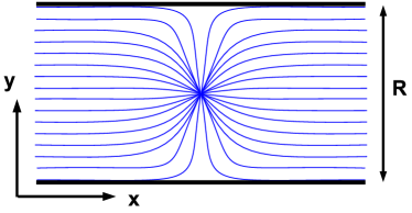
Figure 3: Electric field for a point charge confined in one infinite dimension $(x)$ and one finite dimension $(y)$ of scale $R$.

Figure 3 displays the electric field lines for a point charge confined to one infinite dimension $(x)$ and one finite (or compact) dimension $(y)$ of scale $R$. We observe that if we examine the electric field at scales small compared to the compact dimension $R$ $(r\ll R)$, we find the the electric field lines spread out in 2 dimensions and we obtain the usual 2-dimensional result $\vec{E}(r)\sim 1/r$. Conversely, if we examine the electric field at distance scales large compared to the compact dimension $R$ $(r\gg R)$, we find the 1-dimensional result $\vec{E}(r)\sim constant$. In this example, the effective dimension of our space changes as we move from small ($D=2$) to large length scales ($D=1$).

IX Conclusions

In this paper we have computed the potential of an infinite line of charge using dimensional regularization. By contrasting this calculation with the conventional cutoff approach, we demonstrated that dimensional regularization respects the symmetries of the problem—namely, translational invariance. The dimensional regularization requires that we introduce a regulator $\epsilon$ and an auxiliary length scale $\mu$. We then renormalized the potential to eliminate the $1/\epsilon$ singularities. This potential was finite and independent of the regulator $\epsilon$, but it depended on the particular renormalization scheme and renormalization scale $\mu$. However, we demonstrated that all physical observables $(E,\delta V)$ were scheme and scale invariant.

As this example exhibits many of the key features of dimensional regularization as applied to QFT, it provides an excellent opportunity to understand the virtues of this regularization method without the complications of gauge symmetries. As such, this example serves as an ideal pedagogical study.

X Appendix

X.1 3-Dimensions

The volume of a 3-sphere ($V_{3}$) in spherical coordinates is a product of the angular and radial integrals:

$$V_{3} = \int d\Omega_{3}\int_{0}^{R}r^{2}dr=\int_{0}^{2\pi}d\phi\int_{0}^{\pi}\sin\theta\,d\theta\int_{0}^{R}r^{2}dr$$ (37)

$$= \frac{4\pi}{3}R^{3}\quad.$$

Note that the angular integral $\int\Omega_{3}$ is dimensionless while the radial integral $\int r^{2}dr$ carries the dimensions.

For the 2-dimensional surface area ($S_{2}$), we can use the above $V_{3}$ integral with a $\delta$-function $\delta(r-R)$ to constrain us to the surface:

$$S_{2}=\int d\Omega_{3}\int_{0}^{R}dr\,r^{2}\delta(r-R)=4\pi R^{2}\quad.$$ (38)

X.2 $n$-Dimensions

Having established the familiar 3-dimensional case, we can generalize to $n$-dimensions:

$$V_{n}=\int d\Omega_{n}\,\int_{0}^{R}r^{n-1}dr=\Omega_{n}\frac{R^{n}}{n}$$ (39)

and the $(n-1)$-dimensional surface area ($S_{n-1}$) of the $n$-dimensional volume $V_{n}$ is:

$$S_{n-1}=\int d\Omega_{n}\,\int_{0}^{R}dr\,r^{n-1}\,\delta(r-R)=\Omega_{n}\,R^{n-1}\quad.$$ (40)

With the above we have the general relation:

$$\frac{V_{n}}{S_{n-1}}=\frac{R}{n}\quad.$$ (41)

Additionally, we find the following relation:

$$\frac{dV_{n}}{dR}=S_{n-1}\quad.$$ (42)

This demonstrates that the derivative (or boundary) of the volume is the surface area, $\partial V=S$.

X.3 1-Dimension

As the 1-dimensional case has a subtle factor of 2, we compute this explicitly. Using Eq. (39) we find the volume of a 1-dimensional line to be:

$$V_{1}=\int dV_{1}=\int d\Omega_{1}\,\int_{0}^{R}r^{0}\,dr=2R\quad.$$ (43)

Note, this result is not $R$ but $2R$ as the 1-dimensional line extends from $-R$ to $+R$.

In the notation of Eq. (6) we have (with $R\to\infty$)

$$\int dV_{1}=\int d\Omega_{1}\,\int_{0}^{+\infty}\,dy=2\int_{0}^{+\infty}\,dy=\int_{-\infty}^{+\infty}\,dy\quad.$$ (44)

Thus, we can make the replacement $\int_{-\infty}^{+\infty}\,dy\to\int dV_{1}$, and the $n$-dimensional generalization is then:

$$\int_{-\infty}^{+\infty}\,dy=\int dV_{1}\longrightarrow\int dV_{n}=\int d\Omega_{n}\,\int_{0}^{+\infty}y^{n-1}dy\,.$$ (45)

Eq. (6) for the potential $V(x)$ then becomes:

$$V(x) = \frac{\lambda}{4\pi\epsilon_{0}}\int d\Omega_{n}\,\int_{0}^{+\infty}y^{n-1}\frac{dy}{\sqrt{x^{2}+y^{2}}}\quad.$$ (46)

Note that Eq. (46) is not dimensionally correct as the factor $y^{n-1}$ will need to be compensated by introducing an auxiliary scale factor as we do in Eq. (20).

References

- (1) Gloria B. Lubkin. Nobel Prize to ’t Hooft and Veltman for Putting Electroweak Theory on Firmer Foundation. Physics Today, 52:17, 1999.
- (2) Gerard ’t Hooft, M. J. G. Veltman. Regularization and Renormalization of Gauge Fields. Nucl. Phys., B44:189–213, 1972.
- (3) Gerard ’t Hooft. Dimensional regularization and the renormalization group. Nucl. Phys., B61:455–468, 1973.
- (4) C. G. Bollini, J. J. Giambiagi. Dimensional Renormalization: The Number of Dimensions as a Regularizing Parameter. Nuovo Cim., B12:20–25, 1972.
- (5) C. Kaufman. An Illustration from Classical Physics of Renormalization Mathematics. Am. J. Phys., 37:560–561, 1969.
- (6) M. Hans. An electrostatic example to illustrate dimensional regularization and renormalization group technique. Am. J. Phys., 51:694–698, 1983.
- (7) Arkady B. Migdal. Qualitative Methods in Quantum Theory. Front. Phys., 48:1–437, 1977.
- (8) Steven Vogel. Exposing Life’s Limits with Dimensionless Numbers. Physics Today, 51:22–27, 1998.
- (9) Steven Vogel. Cats’ Paws and Catapults: Mechanical Worlds of Nature and People. Norton & Co., 2000.
- (10) Matt A. Bernstein, William A. Friedman. Thinking About Equations: A Practical Guide for Developing Mathematical Intuition in the Physical Sciences and Engineering, 2009. ISBN-13: 978-0470186206.
- (11) B. Potter. Calculational techniques in perturbative QCD: The Drell-Yan process. unknown, 1998. http://citeseer.ist.psu.edu/209991.html.
- (12) Bertrand Delamotte. A hint of renormalization. Am. J. Phys., 72:170–184, 2004.
- (13) Nima Arkani-Hamed, Savas Dimopoulos, G. R. Dvali. The hierarchy problem and new dimensions at a millimeter. Phys. Lett., B429:263–272, 1998.
- (14) Lisa Randall, Raman Sundrum. A large mass hierarchy from a small extra dimension. Phys. Rev. Lett., 83:3370–3373, 1999.