Investigating the potential of the Pan-Planets project using Monte Carlo simulations

Abstract

Using Monte Carlo simulations we analyze the potential of the upcoming transit survey Pan-Planets. The analysis covers the simulation of realistic light curves (including the effects of ingress/egress and limb-darkening) with both correlated and uncorrelated noise as well as the application of a box-fitting-least-squares detection algorithm. In this work we show how simulations can be a powerful tool in defining and optimizing the survey strategy of a transiting planet survey. We find the Pan-Planets project to be competitive with all other existing and planned transit surveys with the main power being the large 7 square degree field of view. In the first year we expect to find up to 25 Jupiter-sized planets with periods below 5 days around stars brighter than V = 16.5 mag. The survey will also be sensitive to planets with longer periods and planets with smaller radii. After the second year of the survey, we expect to find up to 9 Warm Jupiters with periods between 5 and 9 days and 7 Very Hot Saturns around stars brighter than V = 16.5 mag as well as 9 Very Hot Neptunes with periods from 1 to 3 days around stars brighter than i’ = 18.0 mag.

1 Introduction

Thirteen years after the first discovery of a planet revolving around a main-sequence star (Mayor & Queloz, 1995) more than 300 extra solar planets are known. The majority of these have been detected by looking for periodic small amplitude variations in the radial velocity of the planet’s host star. This method reveals the period, semi-major axis and eccentricity of the planetary orbit, but due to a generally unknown inclination only the minimum mass of the planet can be derived. The situation is different in the case of a planet that transits its host star. The planet blocks a small fraction of the stellar surface resulting in a periodic drop in brightness. In combination with radial velocity measurements the light curve provides many additional parameters like inclination, true mass and radius of the planet.
Transiting planets are subject of many detailed follow-up studies such as measurement of thermal emission using the secondary transit (Charbonneau et al., 2008; Knutson et al., 2008) or measurement of the spin-orbit alignment using the Rossiter-McLaughlin effect (e.g. Winn et al., 2007).
In the past years many transit projects have monitored hundreds of thousands of stars looking for periodic drops in the light curves. A total of about 50 transiting planets are known to date. Remarkably, more than half of the transiting planets have been found in the past year making the transit method equally successful in that period compared to the radial velocity method.
The majority of the recently detected transiting planets have been found by wide-angle surveys targeting bright stars such as WASP, HAT, TrES or XO (Pollacco et al., 2006; Noyes et al., 2008; O’Donovan et al., 2007; McCullough et al., 2005). Also the space mission Corot has contributed by adding four new discoveries (Aigrain et al., 2008). Deep surveys like OGLE targeting highly crowded regions of the Milky Way disk have not been able to keep up with the increased detection rate of all-sky monitoring programs mainly due to limited amount of observation time and a lower number of target stars.
In 2009 Pan-Planets - a new deep transit survey - will start taking first observations. This project will be more powerful than all existing deep surveys because of its by far larger field of view, bigger telescope and faster readout.

With the first detections of transiting extra-solar planets, several groups have started to predict the number of planets that could be found by existing and planned surveys. First estimates were based on optimistic assumptions and have been mostly over-predictions (e.g. Horne, 2003). For example the frequency of very close-in planets had been extrapolated from the metallicity biased results of the radial velocity surveys. Late type dwarfs with higher metallicity turned out to have a higher frequencies of close-in planets (Fischer & Valenti, 2005) and therefore transit surveys find less planets compared to radial velocity surveys due to a lower average metallicity (Gould et al., 2006). It was further assumed that planets could be found around all stars in the target fields whereas planets transiting giants show a much too faint photometric signal due to the larger radius of the star. In addition, the efficiency of the detection algorithm was not taken into account and all light curves with 2 visible transits were assumed to lead to a detection which is not the case.
More realistic methods have been introduced by Pepper et al. (2003) and Gould et al. (2006). Both groups use an analytical approach assuming a stellar and a planetary distribution and integrating over period, stellar mass, planetary radius and volume probed taking into account the detection probability. Similarly, Fressin et al. (2007) modeled the OGLE survey and compared the predicted distributions to the parameters actually found by OGLE. In a recent study, Beatty & Gaudi (2008) generalized the formalism of Gould et al. (2006) in order to provide a method that can be used to calculate planet yields for any photometric survey given the survey parameters like number of nights observed, bandpass, exposure time, telescope aperture, etc. They applied their method to a number of different planned surveys like SDSS-II and the Pan-STARSS 3$\pi$ survey.
In this work we use Monte Carlo simulations to predict the number of planets of the Pan-Planets survey. Our approach is quite general and applicable to any transit survey. Based on stellar and planetary populations we model the survey by constructing realistic light curves and running a detection algorithm on them. In this way we are able to directly include the effects of limb darkening, ingress/egress and observational window functions which have not been included in most previous studies. In addition we introduce a model for correlated noise and study its impact on the efficiency of the detection algorithm.
To optimize the survey strategy of Pan-Planets we want to address the following questions: What is the best observing block size (1h or 3h) and how many fields (3 to 7) should we observe? Given the optimized survey strategy, we study how many Very Hot Juptiters (VHJ) and Hot Jupiters (HJ) are expected in the first year and what is the potential of Pan-Planets to find planets with longer periods, such as Warm Jupiters (WJ) or planets with smaller radii, such as Very Hot Saturns (VHS) and Very Hot Neptunes (VHN). We further study whether it will be more efficient to observe the same target fields in the second year of the Pan-Planets survey or to choose new ones.

In §2 we give a brief overview of the Pan-Planets survey. §3 describes in detail the simulations we performed. We present our results in §4. In order to verify our results we perform a consistency check with the OGLE-III survey by comparing our predicted yield with the actual number of planets found (§5). Finally we draw our conclusions in §6.

2 Pan-Planets overview

The Panoramic Survey Telescope and Rapid Response System (PanSTARRS) is an Air Force funded project aiming at the detection of killer asteroids that have the potential of hitting the Earth in the near future. The prototype mission PanSTARRS1 is using a 1.8m telescope at the Haleakala Observatories (Maui, Hawaii) to monitor 3$\pi$ of the sky over a 3.5 yr period starting in early 2009. The telescope is equipped with the largest CCD camera in the world to date that samples a field of 7 sq.deg. on a 1.4 Gigapixel array (Kaiser, 2004) with a pixel-size of 0.258 arcsec.
To make use of the large amount of data that will be collected, a science consortium of institutes from USA, Germany, UK and Taiwan has defined 12 Key Science Projects, out of which one is the Pan-Planets transit survey. A total of 120h per year have been dedicated to this project during the 3.5 yr lifetime of the survey. The actual observing time will be less due to bad weather and technical downtime. We account for a 33% loss in our simulations.
In the first 2 years, Pan-Planets will observe 3 to 7 fields in the direction of the Galactic plane. Exposure and read-out time will be 30s and 10s respectively. The observations will be scheduled in 1h or 3h blocks. The target magnitude range will be 13.5 to 16.5 mag in the Johnson V-band. The magnitude range is extended to i’ = 18 when searching for Very Hot Neptunes (see §4.6). More detailed informations about Pan-Planets are presented in Afonso et al. (in prep.).

3 Description of the simulations

The goal of this work is to study the expected number of planets that will be detected by the Pan-Planets project as a function of different survey strategies, with a variety of different parameters like number of fields (3 to 7), length of a single observing block (1h and 3h) and level of residual red noise (0 mmag, 1 mmag, 2 mmag, 3 mmag and 4 mmag). In total we simulate about 100 different combinations of these parameters for each of 5 different planet populations (see §3.2).
In our simulations we follow a full Monte-Carlo approach, starting with the simulation of light curves with realistic transit signals. Systematic effects coming from data reduction steps on image basis, such as differential imaging or PSF-photometry are taken into account by adding non-Gaussian correlated noise, the so called red noise (Pont et al., 2006), to our light curves (see §3.4). We apply a box-fitting-least-squares algorithm to all simulated light curves in order to test whether a transiting planet is detected or not.
For each star in the input stellar distribution (§3.1) we decide randomly whether it has a planet or not, depending on the fraction of stars having a planet of this type. In the case it has a planet, we randomly pick a planet from the input planet distribution (§3.2) and create a star-planet pair which is attributed a randomly oriented inclination vector resulting in a transiting or non-transiting orbit (the geometric probability for a transiting orbit depends on stellar radius and semi-major axis of the orbit).
In the case of a transiting orbit, the light curve is simulated based on stellar and planetary parameters and the observational dates we specified (see §3.5). The shape of the transit is calculated according to the formulae of Mandel & Agol (2002) and includes the effects of ingress/egress and limb-darkening. We add uncorrelated Gaussian (white) and correlated non-Gaussian (red) noise to our light curves. Details about our noise model are given in §3.3 and §3.4. After the simulation of the light curves, we apply our detection algorithm and our detection cuts as described in §3.6, and count how many planets we detect.
One simulation run is finished after each star has been picked once. In this way one run represents one possible outcome of the Pan-Planets survey. Since in the majority of cases the star has no planet or the inclination is such that no transits are visible, there are in general only a few transiting light curves per run. For each planet population and each set of survey parameters we simulate 25 000 runs. For the selected survey strategy we increase the precision to 100 000 runs. The numbers we list in our results are averages over these runs. The scatter of the individual outcomes allows us to derive errors for our estimates.

3.1 Input stellar distribution

We make use of a Besançon model (Robin et al., 2003) for the spectral type and brightness distributions of stars in our target fields. A model of 1 sq.deg centered around RA = $19^{h}47^{m}41^{s}_{\cdot}7$, DEC = $+17^{d}01^{m}52^{s}$ (l = 54.5, b = -4.2) is scaled to the actual survey area assuming a constant density. The parameters taken from the model are stellar mass $M_{star}$, effective temperature $T_{eff}$, surface gravity log $g$, metallicity $[Fe/H]$ and apparent MegaCam i’-band AB-magnitude $m_{i^{\prime}}$. The model also provides colors which we use to determine the apparent Johnson V-band magnitude $m_{V}$, according to the following formula derived by Smith et al. (2002) :

$$V=g^{\prime}-0.55\cdot(g^{\prime}-r^{\prime})-0.03$$ (1)

The stellar radii $R_{star}$ are calculated using log $g$ and $M_{star}$ according to $R_{star}$ = sqrt($G\times M_{star}$ / $g$). Furthermore, $T_{eff}$, log $g$, and $[Fe/H]$ are used to determine quadratic limb-darkening coefficients according to Claret (2004) which are based on synthetic ATLAS spectra (Claret, 2000).
In total we find 3 440 F, G, K and M dwarfs per sq.deg. that are not saturated (i.e. $m_{i^{\prime}}\geq$ 13 mag) and are brighter than our radial velocity follow-up limit (i.e. $m_{V}\leq$ 16.5 mag). Fig. 1 shows the input stellar distribution.
For VHN we extend the target magnitude range to $m_{i^{\prime}}\leq$ 18 mag. We find 34 000 M dwarfs in this range.

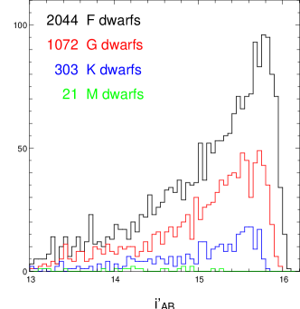
Figure 1: Total number and magnitude histogram for F, G, K and M dwarfs (top to bottom) with $m_{i^{\prime}}\geq$ 13 mag and $m_{V}\leq$ 16.5 mag in our target population. Note that the cut on the visual magnitude results in an brighter cut in i’ for the later type stars due to their redder color.

3.2 Input planet distributions

We test five different planetary populations :

1. Very Hot Jupiters (VHJ), with radii of 1.0-1.25 $R_{J}$ and periods between 1 and 3 days

2. Hot Jupiters (HJ), with radii of 1.0-1.25 $R_{J}$ and periods between 3 and 5 days

3. Warm Jupiters (WJ), with radii of 1.0-1.25 $R_{J}$ and periods between 5 and 10 days

4. Very Hot Saturns (VHS), with radii of 0.6-0.8 $R_{J}$ and periods between 1 and 3 days

5. Very Hot Neptunes (VHN), with radii of 0.3 $R_{J}$ and periods between 1 and 3 days

Within the given ranges the radii and periods are homogeneously distributed.
Our predicted yields depend on the frequency of stars that have a planet for each of the five population. These frequencies are not known to a very good precision and not many estimates have been published so far. Gould et al. (2006) performed a detailed study of the OGLE-III survey and derived frequencies of Very Hot Jupiters and Hot Jupiters by comparing the number of detected planets in the OGLE-III survey to the number of stars the survey was sensitive to. They found at 90% confidence level 0.1408 $\cdot$ ($1^{+1.10}_{-0.54}$)% of all late type dwarfs to have a VHJ and 0.3125 $\cdot$ ($1^{+1.37}_{-0.59}$)% to have an HJ. Fressin et al. (2007) published comparable results analyzing the same survey.
For VHJ and HJ we use the frequencies published by Gould et al. (2006). The frequency of WJ we speculate to be the same as for HJ which is consistent with the OGLE-III results (see §5). Further we assume the frequencies for VHS and VHN to be 0.714% (same as for VHJ) and 5% respectively.

3.3 White noise model

For the white noise in our light curves we add four different Gaussian components: stellar photon noise, sky background, readout and scintillation noise. The photon noise of each star is estimated using a preliminary exposure time calculator which has been calibrated by observations taken during a pre-commissioning phase of the PanSTARRS1 telescope. We assume the sky background to be 20.15 mag per square arcsecond which corresponds to a seven day distance to full moon. The readout noise is assumed to be 8 $e^{-}$ per pixel. The scintillation noise is estimated to be 0.5 mmag according to the formula of Young (1967, 1993) and is only of importance at the very bright end of our target distribution. Fig. 2 shows the white noise as function of magnitude as well as the individual contributions.
For our calculations we assume a seeing of 1.2 arcsec, airmass of 1.4, extinction coefficient of 0.08 and PSF fitting radius of 1.0 arcsec. At the faint end (i’ = 18 mag) the number of photons is on the order of 15,500 for the object and 7,800 for the sky and therefore well outside the Poisson statistics regime.

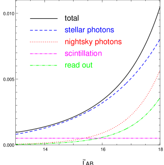
Figure 2: Total white noise and contributions of the four components.

3.4 Residual red noise model

As detailed analyses of light curve datasets have shown, all transit surveys suffer from non-Gaussian correlated noise sources, also known as red noise. E.g. Pont et al. (2006) analyzed the OGLE-III light curves and calculated binned averages of subsets containing n data points. They found the standard deviation $\sigma$ of these averages can be parameterized to a good approximation by the following formula :

$$\sigma=\sqrt{\frac{\sigma_{white}^{2}}{n}+\sigma_{red}^{2}}$$ (2)

with $\sigma_{white}$ being the single point rms of the white noise component and $\sigma_{red}^{2}$ being a constant red noise contribution. With this equation one can model how the red noise decreases the signal-to-noise ratio (S/N) of a transit light curve.
Application of algorithms to remove systematic effects, such as Sysrem (Tamuz et al., 2005) or TFA (Kovács et al., 2005) have been successfully applied by several groups resulting in a significant reduction of the level of red noise (e.g. Snellen et al., 2007). However, a small fraction of the correlated noise always remained.
In our simulations we want to account for this residual red noise (RRN). A simple model would be to increase the level of Gaussian noise by a certain amount and therefore assume that the correlated nature is of minor importance. For studies based only on S/N calculations one could also use a parameterization like equation 2. Since we are simulating light curves, we want to introduce a different approach. We model the RRN by adding superimposed sine waves of different wavelengths and amplitudes. This allows us to include the effects the correlated noise has on the efficiency of the detection algorithm, which could get confused by noise that is correlated on timescales of a typical transit duration.

We add RRN according to the following model :

$$\Delta_{flux}(t)=\sum\limits_{i}A_{i}\cdot sin(\frac{\pi}{\tau_{i}}t+p_{0,i})$$ (3)

with normalized amplitude $A_{i}$, timescale $\tau_{i}$ and random phase shift $p_{0,i}$ of each component i. The phase shift is calculated for each observing block independently and therefore changing with time for a single light curve. This is done in order to avoid introducing strong periodic signals that are coherent over a timescale longer than a day.
For each model we start with relative amplitudes $A_{i}^{\prime}$ which are normalized in such a way that the rms of the added RRN ($rms_{red}$) is of value 1 mmag, 2 mmag, 3 mmag or 4 mmag :

$$rms_{red}=\sqrt{\frac{\sum_{i}{A}_{i}^{2}}{2}}\quad.$$ (4)

In order to analyze the influence of the timescales and amplitudes on our results we construct a total of 9 different red noise models with each of them having 3 or 4 components. Table 1 gives an overview of the parameters of our red noise models. We refer to models 1 to 3 as ’fixed parameter’ models because for these we select arbitrary fixed values for $A_{i}^{\prime}$ and $\tau_{i}$ which we use for all light curve. For models 4 to 9 we draw the relative amplitudes and timescales randomly in a given range and for each light curve individually. Fig. 3 shows $\Delta_{flux}(t)$ for the fixed parameter models.

model number	$A_{1}^{\prime}$	$A_{2}^{\prime}$	$A_{3}^{\prime}$	$A_{4}^{\prime}$	$\tau_{1}$[min]	$\tau_{2}$[min]	$\tau_{3}$[min]	$\tau_{4}$[min]
1	1	2	3	4	355	169	111	48
2	2	3	4	1	169	131	111	88
3	3	4	1	2	131	99	61	27
4	random [1-4]	random [1-4]	random [1-4]	random [1-4]	random [300-400]	random [200-300]	random [100-200]	random [ 0-100]
5	random [1-4]	random [1-4]	random [1-4]	random [1-4]	random [250-300]	random [200-250]	random [150-200]	random [100-150]
6	random [1-4]	random [1-4]	random [1-4]	random [1-4]	random [250-300]	random [200-250]	random [150-200]	—
7	random [1-4]	random [1-4]	random [1-4]	random [1-4]	random [250-300]	random [200-250]	—	random [100-150]
8	random [1-4]	random [1-4]	random [1-4]	random [1-4]	random [250-300]	—	random [150-200]	random [100-150]
9	random [1-4]	random [1-4]	random [1-4]	random [1-4]	—	random [200-250]	random [150-200]	random [100-150]

Table 1: Dimensionless relative amplitudes $A_{i}^{\prime}$ and timescales $\tau_{i}$ of our different red noise models. Models 1 to 3 are fixed parameter models whereas for the others we draw random values within a given range for each single light curve individually. The timescales are chosen to cover the range of expected transit durations.

Figure 3: $\Delta_{flux}(t)$ for the fixed parameter models 1 to 3. Because the random phase shift is calculated for each day individually there are discontinuities visible at integer day positions (local noon). In our simulation we calculate the phase shift for each observing block in order to ensure continuity within an observing block.

3.5 Epochs of the observations

For each year the Pan-Planets survey has been granted a total of 120h hours which will be executed in 1h or 3h blocks. Assuming a 33% loss due to bad weather we expect the data to be taken in 81 or 27 nights per year depending on our survey strategy. The actual epochs of the observations we use to construct our light curves are computed in the following way. For each night in which our target field is visible for at least 3h we calculate the range of visibility, namely the time the field is higher than airmass 2 on the sky. This results in a 183 day period starting on April 26th and ending on October 24th. We randomly pick nights during the period of visibility and place the observing block arbitrarily within the time span our target is higher than airmass 2, as calculated earlier.
In our simulations we test 5 different scenarios with alternate observations of 3 to 7 fields during the observing block. The time for one exposure and readout is assumed to be 40s. Therefore the different number of fields transform into cycle rates between 120s and 280s. Using the selected nights, the random position of a block within a night and the cycle rate we construct a table of observational dates which we use as input to the light curve simulations. For each simulation run (which represents one possible outcome of the survey) we draw new observational dates. Table 2 summarizes the observational parameter depending on the survey strategy.

# of fields	block size	cycle rate	# of data points	# of data points
			per night	per year
3	1h	120s	30	2430
4	1h	160s	23	1863
5	1h	200s	18	1458
6	1h	240s	15	1215
7	1h	280s	13	1053
3	3h	120s	90	2430
4	3h	160s	68	1863
5	3h	200s	54	1458
6	3h	240s	45	1215
7	3h	280s	39	1053

Table 2: Cycle rate and number of data points per night and year depending on observational strategy.

3.6 Light curve analysis

Each simulated light curve is analyzed by our detection algorithm which is a box-fitting-least-squares (BLS) algorithm proposed by Kovács et al. (2002). The program folds the light curves with trial periods in the range from 0.9 to 9.1 days and finds the best $\chi^{2}$ fitting box corresponding to a fractional transit length $\tau$ between 0.01 and 0.1. For each detection the BLS algorithm provides period, S/N and the number of individual transits. For a successful detection we require the period found to match the simulated period within 0.2% (see Fig. 4). In addition, we impose the S/N to be larger than 16 (see §3.7) and the number of transits to be at least equal to 3. The planet is also considered being detected if the measured period is half or twice the simulated period (to within 0.2%). This can easily happen in case of unevenly sampled light curves. For later analysis we store all input parameters of the simulation and output parameters of the detection algorithm in a table.

Figure 4: Deviation of the detected period $p_{det}$ from the simulated period $p_{sim}$ of a number of arbitrary selected observation runs. For a successful detection we require the detected period to deviate less than 0.2% (dashed line).

3.7 Signal-to-noise cut

To model a transit survey, it is very important to have a transparent and reproducible procedure of applying cuts in the process of selecting the candidates. The most important value is the minimum S/N. The S/N of a transit light curve is defined as the transit depth divided by the standard deviation of the photometric average of all measurements taken during a transit. For a light curve with $N$ uniformly spaced data points with individual Gaussian error $\sigma$, transit depth $\delta$ and a fractional transit length $\tau$ this is :

$$S/N=\frac{\delta}{\sigma/\sqrt{N\tau}}\quad.$$ (5)

In the presence of red noise the value of the S/N is reduced. Also the actual shape of the transit, which is determined by limb-darkening and ingress/egress, has an impact on the S/N. This effect is included implicitly in our simulation.
Since the probability of finding a planet is small, the majority of transit surveys use a low S/N cut of about 10. This results in a high number of statistical and physical false positives and has made it necessary to include non-reproducible selection procedures such as ”by-eye” rejection. Pushing the S/N cut to the detection limit makes it therefore difficult to model the detection efficiency.
In the Pan-Planets survey we expect to find a very high number of candidates already in the first year which will require a high amount of radial velocity follow-up resources. The best candidates have the highest S/N and will be followed-up first. We will most likely not be able to follow-up all candidates down to the detection threshold of $\sim$ 12 and therefore use a somewhat larger S/N cut. In this work we calculate the expected number of detections using an S/N cut of 16.

4 Results of the Monte Carlo simulations

In this section we summarize the results of a total of 7.6 million simulation runs. The computation time was 230 000 CPU hours which we distributed over a 486 CPU beowulf cluster.
In §4.1 we show which block size (1h or 3h) is more efficient for the Pan-Planets survey. In §4.2 we compare the different RRN models. Section §4.3 addresses the question of the optimal number of fields (3 to 7). In §4.4 we summarize the actual number of VHJ, HJ, WJ, VHS we expect to find using our preferred survey strategy. Finally, we show the results in the case of observing the same fields during the second year of the survey instead of monitoring new ones (§4.5). In §4.6 we study the potential to find Very Hot Neptunes transiting M dwarfs.
Error estimates are only given for the final numbers in §4.4 and §4.5. All numbers we present are scaled from the 1 sq.deg. Besançon model to the actual survey area of $N_{fields}\times$ 7 sq.deg assuming a constant spectral type and magnitude distribution and a homogeneous density.
In order to check whether there are 7 fields of comparable density, we count the total number of stars in the USNO-A2.0 catalog and compare it to the total number of stars in the Besançon model for a set of different Galactic longitudes (Table 3). We assumed an average color ($m_{USNO\_R}$-$m_{i^{\prime}}$) of 0.25 mag. In the range 43.5 $\leq$ l $\leq$ 61.5 the number of stars in the Besançon model agrees well with the number of stars. The USNO density varies at a level of 30% with the average being $\sim$14 000, close to the density we assume in our simulations (l = 54.5). With a diameter of 3 deg. a total of 7 Pan-Starrs fields fit in this range.

l	b	# USNO-A2.0	# Besançon model
deg	deg	13.25 $\leq m_{USNO\_R}\leq$ 16.25	13 $\leq m_{i^{\prime}}\leq$ 16
40.5	-4.2	7748	15103
41.5	-4.2	8439	14623
42.5	-4.2	10670	14352
43.5	-4.2	14814	14248
44.5	-4.2	14248	14208
45.5	-4.2	10906	13754
46.5	-4.2	14910	13645
47.5	-4.2	17018	13194
48.5	-4.2	17065	13175
49.5	-4.2	14482	12959
50.5	-4.2	14295	12370
51.5	-4.2	14424	12459
52.5	-4.2	16737	12260
53.5	-4.2	15890	11997
54.5	-4.2	14131	11770
55.5	-4.2	14555	11705
56.5	-4.2	15682	11456
57.5	-4.2	14562	11370
58.5	-4.2	13195	11058
59.5	-4.2	11301	10877
60.5	-4.2	11194	10436
61.5	-4.2	9188	10489
62.5	-4.2	6181	10139
63.5	-4.2	4968	9903

Table 3: Total number of stars per sq. deg. according to the USNO-A2.0 catalog and the Besançon model.

4.1 Influence of the size of the observing blocks

We investigate the influence of the observing block size on the number of detections in the Pan-Planets survey. Table 4 lists the average number of VHJ and HJ found with 1h and 3h blocks after the application of our detection cuts, as described in §3.7.
The first three columns list the planet population and the survey strategy (i.e. number of fields and observing block size). The fourth column shows the average numbers of all simulated transiting planet light curves having an S/N of 16 or more (without requiring 3 transits and without running the detection algorithm). Here the numbers are very similar comparing the 1h to the 3h block strategies.
To understand this, one has to consider that a planet spends a certain fraction of its orbit in transit phase (also known as fractional transit length $\tau$). This fraction depends mainly on the inclination and period of the orbit as well as the radius of the host star. For a given $\tau$ the average number of points in transit ($N$ $\cdot$ $\tau$) only depends on the total number of observations $N$ and is therefore independent of the block size. The same applies to the S/N which, for fixed transit depth and photometric noise properties, depends only on the number of points in transit to a good approximation. Therefore, if only a minimum S/N is required, the number of detections is comparable for a strategy with 1h blocks and with 3h blocks, with minor differences arising from limb-darkening and ingress/egress effects.
Although the number of points in transit is the same for both strategies, one 3h block covers on average a bigger part of the transit compared to a 1h block. As a consequence the average number of individual transits must be lower in the case of 3h blocks. If we impose the additional cut of requiring at least 3 transits to be visible in the light curve (column 5), the expected number of planets found is lower for the 3h blocks compared to the 1h blocks. With a 3h block strategy the number of light curves passing the S/N cut and having 3 or more transits is on average 53% lower for HJ and 26% lower for VHJ. For the longer period HJ this effect is stronger due to the fact that the number of visible transits is lower in general.
In order the planet to be considered detected (as described in §3), we not only require S/N $\geq$ 16 and at least 3 visible transits, but also that the BLS detection algorithm finds the correct period (allowing for twice and half the correct value). The impact of this additional selection cut is shown in columns 6-10 for light curves with 0 mmag, 1 mmag, 2 mmag, 3 mmag and 4 mmag RRN. Without RRN, most planets are found by the BLS algorithm. The loss is marginally higher in the case of 3h blocks which is a consequence of the generally lower number of transits, since the BLS algorithm is more efficient if more transits are present. Comparing the results for 1h and 3h blocks we find that in case the RRN level is 2 mmag, the number of detected planets without RRN is on average 59% lower for HJ and 30% lower for VHJ in the 3h block case.
Including RRN, fewer planets are detected by the BLS algorithm and the discrepancy between 1h and 3h blocks increases. For a typical RRN level of 2 mmag we find on average 71% less HJ and 45% less VHJ with 3h blocks compared to 1h blocks.
As an additional test we perform the same analysis for a campaign with twice the amount of observing time spread over 2 years. This would correspond to a strategy where we stay on the same target fields in the second year of the Pan-Planets survey. Also in this case, 1h blocks are more efficient than 3h blocks. Assuming the RRN level is 2 mmag, we find that the number of detected planets is on average 34% lower for HJ and 59% lower for VHJ in the 3h block case. The details of the simulations for a 2 yr campaign can be found in §4.5. In the following we restrict our results to 1h blocks.

population	# of fields	block	S/N $\geq$ 16	$\geq$ 3 transits	0 mmag	1 mmag	2 mmag	3 mmag	4 mmag
VHJ	3	1h	13.13	11.39	10.95	10.18	7.73	5.33	3.61
VHJ	4	1h	16.09	13.91	13.37	12.54	9.82	7.00	4.82
VHJ	5	1h	18.53	16.12	15.52	15.06	12.06	8.66	6.10
VHJ	6	1h	20.67	18.00	17.34	16.75	14.00	10.17	7.38
VHJ	7	1h	22.44	19.57	18.87	18.44	15.76	11.72	8.44
VHJ	3	3h	12.50	8.16	7.50	6.45	4.04	2.57	1.61
VHJ	4	3h	15.04	9.95	9.16	8.32	5.32	3.39	2.15
VHJ	5	3h	17.69	11.88	10.95	9.66	6.48	4.23	2.75
VHJ	6	3h	20.09	13.61	12.54	11.01	7.84	5.23	3.21
VHJ	7	3h	21.43	14.64	13.47	12.51	9.03	6.09	3.84
HJ	3	1h	15.93	10.83	9.75	8.65	5.52	3.36	2.06
HJ	4	1h	18.31	12.11	10.87	10.07	6.97	4.37	2.74
HJ	5	1h	20.54	13.69	12.22	11.40	8.43	5.30	3.37
HJ	6	1h	22.45	14.82	13.22	12.32	9.41	6.15	4.07
HJ	7	1h	23.60	15.54	13.78	13.16	10.28	6.86	4.45
HJ	3	3h	14.06	4.98	3.91	2.91	1.49	0.85	0.53
HJ	4	3h	16.30	5.78	4.49	3.54	1.88	1.04	0.66
HJ	5	3h	18.22	6.45	4.97	4.09	2.31	1.34	0.84
HJ	6	3h	20.06	7.04	5.38	4.49	2.74	1.56	0.98
HJ	7	3h	21.59	7.60	5.73	5.07	3.20	1.89	1.15

Table 4: Influence of the block size shown on the basis of the number of planets detected in a 1 yr campaign after applying different detection cuts.

4.2 Influence of the residual red noise model

In this section we compare the results of nine different RRN models which have been introduced in §3.4. In addition, we compare the red noise models to a scenario where we add additional uncorrelated white noise by the same amount as the RRN level. Table 5 shows the number of HJ and VHJ found with a 1h block strategy and 2 mmag RRN for each of the 9 different red noise models, as well as for the increased white noise model.
In general the increased white noise model results in a significantly higher number of detections compared to the RRN models (on average 22% and 39% higher for VHJ and HJ respectively). This shows that the effect of the RRN on the efficiency of the BLS algorithm is strong and needs to be taken into account in our simulations.
Comparing the individual RRN models to each other we find that for the fixed parameter models (1 to 3) the number of detections is 8% and 13% higher for VHJ and HJ respectively than for the random models (4 to 9). The individual results of the random models are all very similar and vary only by a few percent. In the following we restrict our results to the red noise model 4, since it is the most general of all models with 4 components and random timescales ranging from 0 to 400 minutes.

population	# of fields	model 1	model 2	model 3	model 4	model 5	model 6	model 7	model 8	model 9	white
VHJ	3	9.10	8.26	8.72	7.73	7.90	7.80	7.84	7.85	7.75	10.91
VHJ	4	11.30	10.31	11.17	9.82	9.81	9.88	9.92	9.97	9.83	13.30
VHJ	5	13.53	12.66	13.34	12.06	11.95	12.29	12.43	12.23	12.08	15.08
VHJ	6	15.81	14.66	15.01	14.00	14.16	14.12	14.01	13.89	14.23	17.11
VHJ	7	17.24	16.13	16.97	15.76	15.77	15.95	15.85	15.74	15.81	18.44
HJ	3	7.04	6.01	6.74	5.52	5.63	5.69	5.61	5.54	5.60	9.39
HJ	4	8.51	7.37	7.99	6.97	6.80	6.91	6.89	6.91	7.00	10.51
HJ	5	9.84	8.83	9.75	8.43	8.32	8.29	8.33	8.32	8.45	12.10
HJ	6	11.13	10.08	10.53	9.41	9.42	9.41	9.37	9.51	9.41	13.15
HJ	7	11.77	10.78	11.37	10.28	10.39	10.39	10.42	10.31	10.31	13.64

Table 5: Influence of the red noise model for 1h blocks and a RRN level of 2 mmag.

4.3 Influence of the number of fields

In order to optimize the survey with respect to the number of alternating fields monitored during an observing block, we compare the number of detections for each of the 5 strategies (3 to 7 fields). We do not test more than 7 fields, because it is not sure if we can find a higher number of fields with comparable density (see §4). Note also, that with more than 7 fields, the number of data points per light curve would be less than 1 000 and the cycle rate longer than 5 minutes which would complicate the process of eliminating false positives on the basis of the light curve shape. We limit our simulations to the above selected 1h blocks (see §4.1) and 2 mmag RRN of model 4 (see §4.2).
In general, the total number of detections depends on the number of fields in two counteracting ways: on the one hand, observing more fields results in more target stars and therefore more transiting planet systems that can be detected; on the other hand, observing more fields results in a lower number of data points per light curve and thus the S/N of each transit candidate is shifted to a lower value. The latter effect is stronger for faint stars because the S/N is generally lower whereas for brighter stars the S/N is high enough in most cases.
The number of detections in the first year of the Pan-Planets survey for different number of fields is shown in Table 6. For all planet populations (i.e. VHJ, HJ, WJ and VHS) we find more planets with a higher number of fields. The loss in S/N is over-compensated by the higher number of target stars. In Fig. 5 we show the S/N distributions of VHJ detections for a 3 field and a 7 field strategy. The S/N distribution of VHJ peaks at a higher level than our cut of 16, even for the 7 field strategy, which explains why observing more fields results in more detections.

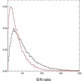
Figure 5: Normalized S/N distribution of VHJ detections for a 3 field strategy (black) and a 7 field strategy (red) assuming 1h blocks and 2 mmag RRN (model 4).

In the case of a 2 yr campaign the situation is the same. For all four planet populations it is more efficient to observe a higher number of fields (see Table 7). Therefore we conclude that observing 7 fields is the most efficient strategy and restrict our results in the following to 7 fields.

# fields	VHJ	HJ	WJ	VHS
3	7.73	5.52	1.60	2.26
4	9.82	6.97	1.95	2.63
5	12.06	8.43	2.44	3.05
6	14.00	9.41	2.61	3.40
7	15.76	10.28	2.78	3.51

Table 6: Number of planets found in the first year depending on the number of target fields, assuming 1h blocks and 2 mmag RRN (model 4).

# fields	VHJ	HJ	WJ	VHS
3	11.16	11.90	4.85	3.95
4	14.72	15.21	6.18	5.07
5	17.96	18.34	7.46	5.94
6	21.25	21.22	8.66	6.68
7	24.13	23.55	9.48	7.49

Table 7: Number of planets found in 2 yr depending on the number of target fields, assuming 1h blocks and 2 mmag RRN (model 4).

4.4 The expected number of planets in the Pan-Planets survey

In the previous sections we have identified our preferred survey strategy with 1h blocks and alternating among 7 fields. In addition we selected RRN model 4 as our preferred one. For these parameters we performed more detailed simulations in order to calculate the expected number of detections of the Pan-Planets project (including error estimates) and to study the parameter distributions of the detected planets in detail. For each of 4 different RRN levels (1 mmag, 2 mmag, 3 mmag and 4 mmag) and 4 planet populations (VHJ, HJ, WJ and VHS) we performed 25 000 simulation runs. The number of detections depending on the level of RRN are shown in Table 8. Fig. 6 shows the cumulative distribution of the host star brightness for each planet populations for 2 mmag of RRN (model 4).
Our predicted numbers are affected by two sources of uncertainties. The first and dominant one is the uncertainty of the planet frequency taken from Gould et al. (2006) which is caused by the low number statistics of the OGLE detections. This uncertainty is not included in Table 8 and must be taken into account by scaling all of our HJ results by a factor of $1^{+1.37}_{-0.59}$ and all of our VHJ results by a factor of $1^{+1.10}_{-0.54}$, as published in Gould et al. (2006).
The second uncertainty is a direct result of our simulations. Each simulation run represents one possible outcome of 1 sq.deg. of the Pan-Planets survey. Since the simulated observational epochs change from one run to the other and since in each run different stars are attributed to planets with different orbital parameters, an intrinsic scatter in the number of planets in found in each run. The combination of 49 randomly chosen runs represents one possible outcome of the full 49 sq.deg. survey (7 fields). From the histogram of these combinations we derive 68% confidence intervals for our predicted numbers.

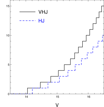
Figure 6: Cumulative host star brightness distributions for each planet population for a 1 yr campaign with 2 mmag RRN (model 4).

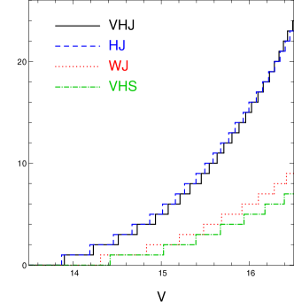
Figure 7: Cumulative host star brightness distributions for each planet population for a 2 yr campaign with 2 mmag RRN (model 4).

RRN level	VHJ	HJ	WJ	VHS
1 mmag	$18.4\pm 4.3$	$13.2\pm 3.7$	$3.8\pm 2.0$	$5.2\pm 2.3$
2 mmag	$15.8\pm 4.0$	$10.3\pm 3.2$	$2.8\pm 1.7$	$3.5\pm 1.9$
3 mmag	$11.7\pm 3.5$	$6.9\pm 2.7$	$1.8^{+1.4}_{-1.3}$	$1.9\pm 1.4$
4 mmag	$8.4\pm 2.9$	$4.5\pm 2.1$	$1.1^{+1.1}_{-0.9}$	$0.9^{+1.0}_{-0.7}$

Table 8: Number of planets found in the first year for our selected survey strategy as a function of residual red noise level (model 4).

4.5 Number of expected planets in a two year campaign

The Pan-Planets project has a lifetime of 3.5 years. In the previous sections we focus mainly on the first year of the survey. In this section we show the results of our simulations for a 2 year campaign. In particular, we address the question whether the project is more efficient if we stay on the same fields or if we choose new targets assuming that we find fields with similar densities (see §6).
Table 9 shows the number of planets detected in a 2 yr campaign for four different levels of RRN. Except for VHJ, we more than double the number of detections for each planet population. For the longer period WJ the gain is a factor of 3. In a 1 yr campaign most of these planets show less than 3 transits and are not detected. Adding the observations of the second year, the number of transits increases and many of the previously undetected planets are found.
In addition, staying on the same fields in the second year increases the S/N of all transit light curves, due to the higher number of data points taken during a transit. Planets that have an insufficiently high S/N after the first year are detected after the second year. This is particularly true for VHS.
Fig. 8 shows the fraction of all transiting Jupiter-sized planets (VHJ, HJ, WJ) that are detected in the first year of the survey (lower black line) and in the 2 yr campaign (upper red line). In the first year, the average efficiencies are 26.3%, 10.6% and 4.3% for VHJ, HJ and WJ respectively. Planets that have been missed do not have the required S/N, show less than 3 transits in the light curve, or the BLS algorithm found a wrong period. Extending the survey to the second year increases the efficiency significantly to 39.8%, 24.0% and 14.3% for VHJ, HJ and WJ respectively.

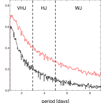
Figure 8: Fraction of all transiting VHJ, HJ and WJ that are detected as a function of period for a 1 yr campaign (lower black line) and a 2 yr campaign (upper red line).

RRN level	VHJ	HJ	WJ	VHS
1 mmag	28.1 $\pm$ 5.3	29.3 $\pm$ 5.4	12.4 $\pm$ 3.5	10.6 $\pm$ 3.3
2 mmag	24.1 $\pm$ 4.9	23.6 $\pm$ 4.9	9.5 $\pm$ 3.1	7.5 $\pm$ 2.7
3 mmag	19.0 $\pm$ 4.4	16.5 $\pm$ 4.1	6.1 $\pm$ 2.5	4.0 $\pm$ 2.1
4 mmag	14.4 $\pm$ 3.8	10.9 $\pm$ 3.3	4.0 $\pm$ 2.0	2.1 $\pm$ 1.5

Table 9: Number of planets found with 160h hours of observations in 2 yrs for our selected survey strategy as a function of residual red noise level (model 4).

4.6 The detection of Very Hot Neptunes

In this section we study the potential to find Very Hot Neptunes transiting M dwarfs. The radius ratio between planet and star is much higher for low mass stars which results in much deeper transits and therefore a higher detection probability. According to the Besançon model there are a total of 34 000 M dwarfs brighter than AB-magnitude $m_{i^{\prime}}$ = 18 mag in 7 fields of 7 sq.deg. each. These objects are particularly interesting, since the composition of planets in this mass range is rather unknown (gaseous, icy or rocky). Also the habitable zone is much closer to the star due to its lower surface temperature. Note, that only one planet transiting an M dwarf has been detected so far.
We consider all transiting VHN candidates down to host star brightnesses of $m_{i^{\prime}}$ = 18 mag to be interesting objects, although the spectroscopical follow-up will be very challenging. New high resolution near infrared spectrographs will help to confirm these very red objects.
To study the potential of Pan-Planets to find transiting VHN we perform simulations for the whole input stellar distribution and analyze the spectral type distribution of the hosts stars of all successful detections (Fig. 9). The Pan-Planets survey is sensitive to close-in Neptune-sized planets around late K and early M dwarfs if the frequency of these stars hosting Neptunes is as large as 5%. The number of VHN detections after the first and the second year is listed in Table 10 for 4 different residual rednoise levels. Assuming 2 mmag of RRN we expect to find 3 VHN after the first and 9 VHN after the second year.
Further we analyze the distance distributions of all detected VHJ, VHS and VHN systems (Fig. 10). The volume probed strongly depends on the radius of the planet. For lower mass radius the transit depth is generally smaller and therefore the photometric precision needed to detect the transits must be higher, which is only the case for closer and thus brighter systems. Note that for HJ and WJ the distance distributions are very similar to the VHJ distribution.

RRN level	1 yr	2 yr
1 mmag	$5.7\pm 2.4$	$16.6\pm 4.1$
2 mmag	$3.5\pm 1.9$	$9.7\pm 3.1$
3 mmag	$2.4\pm 1.6$	$6.3\pm 2.5$
4 mmag	$1.7\pm 1.4$	$4.6\pm 2.2$

Table 10: Number of VHN detections after the first and second year of the Pan-Planets survey for our selected survey strategy for different residual red noise levels (model 4).

Figure 9: Host star spectral type distribution of all detected VHN for a 2 yr campaign with 2 mmag RRN (model 4). Pan-Planets is sensitive to VHN transiting late K and early M dwarfs.

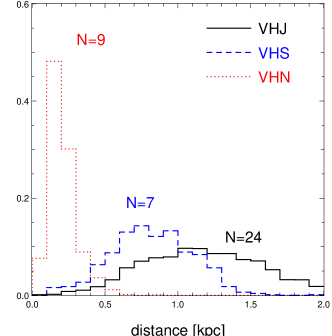
Figure 10: Distance distribution of the detected VHJ, VHS and VHN for a 2 yr campaign with 2 mmag RRN (model 4). Due to the lower transit depth smaller planets can only be detected around closer stars.

5 Consistency check with the OGLE-III survey

Gould et al. (2006) have modeled the OGLE-III survey in order to derive absolute frequencies of HJ and VHJ. In our simulations we are using these frequencies to predict the number of detections for the Pan-Planets survey. In order to verify our results we performed a consistency check by modeling the OGLE-III survey and comparing the results to the actual number of planets found. We limit this test to the 3 Carina fields where 3 planets have been found (1 HJ, 2 VHJ). The 2 bulge fields that have also been observed during the OGLE-III campaign are more difficult to model due to a stronger blending and a higher uncertainty in the input stellar distribution.
We obtained the Besançon model population of the 3 Carina fields (CAR100, CAR104, CAR105) for stars in the magnitude range of 13.7 $\leq I_{mag}\leq$ 17.0. The overall noise level as a function of magnitude has been determined by Gould et al. (2006) to be :

$$\sigma=-0.723+0.1544\cdot I_{mag}-0.01094\cdot I_{mag}^{2}+0.000259\cdot I_{mag}^{3}.$$ (6)

In their simulations Gould et al. (2006) did not include correlated noise sources, instead they account for systematics by using an increased S/N cut. In order to be as consistent as possible we follow the same procedure and do not split the over-all noise in red and white noise components (as we did in the Pan-Planets simulations). We use the radius and period distributions for HJ and VHJ introduced in §3.2. The epochs of the observations were taken from the light curve of OGLE-TR-74 with 1,200 epochs taken from February to May 2002.
After simulating the light curves in the same way as described in §3 we run the BLS algorithm and check for a correct period recovery. In addition we apply the following cuts which have been used by the OGLE group and are summarized in detail in Section 3 and Table 1 in Gould et al. (2006): the transit depth $\delta$ must be smaller than 0.04 mag ($\sim$3.62%); the S/N greater than 11.6; the signal detection efficiency larger than 3.8; the number of transits is required to be at least 3; and finally, the color $(V-I)_{0}$ must be greater than 0.4. Note that we have not imposed any cut on the transit depth in our simulations for the Pan-Planets survey since a Jupiter-sized planet transiting an M dwarf can have a fairly high transit depth. Further we do not use a color since in our simulations we include only late type dwarfs a priori.
In total we simulated 50 000 runs for each of the five planet populations. On average we find 2.18 VHJ and 1.46 HJ which is in reasonable good agreement with the actual number of 2 VHJ and 1 HJ found by the OGLE group.
According to our simulations the OGLE-III carina survey was not sensitive to one of the other 3 planet populations we tested. We find on average 0.45 WJ, 0.12 VHS and zero VHN which is agreement with none being found by OGLE.

6 Conclusion

The aim of this work was to study the influence of the survey strategy on the efficiency of the Pan-Planets project and to predict the number of detections for an optimized strategy.
Our calculations are based on the simulation of realistic light curves including the effects of limb-darkening, ingress/egress and observational window functions. In addition we have introduced a model to simulate correlated (red) noise which allows us to include the effects of correlated noise on the efficiency of the BLS detection algorithm. Our approach can be applied to any transit survey as well.

Below we summarize the caveats and assumptions that were made in our simulations :

• Our results depend on the spectral type and magnitude distribution of the Besançon model. The model does not include second order substructure such as spiral arms.

• We neglect the effects of blending. Due to crowding into the direction of the Galactic disk some stars are blended by neighboring sources.

• We assume all planets that are detected by the BLS-algorithm to be followed-up and confirmed spectroscopically. In particular, we assume that no true candidate is rejected by any candidate selection process. The detailed follow-up strategy of the Pan-Planets survey will be presented in Afonso et al. (in prep.).

• Our simulations are done for 1 sq.deg. and the results are scaled to the actual survey area. We assume that all fields (3, 4, 5, 6 or 7 case) have homogeneous densities and non-varying (or similar) stellar populations. Simple number counts on the USNO-catalog showed that we can find up to 7 fields with similar total number of stars (see §4). For a larger number of fields, the assumption of a constant density might be too optimistic since we are restricted to fields that are close to each other in order to keep the observational overhead low.

• Our results directly scale with the assumed planet frequencies. The values of 0.14% and 0.31% we use for VHJ and HJ have uncertainties of a factor of 2. For WJ, VHS and VHN we have used hypothetical values of 0.31%, 0.14% and 5% respectively. After completion of the Pan-Planets survey we will be able to derive more accurate absolute frequencies for all five planet populations.

• The quality of the data is assumed to be homogeneously good over the whole detector area. Bad pixel regions and gaps between the individual CCDs are not taken into account and result in an effective field of view that is smaller than 7 sq.deg.

Comparing different observing strategies we found that observing more fields is more efficient. Concerning the observation time per night, we compared 1h blocks to 3h blocks and found the shorter ones to be more efficient. This is still the case for a 2 yr campaign.

For an RRN level of 2 mmag we expect to find up to 15 VHJ and 10 HJ in the first year around stars brighter than V = 16.5 mag. The survey will also be sensitive to planets with longer periods (WJ) and smaller radii (VHS and VHN). Assuming that the frequencies of stars with WJ and VHS is 0.31% and 0.14% respectively, we expect to find up to 2 WJ and 3 VHS in the same magnitude range.
We found that observing the same fields in the second year of the 3.5 yr lifetime of the survey is more efficient than choosing new fields. We expect to find up to 24 VHJ, 23 HJ, 9 WJ and 7 VHS. In particular for longer periods (HJ and WJ) and smaller radii (VHS) we will more than double the number of detections of the first year if we continue to observe the same targets.
We have investigated the potential of the Pan-Planets survey to detect VHN transiting M dwarfs brighter than i’ = 18 mag. Assuming the frequency of these objects is 5%, we expect to find up to 3 detections in the first year and up to 9 detections observing the same fields in the second year.
As a consistency check we modeled the OGLE-III Carina survey and found 2.18 VHJ, 1.46 HJ, 0.45 WJ, 0.12 VHS and zero VHN which is in agreement with the 2 VHJ and 1 HJ and the zero WJ, VHS and VHN that have been actually detected.