Achievable Rates and Training Optimization for Fading Relay Channels with Memory

Abstract

In this paper, transmission over time-selective, flat fading relay channels is studied. It is assumed that channel fading coefficients are not known a priori. Transmission takes place in two phases: network training phase and data transmission phase. In the training phase, pilot symbols are sent and the receivers employ single-pilot MMSE estimation or noncausal Wiener filter to learn the channel. Amplify-and-Forward (AF) and Decode-and-Forward (DF) techniques are considered in the data transmission phase and achievable rate expressions are obtained. The training period, and data and training power allocations are jointly optimized by using the achievable rate expressions. Numerical results are obtained considering Gauss-Markov and lowpass fading models. Achievable rates are computed and energy-per-bit requirements are investigated. The optimal power distributions among pilot and data symbols are provided.

I Introduction

In wireless communications, channel conditions vary randomly over time due to mobility and changing environment. If the channel conditions are not known a priori, practical wireless systems generally employ pilot symbols to learn the channel. In one of the early studies in this area, Cavers provided an analytical approach to the design of pilot-assisted transmissions in [1] and [2]. Considering adaptive coding of data symbols without feedback to the transmitter, Abou-Faycal et al. [4] studied the data rates achieved with pilot-symbol-assisted modulation (PSAM) over Gauss-Markov fading channels. The authors in [6] also studied the PSAM over Gauss-Markov channels and analyzed the power allocated to the data symbols when the pilot symbol has fixed power. They showed that the power of a data symbol decreases as its distance to the pilot symbol increases.

Recently, cooperative wireless communications has attracted much interest. Cooperative relay transmission techniques have been studied in [8] and [9] where Amplify-and-Forward (AF) and Decode-and-Forward (DF) models are considered. However, most of the studies have assumed that the channel conditions are perfectly known at the receiver and/or transmitter. In one of the recent studies, Wang et al. [7] considered wireless sensory relay networks where the conditions of the channels are learnt imperfectly only by the relay nodes.

In this paper, we study the training-based transmission and reception schemes over a priori unknown, Rayleigh fading relay channels in which the fading is modeled as a random process with memory. Unknown fading coefficients of the channels are estimated at the receivers with the assistance of the pilot symbols. We consider two channel estimation methods: single-pilot minimum mean-square-error (MMSE) estimation and noncausal Wiener filter estimation. We study AF and DF relaying techniques with two different transmission protocols. We obtain achievable rate expressions and optimize the training parameters by maximizing these expressions. We concentrate on the Gauss-Markov and lowpass fading processes for numerical analysis.

II Channel Model

We consider a three-node-relay network which consists of one source node, one relay node and one destination node. Source-destination, source-relay and relay-destination channels are modeled as Rayleigh fading channels with fading coefficients denoted by $h_{sd}\sim\mathcal{CN}(0,\sigma_{sd}^{2})$, $h_{sr}\sim\mathcal{CN}(0,\sigma_{sr}^{2})$ and $h_{rd}\sim\mathcal{CN}(0,\sigma_{rd}^{2})$, respectively. Each channel is independent of others and exhibits memory with an arbitrary correlation structure. Hence $\{h_{sd}\}$, $\{h_{sr}\}$, and $\{h_{rd}\}$ are assumed to be mutually independent Gaussian random processes with power spectral densities $S_{h_{sd}}(e^{jw})$, $S_{h_{sr}}(e^{jw})$ and $S_{h_{rd}}(e^{jw})$, respectively. In this relay network, information is sent from the source to the destination with the aid of the relay. Transmission takes place in two phases: network training phase and data transmission phase. Over a duration of $M$ symbols, the source and the relay are subject to the following power constraints:

$$\|\textbf{x}_{s,t}\|^{2}+E\{\|\textbf{x}_{s}\|^{2}\}\leq MP_{s}$$ (1)

$$\|\textbf{x}_{r,t}\|^{2}++E\{\|\textbf{x}_{r}\|^{2}\}\leq MP_{r}$$ (2)

where $\textbf{x}_{s,t}$ and $\textbf{x}_{r,t}$ are the source and relay pilot vectors, respectively, and $\textbf{x}_{s}$ and $\textbf{x}_{r}$ are the data vectors sent by the source and the relay, respectively.

III Network Training Phase

In the network training phase, source and relay send pilot symbols in nonoverlapping intervals with a period of $M$ symbols to facilitate channel estimation at the receivers. In a block of $M$ symbols, transmission takes place in the following order. First, the source sends a single pilot symbol $x_{s,t}$, and the relay and destination receives

$$y_{r,t}=h_{sr}x_{s,t}+n_{r}\quad\text{and}\quad y_{d,t}=h_{sd}x_{s,t}+n_{d},$$ (3)

and estimates $h_{sr}$ and $h_{sd}$, respectively. Then, transmission enters the data transmission phase, and source sends an $(M-2)/2$-dimensional data vector that is again received by the relay and destination terminals. Next, only the relay sends a single pilot symbol $x_{r,t}$, and the signal received at the destination node is

$$y_{d,t}^{r}=h_{rd}x_{r,t}+n_{d}^{r},$$ (4)

which is used by the destination to estimate $h_{rd}$. In (3) and (4), $n_{r}$, $n_{d}$, and $n_{d}^{r}$ are assumed to be independent and identically distributed (i.i.d.) zero mean Gaussian random variables with variance $\sigma_{n}^{2}$, modeling the additive thermal noise present at the receivers. In the remaining duration of $(M-2)/2$ symbols, transmission again enters the data transmission phase. In this case, the relay transmits an $(M-2)/2$ dimensional data vector to the destination while the source either becomes silent or continues its transmission depending on the cooperation protocol. This order of transmission is repeated for the next block of $M$ symbols.

As noted before, we consider two channel estimation methods. In the first method, only a single pilot symbol is used to obtain the MMSE estimate of the channel fading coefficients. As described in [5], MMSE estimates of the fading coefficients and the variances of the estimate errors are given as follows:

$$\widehat{h}_{sr}=\frac{\sigma_{sr}^{2}\sqrt{P_{x_{s,t}}}}{\sigma_{sr}^{2}P_{x_{s,t}}+\sigma_{n}^{2}}y_{r,t},\quad\sigma_{\widetilde{h}_{sr}}^{2}=\frac{\sigma_{sr}^{2}\sigma_{n}^{2}}{\sigma_{sr}^{2}P_{x_{s,t}}+\sigma_{n}^{2}}$$ (5)

$$\widehat{h}_{sd}=\frac{\sigma_{sd}^{2}\sqrt{P_{x_{s,t}}}}{\sigma_{sd}^{2}P_{x_{s,t}}+\sigma_{n}^{2}}y_{d,t},\quad\sigma_{\widetilde{h}_{sd}}^{2}=\frac{\sigma_{sd}^{2}\sigma_{n}^{2}}{\sigma_{sd}^{2}P_{x_{s,t}}+\sigma_{n}^{2}}$$ (6)

$$\widehat{h}_{rd}=\frac{\sigma_{rd}^{2}\sqrt{P_{x_{r,t}}}}{\sigma_{rd}^{2}P_{x_{r,t}}+\sigma_{n}^{2}}y_{d,t}^{r},\quad\sigma_{\widetilde{h}_{rd}}^{2}=\frac{\sigma_{rd}^{2}\,\sigma_{n}^{2}}{\sigma_{rd}^{2}P_{x_{s,t}}+\sigma_{n}^{2}}$$ (7)

where $P_{x_{s,t}}$ and $P_{x_{r,t}}$ are the power of the pilot symbols sent by the source and the relay, respectively, and $y_{r,t}\sim\mathcal{CN}(0,\sigma_{sr}^{2}P_{x_{s,t}}+\sigma_{n}^{2})$, $y_{d,t}\sim\mathcal{CN}(0,\sigma_{sd}^{2}P_{x_{s,t}}+\sigma_{n}^{2})$ and $y_{d,t}^{r}\sim\mathcal{CN}(0,\sigma_{rd}^{2}P_{x_{r,t}}+\sigma_{n}^{2})$.

In the second method, we employ the noncausal Wiener filter which is the optimum linear estimator in the mean-square sense. The Wiener filter is employed at both the relay and the destination. Note that since pilot symbols are sent with a period of $M$ symbols, the channels are sampled every $MT_{s}$ seconds, where $T_{s}$ is the sampling time. As described in [10], we have to consider the undersampled versions of the Doppler spectrums of the fading coefficients, which are given by

$$S_{h_{sr},m}(e^{jw})=\frac{1}{M}\sum_{k=0}^{M-1}e^{jm(w-2\pi k)/M}S_{h_{sr}}\left(e^{j(w-2\pi k)/M}\right)$$ (8)

$$S_{h_{sd},m}(e^{jw})=\frac{1}{M}\sum_{k=0}^{M-1}e^{jm(w-2\pi k)/M}S_{h_{sd}}\left(e^{j(w-2\pi k)/M}\right)$$ (9)

$$S_{h_{rd},m}(e^{jw})=\frac{1}{M}\sum_{k=0}^{M-1}e^{jm(w-2\pi k)/M}S_{h_{rd}}\left(e^{j(w-2\pi k)/M}\right).$$ (10)

Then, the channel MMSE variances for the noncausal Wiener filter at time $Ml+m$ are given by [11]

$$\sigma_{\widetilde{h}_{sr}}^{2}(Ml+m)=\sigma_{sr}^{2}-\frac{1}{2\pi}\int_{-\pi}^{\pi}\frac{P_{x_{s,t}}|S_{h_{sr},m}(e^{jw})|^{2}}{P_{x_{s,t}}S_{h_{sr},0}(e^{jw})+\sigma_{n}^{2}}dw$$ (11)

$$\sigma_{\widetilde{h}_{sd}}^{2}(Ml+m)=\sigma_{sd}^{2}-\frac{1}{2\pi}\int_{-\pi}^{\pi}\frac{P_{x_{s,t}}|S_{h_{sd},m}(e^{jw})|^{2}}{P_{x_{s,t}}S_{h_{sd},0}(e^{jw})+\sigma_{n}^{2}}dw$$ (12)

$$\sigma_{\widetilde{h}_{rd}}^{2}(Ml+m)=\sigma_{rd}^{2}-\frac{1}{2\pi}\int_{-\pi}^{\pi}\frac{P_{x_{r,t}}|S_{h_{rd},m}(e^{jw})|^{2}}{P_{x_{r,t}}S_{h_{rd},0}(e^{jw})+\sigma_{n}^{2}}dw$$ (13)

$$\text{for }\quad l=0,1,2,\ldots\quad\text{and}\quad m=0,1\dots(M-1).$$

After obtaining the estimates, we can express the fading coefficients as

$$h_{sr}(Ml+m)=\widehat{h}_{sr}(Ml+m)+\widetilde{h}_{sr}(Ml+m)$$

$$h_{sd}(Ml+m)=\widehat{h}_{sd}(Ml+m)+\widetilde{h}_{sd}(Ml+m)$$

$$h_{rd}(Ml+m)=\widehat{h}_{rd}(Ml+m)+\widetilde{h}_{rd}(Ml+m).$$ (14)

IV Data Transmission Phase

Note that as described in the previous section, within a block of $M$ symbols, two symbol durations are allocated for channel training while data transmission is performed in the remaining portion of the time. We assume that relay operates in half-duplex mode. Hence, the relay first listens and then transmits to the destination. We consider two transmission protocols: non-overlapped and overlapped transmissions.

IV-A Non-overlapped Case

In this protocol, the source and relay send data symbols in nonoverlapping intervals. The source, after sending the pilot symbol, sends its $(M-2)/2$ data symbols which are received by the relay and the destination as

$$y_{r,d}(m)=h_{sr}(m)x_{s,d}(m)+n_{r}(m)$$ (15)

$$y_{d,d}(m)=h_{sd}(m)x_{s,d}(m)+n_{d}(m)\quad m=2,\ldots\frac{M}{2}.$$

Next, the source stops transmission, and the relay sends first its pilot symbol and then $(M-2)/2$ data symbols which are generated from $\textbf{y}_{r,d}=[y_{r,d}(2),\ldots,y_{r,d}(M/2)]$. Thus the destination receives

$$y_{d,d}(j)=h_{rd}(j)x_{r,d}(j)+n_{d}(j)\quad j=m+M/2$$ (16)

where again $m=2,\ldots,M/2$. After substituting (III) into (15) and (16), we obtain

$$y_{r,d}(m)=\widehat{h}_{sr}(m)x_{s,d}(m)+\widetilde{h}_{sr}(m)x_{s,d}(m)+n_{r}(m)$$ (17)

$$y_{d,d}(m)=\widehat{h}_{sd}(m)x_{s,d}(m)+\widetilde{h}_{sd}(m)x_{s,d}(m)+n_{d}(m)$$

$$y_{d,d}(j)=\widehat{h}_{rd}(j)x_{r,d}(j)+\widetilde{h}_{rd}(j)x_{r,d}(j)+n_{d}(j)$$

where $m=2,\ldots,M/2$ and $j=m+M/2$.

IV-B Overlapped Case

In this protocol, the source continues its transmission while the relay is sending its data symbols. The source becomes silent only when the relay is sending the pilot symbol. Therefore, the received signals in the data transmission phase can be written as

$$y_{r,d}(m)=h_{sr}(m)x_{s,d}(m)+n_{r}(m)$$ (18)

$$y_{d,d}(m)=h_{sd}(m)x_{s,d}(m)+n_{d}(m)$$

$$y_{d,d}(j)=h_{sd}(j)x_{s,d}(j)+h_{rd}(j)x_{r,d}(j)+n_{d}(j)$$

where $m=2,...,M/2$ and $j=m+M/2$. Similarly as in the non-overlapped case, we can integrate the estimation results to (18) and write

$$y_{r,d}(m)=\widehat{h}_{sr}(m)x_{s,d}(m)+\widetilde{h}_{sr}(m)x_{s,d}(m)+n_{r}(m)$$ (19)

$$y_{d,d}(m)=\widehat{h}_{sd}(m)x_{s,d}(m)+\widetilde{h}_{sd}(m)x_{s,d}(m)+n_{d}(m)$$

$$y_{d,d}(j)=\widehat{h}_{sd}(j)x_{s,d}(j)+\widetilde{h}_{sd}(j)x_{s,d}(j)$$

$$+\widehat{h}_{rd}(j)x_{r,d}(j)+\widetilde{h}_{rd}(j)x_{r,d}(j)+n_{d}(j).$$

V Achievable Rates for AF Scheme

In this section, we consider the AF relaying scheme in which the relay sends to the destination simply the scaled version of the signal received from the source. An achievable rate expression for the AF scheme is obtained by maximizing the mutual information between the transmitted signal vector $\textbf{x}_{s,d}$ and the $(M\!\!\!-\!\!\!2)$-dimensional received signal $\textbf{y}_{d,d}=[y_{d,d}(2),\ldots,y_{d,d}(M/2),y_{d,d}(M/2+2),\ldots,y_{d,d}(M)]$ given the estimates of the fading coefficients. $\widehat{\textbf{h}}_{sr}$, $\widehat{\textbf{h}}_{sd}$ and $\widehat{\textbf{h}}_{rd}$ are used to denote the vectors of channel estimates. Therefore, an achievable rate expression is given by

$$I_{AF}=\sup_{p_{\textbf{x}_{s}}}\frac{1}{M}\textit{I}(\textbf{x}_{s,d};\textbf{y}_{d,d}|\widehat{\textbf{h}}_{sr},\widehat{\textbf{h}}_{sd},\widehat{\textbf{h}}_{rd}).$$ (20)

Note that the above formulation supposes that the destination node also knows $\widehat{\textbf{h}}_{sr}$. Hence, it is assumed that these estimates are reliably forwarded by the relay to the destination using low rate links. A lower bound on $I_{AF}$ can be obtained by assuming similarly as in [3] that the estimation errors are additional sources of worst-case Gaussian noise. We define the new noise random variables in non-overlapped and overlapped cases as

$$z_{r,d}(m)=\widetilde{h}_{sr}(m)x_{s,d}(m)+n_{r}(m)$$ (21)

$$z_{d,d}(m)=\widetilde{h}_{sd}(m)x_{s,d}(m)+n_{d}(m)$$

$$z_{d,d}(j)=\widetilde{h}_{rd}(j)x_{r,d}(j)+n_{d}(j)$$

and

$$z_{r,d}(m)=\widetilde{h}_{sr}(m)x_{s,d}(m)+n_{r}(m)$$ (22)

$$z_{d,d}(m)=\widetilde{h}_{sd}(m)x_{s,d}(m)+n_{d}(m)$$

$$z_{d,d}(j)=\widetilde{h}_{sd}(j)x_{s,d}(j)+\widetilde{h}_{rd}(j)x_{r,d}(j)+n_{d}(j)$$

respectively. By assuming that the new noise components are Gaussian random variables and using techniques similar to those in [12], we can obtain the following worst-case achievable rate expression for the non-overlapped case:

$$I_{nonover}=\frac{1}{M}E_{w_{sr}}E_{w_{sd}}E_{w_{rd}}\sum_{m=2}^{M/2}\log\left(1+a_{1,m}+f(b_{1,m},c_{1,j})\right)$$ (23)

where

$$a_{1,m}=\frac{P_{x_{s,d}(m)}\sigma_{\widehat{h}_{sd}(m)}^{2}}{\sigma_{z_{d,d}(m)}^{2}}|w_{sd}|^{2},\quad b_{1,m}=\frac{P_{x_{s,d}(m)}\sigma_{\widehat{h}_{sr}(m)}^{2}}{\sigma_{z_{r,d}(m)}^{2}}|w_{sr}|^{2},$$ (24)

$$c_{1,j}=\frac{P_{x_{r,d}(j)}\sigma_{\widehat{h}_{rd}(j)}^{2}}{\sigma_{z_{d,d}(j)}^{2}}|w_{rd}|^{2},\quad f(x,y)=\frac{xy}{1+x+y}$$

and $w_{sd}\sim\mathcal{CN}(0,1)$, $w_{sr}\sim\mathcal{CN}(0,1)$, $w_{rd}\sim\mathcal{CN}(0,1)$. $P_{x_{s,d}(m)}$ and $P_{x_{r,d}(j)}$ are the powers of the $m^{th}$ source symbol and $j^{th}$ relay symbol, respectively, and $\sigma_{\widehat{h}_{sr}(m)}^{2}=\sigma_{sr}^{2}-\sigma_{\widetilde{h}_{sr}(m)}^{2}$, $\sigma_{\widehat{h}_{sd}(m)}^{2}=\sigma_{sd}^{2}-\sigma_{\widetilde{h}_{sd}(m)}^{2}$, $\sigma_{\widehat{h}_{rd}(m)}^{2}=\sigma_{rd}^{2}-\sigma_{\widetilde{h}_{rd}(m)}^{2}$. Finally, note that $j=m+M/2$.

Similarly, we can find the following achievable rate expression for the overlapped case:

$$I_{over} =\frac{1}{M}E_{w_{sr}}E_{w_{sd}}E_{w_{rd}}$$ (25)

$$\sum_{m=2}^{M/2}\log\left(1+a_{2,m}+f(d_{2,m},c_{2,j})+q(a_{2,m},b_{2,j},c_{2,j},d_{2,m})\right)$$

where

$$a_{2,m}=\frac{P_{x_{s,d}(m)}\sigma_{\widehat{h}_{sd}(m)}^{2}}{\sigma_{z_{d,d}(m)}^{2}}|w_{sd}|^{2},b_{2,j}=\frac{P_{x_{s,d}(j)}\sigma_{\widehat{h}_{sd}(j)}^{2}}{\sigma_{z_{d,d}(j)}^{2}}|w_{sd}|^{2},$$ (26)

$$c_{2,j}=\frac{P_{x_{r,d}(j)}\sigma_{\widehat{h}_{rd}(j)}^{2}}{\sigma_{z_{d,d}(j)}^{2}}|w_{rd}|^{2},d_{2,m}=\frac{P_{x_{s,d}(m)}\sigma_{\widehat{h}_{sr}(m)}^{2}}{\sigma_{z_{r,d}(m)}^{2}}|w_{sr}|^{2}$$

and $q(a,b,c,d)=\frac{(1+a)b(1+c)}{1+c+d}\quad\text{and}\quad j=m+M/2.$

VI Achievable Rates for DF Scheme

The repetition coding and the parallel coding are two possible coding techniques used in DF schemes [8]. First, we consider the repetition coding, and for this case the achievable rate is given by

$$I_{rc}=\frac{1}{M}\sup_{p_{\textbf{x}_{s}}}\left\{\min\left[\textit{I}(\textbf{x}_{s,d};\textbf{y}_{r,d}|\widehat{\textbf{h}}_{sr}),\textit{I}(\textbf{x}_{s,d};\textbf{y}_{d,d}|\widehat{\textbf{h}}_{sd},\widehat{\textbf{h}}_{rd})\right]\right\}$$ (27)

Employing the techniques used in the AF non-overlapped scheme, we obtain the following achievable rate expression for non-overlapped DF with repetition coding:

$$I_{nonover,rc}=\frac{1}{M}E_{w_{sr}}E_{w_{sd}}E_{w_{rd}}\sum_{m}\min(I_{1},I_{2})$$ (28)

where

$$I_{1}=\log\left[1+b_{1,m}\right],\quad I_{2}=\log\left[1+a_{1,m}+c_{1,j}\right],$$

and $a_{1,m},b_{1,m}$ and $c_{1,j}$ are given in (24). For the overlapped case of the DF repetition coding, (28) holds with $I_{1}$ and $I_{2}$ defined as

$$I_{1}=\log\left[1+c_{2,j}\right],\quad I_{2}=\log\left[1+a_{2,m}+b_{2,j}+d_{2,m}+a_{2,m}b_{2,j}\right]$$

where $a_{2,m},b_{2,j},c_{2,j},$ and $d_{2,m}$ are given in (26). When we employ the parallel coding, we have

$$I_{pc}=\frac{1}{M}\sup_{P_{\textbf{x}_{s}},P_{\textbf{x}_{r}}}$$ (29)

$$\left\{\min\left[\textit{I}(\textbf{x}_{s,d};\textbf{y}_{r,d}|\widehat{\textbf{h}}_{sr}),\textit{I}(\textbf{x}_{s,d};\textbf{y}_{d,d}|\widehat{\textbf{h}}_{sd})+\textit{I}(\textbf{x}_{r,d};\textbf{y}_{d,d}|\widehat{\textbf{h}}_{rd})\right]\right\}.$$

Similarly, we can find, for the nonoverlapping case, an achievable rate expression given by

$$I_{nonover,pc}=\frac{1}{M}E_{w_{sr}}E_{w_{sd}}E_{w_{rd}}\sum_{m}\min(I_{1},I_{2})$$ (30)

where

$$I_{1}=\log(1+b_{1,m}),\quad I_{2}=\log(1+a_{1,m})+\log(1+c_{1,j}).$$

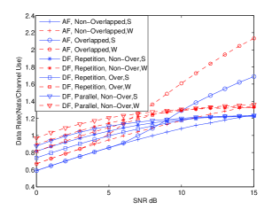
Figure 1: The optimal achievable rates vs. SNR for the Gauss-Markov fading model ($\alpha=0.99$) and different relaying techniques. $\sigma_{sd}^{2}=1,\sigma_{sr}^{2}=16$ and $\sigma_{rd}^{2}=16$. (S: single-pilot estimation. W: Wiener filter.)

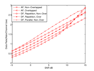
Figure 2: The optimal achievable rates vs. SNR for the lowpass fading model when noncausal Wiener filter is employed. $\sigma_{sd}^{2}=1,\sigma_{sr}^{2}=16$ and $\sigma_{rd}^{2}=16$.

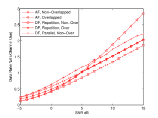
Figure 3: The optimal achievable rates vs. SNR for the lowpass fading model when noncausal Wiener filter is employed. $\sigma_{sd}^{2}=1,\sigma_{sr}^{2}=4$ and $\sigma_{rd}^{2}=4$.

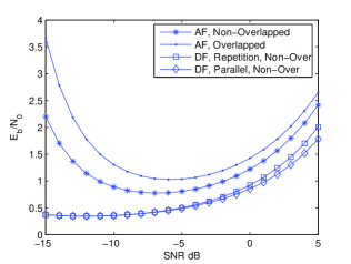
Figure 4: Normalized bit energies $\frac{E_{b}}{N_{0}}$ vs. SNR for the lowpass fading model when noncausal Wiener filter is employed. $\sigma_{sd}^{2}=1,\sigma_{sr}^{2}=16$ and $\sigma_{rd}^{2}=16$.

VII Optimizing Training Parameters

In this section, we consider two particular fading processes. In the first case, fading is modeled as a first-order Gauss-Markov process whose dynamics is described by

$$h_{k}=\alpha h_{k-1}+z_{k}\quad 0\leq\alpha\leq 1\quad k=1,2,3,\ldots$$

where {$z_{k}$} are i.i.d. circular complex Gaussian variables with zero mean and variance equal to (1-$\alpha^{2})\sigma_{h}^{2}$. In the above formulation, $\alpha$ is a parameter that controls the rate of the channel variations between consecutive transmissions. The power spectral density of the Gauss-Markov process with variance $\sigma_{h}^{2}$ is given by

$$S_{h}(e^{jw})=\frac{(1-\alpha^{2})\sigma_{h}^{2}}{1+\alpha^{2}-2\alpha\cos(w)}.$$ (31)

We also model the fading as a lowpass Gaussian process whose power spectral density is given by

$$S_{h}(e^{jw})=\left\{\begin{split}&\frac{\sigma_{h}^{2}}{2f_{d}},\quad&\text{for }|w|<w_{d}\\ &0,\quad&\text{otherwise}\end{split}\right.$$ (32)

where $w_{d}=2\pi f_{d}$ is the maximum Doppler spread in radians.

In Gauss-Markov channels, it is difficult to find a closed-form expression for the variance of the estimate error when Wiener filter is used, because the channel’s spectrum is not band limited. Therefore, there is always aliasing in the undersampled Doppler spectrums, which causes an increase in the variance of the error. On the other hand, when fading is modeled as a lowpass process, we can find a explicit solution for the error variance, and we can express it as

$$\sigma_{\widetilde{h}}^{2}=\frac{\sigma_{h}^{2}\sigma_{n}^{2}}{P_{x,t}\sigma_{h}^{2}+\sigma_{n}^{2}}.$$

In the lowpass case, if the channel is sampled sufficiently fast (i.e., $M<\frac{1}{2f_{d}}$), there is no aliasing and the power is distributed equally among data symbols. However, note that the power allocated to the data symbols of the source is not equal to the power allocated to the data symbols of the relay. In general, if there is aliasing or a single pilot is used for estimation, the power allocated to the data symbols will differ depending on their distance to the pilot signals.

Having obtained achievable rate expressions, our next goal is to jointly optimize training period $M$, training power, and power allocated to the data symbols.

VIII Numerical Results

In this section, we present numerical optimization results. In Figure 1, we plot the optimal achievable rates with respect to SNR for different relaying protocols by using two different methods of channel estimation. Fading is assumed to be a Gauss-Markov process. The dashed lines indicate the optimal data rates obtained when noncausal Wiener filter is used, whereas the solid lines show the optimal data rates obtained when a single pilot symbol is used for estimation. The rates are optimal in the sense that they are obtained with optimal training parameters and optimal power allocations. We can see that at low SNR values, DF provides higher rates and parallel non-overlapped DF scheme is the most efficient one. As expected, Wiener filter performance is better than that of the estimation that uses a single pilot. Moreover, at low SNR values non-overlapped and overlapped relaying schemes give the same optimal results, and optimal power distributions among data and pilot symbols are the same for both. On the other hand, at high SNR values, we see a significant increase in the data rate of AF overlapped scheme compared to the other schemes.

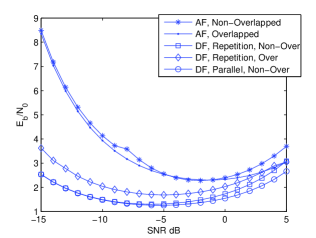
Figure 5: Normalized bit energies $\frac{E_{b}}{N_{0}}$ vs. SNR for the lowpass fading model when noncausal Wiener filter is employed. $\sigma_{sd}^{2}=1,\sigma_{sr}^{2}=4$ and $\sigma_{rd}^{2}=4$.

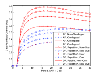
Figure 6: The optimal achievable rates vs. training period $M$ for the Gauss-Markov fading model. Single-pilot MMSE estimation is employed. The dashed lines are obtained when $\sigma_{sd}^{2}=1,\sigma_{sr}^{2}=4$ and $\sigma_{rd}^{2}=4$ and solid lines are obtained when $\sigma_{sd}^{2}=1,\sigma_{sr}^{2}=16$ and $\sigma_{rd}^{2}=16$

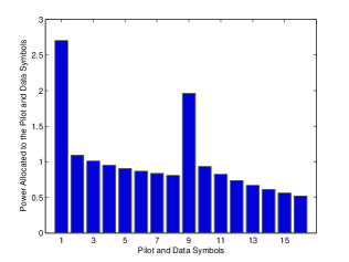
Figure 7: Optimal power distribution among the pilot and data symbols when $\sigma_{sd}^{2}=1,\sigma_{sr}^{2}=16$,$\sigma_{rd}^{2}=16$, SNR=0dB. Fading is a Gauss-Markov process with $\alpha=0.99$. Single-pilot MMSE estimation is employed. The optimal period is $M=16$. Note that the first 8 symbols belong to the source and the last 8 bars belong to the relay.

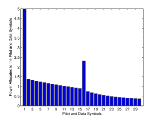
Figure 8: Optimal power distribution among the pilot and data symbols when $\sigma_{sd}^{2}=1,\sigma_{sr}^{2}=4$,$\sigma_{rd}^{2}=4$, SNR=0dB. Fading is a Gauss-Markov process with $\alpha=0.99$. Single-pilot MMSE estimation is employed. The optimal period is $M=30$. Note that the first 15 symbols belong to the source and the last 15 bars belong to the relay

In Fig. 2 and Fig. 3, we plot the optimal data rates when we estimate the lowpass fading process using a noncausal Wiener filter. The channel variances are $\sigma_{sd}^{2}=1,\sigma_{sr}^{2}=16,$ $\sigma_{rd}^{2}=16$, and $\sigma_{sd}^{2}=1,\sigma_{sr}^{2}=4$ and $\sigma_{rd}^{2}=4$, respectively. Conclusions similar to that given for Fig. 1 are drawn again. In Figs. 4 and 5, the bit energy normalized by the noise variance, $\frac{E_{b}}{N_{0}}$, is plotted as a function of SNR. In all cases, we observe that minimum bit energy is achieved at a nonzero SNR value. If SNR is further decreased, higher bit energy values are required and hence, operation at these very low SNRs should be avoided.

In Figure 6, we plot the optimal data rates as a function of the training period, $M$, when SNR=0 dB for different relaying schemes and different channel variances. Single-pilot-symbol estimation is employed. Since a relatively low SNR value is considered, AF non-overlapped and AF overlapped schemes provide lowest rates. The highest performance is obtained when DF parallel non-overlapped scheme is used.

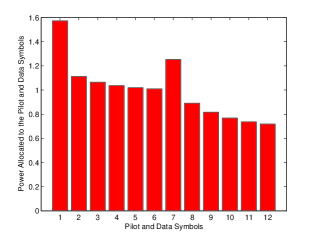
Figure 9: Optimal power distribution among the pilot and data symbols when $\sigma_{sd}^{2}=1,\sigma_{sr}^{2}=16$,$\sigma_{rd}^{2}=16$, SNR=0dB. Fading is a Gauss-Markov process with $\alpha=0.99$. Wiener filter is employed. The optimal period is $M=12$. Note that the first 6 symbols belong to the source and the last 6 bars belong to the relay

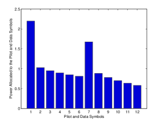
Figure 10: Optimal power distribution among the pilot and data symbols when $\sigma_{sd}^{2}=1,\sigma_{sr}^{2}=16$,$\sigma_{rd}^{2}=16$,SNR=0dB. Fading is a Gauss-markov process with $\alpha=0.99$. Single-pilot MMSE estimation is employed. The optimal period $M=12$. Note that the first 6 symbols belong to the source and the last 6 bars belong to the relay

In Figs. 7 and 8, power allocated to the pilot and data symbols is plotted when Gauss-Markov channel is considered and AF non-overlapped scheme is employed. The first half of the bars shows the power allocated to the source symbols and the rest shows the power allocated to the relay symbols. The first bar of the each group gives the power of the pilot symbols. Note that these power distributions are obtained when the period is at its optimal value when SNR=0 dB. The optimal periods are 16 and 30 when $\sigma_{sd}^{2}=1,\sigma_{sr}^{2}=16$, $\sigma_{rd}^{2}=16$, and $\sigma_{sd}^{2}=1,\sigma_{sr}^{2}=4$, $\sigma_{rd}^{2}=4$, respectively. In Figure 9, the optimal power distribution is displayed when noncausal Wiener filter is used for estimation at SNR = 0 dB. Note that the optimal period is 12. In Figure 10, we plot the power distribution when single-pilot estimation is performed at the optimal period 12 of Wiener Filter estimation. It is observed that more power is given to the pilot symbols when single-pilot-symbol estimation is used. However, when we employ noncausal Wiener filter, the power allocated to the pilot symbols is decreased thereby increasing the data rate by giving more power to the data symbols.

IX Conclusion

We have studied transmission over imperfectly-known relay channels. The channels are learned using single-pilot MMSE estimation or noncausal Wiener filter. We have obtained achievable rate expressions for both AF and DF relaying schemes. Subsequently, we have jointly optimized the training period and power, and data power levels in Gauss-Markov and lowpass fading models. We have compared the performances of different relaying techniques at different SNR values and different channel variances.

References

• [1] J.K. Cavers, “An analysis of pilot symbol assisted modulation for Rayleigh fading channels,” IEEE Trans. Vehicular Tech., vol. 40, pp. 686-693, November 1991.
• [2] J.K. Cavers, “Pilot assisted symbol modulation and differential detection in fading and delay spread,” IEEE Trans. Inform. Theory, vol. 43, no. 7, pp. 2206-2212, 1995.
• [3] B. Hassibi, and B. M. Hochwald, “How much training is needed in multipleantenna wireless link?,” IEEE Trans. Inform. Theory, vol.49,pp.951- 964,April.2003.
• [4] I. Abou-Faycal, M. M$\acute{e}$dard, and U. Madhow, “Binary adaptive coded pilot symbol assisted modulation over Rayleigh fading channels without feedback,” IEEE Trans. Commun., vol. 53, pp. 1036-1046, June 2005.
• [5] M. C. Gursoy, “An energy efficiency perspective on training for fading channels,” Proc. of IEEE International Symposium on Information Theory (ISIT), Nice, France, June 2007.
• [6] A. Bdeir, I. Abou-Faycal, and M. M edard, “Power allocation schemes for pilot symbol assisted modulation over rayleigh fading channels with no feedback,” Communications, IEEE International Conference on, vol. 2, pp. 737-741, June 2004.
• [7] B.Wang, J.Zhang, and L.Zheng, “Achievable rates and scaling laws of power constrained wireless sensory relay networks,” IEEE Tran. Inform. Theory, vol.52,NO.9 Sep.2006.
• [8] J.N. Laneman, D.N.C. Tse, and G.W. Wornel, “Cooperative diversity in wireless networks: Efficient protocols and outage behavior,” IEEE Trans. Inform. Theory, vol.50,pp.3062-3080. Dec.2004.
• [9] J.N. Laneman, “Cooperation in wireless networks: Principles and applications,” Springer, 2006, ch.1 Cooperative Diversity: Models, Algorithms, and Architectures.
• [10] S. Akin, and M. C. Gursoy, “Pilot-symbol-assisted communications with noncausal and causal Wiener filters,” submitted for publication.
• [11] T. Kailath, A. H. Sayed, and B. Hassibi, “Linear Estimation,” Upper Saddle River, New Jersey: Prentice Hall, 2000.
• [12] J. Zhang, and M.C. Gursoy, “Achievable rates and optimal resource allocation for imperfectly-known relay channels,” Proc. of 45th Annual Allerton Conference on Communication, Control and Computing, University of Illinois at Urbana-Champaign, Sept. 2007.