Pilot-Symbol-Assisted Communications with Noncausal and Causal Wiener Filters

Abstract

In this paper, pilot-assisted transmission over time-selective flat fading channels is studied. It is assumed that noncausal and causal Wiener filters are employed at the receiver to perform channel estimation with the aid of training symbols sent periodically by the transmitter. For both filters, the variances of estimate errors are obtained from the Doppler power spectrum of the channel. Subsequently, achievable rate expressions are provided. The training period, and data and training power allocations are jointly optimized by maximizing the achievable rate expressions. Numerical results are obtained by modeling the fading as a Gauss-Markov process. The achievable rates of causal and noncausal filtering approaches are compared. For the particular ranges of parameters considered in the paper, the performance loss incurred by using a causal filter as opposed to a noncausal filter is shown to be small. The impact of aliasing that occurs in the undersampled version of the channel Doppler spectrum due to fast fading is analyzed. Finally, energy-per-bit requirements are investigated in the presence of noncausal and causal Wiener filters.

I Introduction

In wireless communications, channel conditions vary over time due to mobility and changing environment. If the channel conditions are not known a priori, practical wireless systems generally employ training sequences to perform channel estimation, receiver adaptation and optimal decoding [5]. Cavers in [1] and [2] conducted one of the early studies in this area and provided an analytical approach to the design of pilot-assisted transmissions. Recently, there has been much interest in the optimization of training parameters using an information-theoretic approach. Hassibi and Hochwald [4] considered the multiple-antenna Rayleigh block fading channel and optimized the power and duration of training signals by maximizing a capacity lower bound. Adirredy et al. [3] investigated the optimal placement of pilot symbols and showed that the periodical placement maximizes the data rates. In general, the amount, placement, and fraction of pilot symbols in the data stream have considerable impact on the achievable data rates.

Considering adaptive coding of data symbols without feedback to the transmitter, Abou-Faycal et al. [10] studied the data rates achieved with pilot-symbol-assisted modulation (PSAM) over Gauss-Markov channels. The authors in [11] also studied the PSAM over Gauss-Markov channels and analyzed the power allocation of data symbols when the pilot symbol has fixed power. They showed that the power has a decreasing character with respect to the distance to the pilot symbol. In similar settings, [12] analyzed the training power when the data power is distributed uniformly. More recently, we in [13] jointly optimized the pilot symbol period and power allocation among pilot and data symbols by maximizing the achievable rates in Gauss-Markov fading channels. Ohno and Giannakis [7] considered general slowly-varying fading processes. Employing a noncausal Wiener filter for channel estimation at the receiver, they obtained a capacity lower bound and optimized the spacing of training symbols and training power. Baltersee et al. in [8] and [9] have also considered using a noncausal Wiener filter to obtain a channel estimate, and they optimized the training parameters by maximizing achievable rates in single and multiple antenna channels.

In this paper, we study training-based transmission and reception schemes over a-priori unknown, time-selective Rayleigh fading channels. Since causal operation is crucial in real-time, delay-constrained applications, we consider the use of causal, as well as noncausal, Wiener filters for channel estimation. We optimize the training parameters by maximizing a capacity lower bound. Although the treatment is general initially, we concentrate on the Gauss-Markov channel model for numerical analysis. As another contribution, we analyze fast fading channels and the impact upon the performance of aliasing due to under-sampling of the channel.

II Channel Model

The time-selective Rayleigh channel is modeled as

$$y_{k}=h_{k}x_{k}+n_{k}\quad k=1,2,3,\ldots$$ (1)

where $y_{k}$ is the complex channel output, $x_{k}$ is the complex channel input, $\{n_{k}\}$ is assumed to be a sequence of independent and identically distributed (i.i.d.) zero-mean Gaussian random variables with variance $\sigma_{n}^{2}$, and $\{h_{k}\}$ is the sequence of fading coefficients. $\{h_{k}\}$ is assumed to be a zero-mean stationary Gaussian random process with power spectral density $S_{h}(e^{jw})$. It is further assumed that $x_{k}$ is independent of $h_{k}$ and $n_{k}$. While both the transmitter and the receiver know the channel statistics, neither has prior knowledge of instantaneous realizations of the fading coefficients. Note that the discrete-time model is obtained by sampling the received signal every $T_{s}$ seconds.

III Pilot Symbol-Assisted Transmission and Reception

We consider pilot-assisted transmission where periodically inserted pilot symbols, known by both the sender and the receiver, are used to estimate the fading coefficients of the channel using a Wiener filter. We assume the simple scenario where a single pilot symbol is transmitted every $M$ symbols while $M-1$ data symbols are transmitted in between the pilot symbols. We consider the following average power constraint

$$\frac{1}{M}\sum_{k=lM}^{(l+1)M-1}E\left[|x_{k}|^{2}\right]\leq P\quad l=0,1,2,\ldots$$ (2)

on the input. Therefore, the total average power allocated to the pilot and data transmission over a duration of $M$ symbols is limited by $MP$. Communication takes place in two phases. In the training phase, the transmitter sends pilot symbols and the receiver estimates the channel coefficients. In this phase, the channel output is given by

$$y_{lM}=h_{lM}\sqrt{P_{t}}+n_{lM}$$ (3)

where $P_{t}$ is the power allocated to the pilot symbol. In the data transmission phase, data symbols are transmitted. In this phase, the input-output relationship can be written as

$$y_{k}=\widehat{h}_{k}x_{k}+\widetilde{h}_{k}x_{k}+n_{k}\quad lM<k\leq(l+1)M-1$$ (4)

where $\widehat{h}_{k}$ and $\widetilde{h}_{k}$ are the estimated channel coefficient and the error in the estimate at sample time $k$, respectively. Note that $\widehat{h}_{k}$ and $\widetilde{h}_{k}$ for $lM<k\leq(l+1)M-1$ are uncorrelated zero-mean circularly symmetric complex Gaussian random variables with variances $\sigma_{\widehat{h}_{k}}^{2}$ and $\sigma_{\widetilde{h}_{k}}^{2}$, respectively.

IV Achievable Rates

For the estimation of the fading coefficients, we assume that a Wiener filter, which is the optimum linear estimator in the mean-square sense, is employed at the receiver. Note that since pilot symbols are sent with a period of $M$, the channel is sampled every $MT_{s}$ seconds. Therefore we have to consider the under-sampled version of the channel’s Doppler spectrum which is given by

$$S_{h,m}(e^{jw})=\frac{1}{M}\sum_{k=0}^{M-1}e^{jm(w-2\pi k)/M}S_{h}\left(e^{j(w-2\pi k)/M}\right).$$ (5)

Also shown in [7], it can easily be seen from [6] that the channel MMSE for the noncausal Wiener filter at time $Ml+m$ is given by

$$\sigma_{\widetilde{h}_{Ml+m}}^{2}=\sigma_{h}^{2}-\frac{1}{2\pi}\int_{-\pi}^{\pi}\frac{P_{t}|S_{h,m}(e^{jw})|^{2}}{P_{t}S_{h,0}(e^{jw})+\sigma_{n}^{2}}dw$$ (6)

where $P_{t}$ again denotes the power allocated to one pilot symbol. On the other hand, from [6], we can also easily find that the channel MMSE at time $Ml+m$ for the causal Wiener filter is given by

$$\sigma_{\widetilde{h}_{Ml+m}}^{2} =\sigma_{h}^{2}-\frac{1}{2\pi}\int_{-\pi}^{\pi}\frac{P_{t}|S_{h,m}(e^{jw})|^{2}}{P_{t}S_{h,0}(e^{jw})+\sigma_{n}^{2}}dw$$

$$+\frac{1}{2\pi}\int_{-\pi}^{\pi}\frac{P_{t}}{r_{e}}\left|\left\{\frac{S_{h,m}(e^{jw})}{L^{*}(e^{jw})}\right\}_{-}\right|^{2}dw$$ (7)

where $L^{*}(e^{jw})$ is obtained from the canonical factorization of the channel output’s sampled power spectral density at $m=0$, which is given by

$$P_{t}S_{h,0}(e^{jw})+\sigma_{n}^{2}=r_{e}L(e^{jw})L^{*}(e^{jw}).$$ (8)

The operators $\{\}_{+}$ and $\{\}_{-}$ yield the causal and the anti-causal part of the function to which they are applied, respectively. Note that, using the orthogonality principle, we have

$$\sigma_{\widehat{h}_{Ml+m}}^{2}=\sigma_{h}^{2}-\sigma_{\widetilde{h}_{Ml+m}}^{2}$$ (9)

where $\sigma_{\widehat{h}_{Ml+m}}^{2}$ is the variance of the channel estimate at time $Ml+m$. Similarly as in [13], treating the error in (4) as another source of additive noise and assuming that

$$w_{k}=\widetilde{h}_{k}x_{k}+n_{k}$$ (10)

is zero-mean Gaussian noise with variance

$$\sigma_{w_{k}}^{2}=\sigma_{\widetilde{h}_{k}}^{2}P_{m}+\sigma_{n}^{2}$$ (11)

we obtain the following lower bound on the channel capacity:

$$C\geq\frac{1}{M}\sum_{m=1}^{M-1}E\left\{\log\left(1+\frac{P_{m}\sigma_{\widehat{h}_{m}}^{2}}{P_{m}\sigma_{\widetilde{h}_{m}}^{2}+\sigma_{n}^{2}}|\xi|^{2}\right)\right\}$$ (12)

where $\xi$ is a zero-mean, unit-variance, circularly symmetric complex Gaussian random variable and $P_{m}=E\left[|x_{Ml+m}|^{2}\right]$ denotes the power of the $m^{th}$ data symbol after the pilot symbol. Note that the error variance $\sigma_{\widetilde{h}_{Ml+m}}^{2}$ depends in general on $m$ and hence the location of the data symbol with respect to the pilot symbol. However, if the fading slowly varies and the channel is sampled sufficiently fast, we can satisfy $2\pi f_{D}\leq\pi/M$ where $f_{D}$ is the maximum Doppler frequency of the channel. In this case, $M\leq\frac{1}{2f_{D}}$. We can see from the Nyquist’s Theorem that there is no aliasing in the under-sampled version of the channel’s Doppler spectrum, and hence $|S_{h,m}(e^{jw})|=|S_{h,0}(e^{jw})|=|S_{h}(e^{jw/M})|/M$, for $m\in[1,M-1]$ and $-\pi\leq w\leq\pi$. Therefore, (6) reduces to

$$\!\!\!\!\!\!\sigma_{\widetilde{h}_{Ml+m}}^{2} =\sigma_{h}^{2}-\frac{1}{2\pi}\int_{-\pi}^{\pi}\frac{P_{t}|S_{h,0}(e^{jw})|^{2}}{P_{t}S_{h,0}(e^{jw})+\sigma_{n}^{2}}dw$$

$$=\sigma_{h}^{2}-\frac{1}{2\pi}\int_{-\pi/M}^{\pi/M}\frac{P_{t}|S_{h}(e^{jw})|^{2}}{P_{t}S_{h}(e^{jw})+M\sigma_{n}^{2}}dw=\sigma_{\widetilde{h}}^{2},$$ (13)

and also (IV) can be expressed as

$$\!\!\!\!\!\!\sigma_{\widetilde{h}_{Ml+m}}^{2} =\sigma_{h}^{2}-\frac{1}{2\pi}\int_{-\pi}^{\pi}\frac{P_{t}|S_{h,0}(e^{jw})|^{2}}{P_{t}S_{h,0}(e^{jw})+\sigma_{n}^{2}}dw$$

$$+\frac{1}{2\pi}\int_{-\pi}^{\pi}\frac{P_{t}}{r_{e}}\left|\left\{\frac{S_{h,0}(e^{jw})}{L^{*}(e^{jw})}\right\}_{-}\right|^{2}dw$$

$$=\sigma_{h}^{2}-\frac{1}{2\pi}\int_{-\pi/M}^{\pi/M}\frac{P_{t}|S_{h}(e^{jw})|^{2}}{P_{t}S_{h}(e^{jw})+M\sigma_{n}^{2}}dw$$

$$+\frac{1}{2\pi}\int_{-\pi/M}^{\pi/M}\frac{P_{t}}{Mr_{f}}\left|\left\{\frac{S_{h}(e^{jw})}{F^{*}(e^{jw})}\right\}_{-}\right|^{2}dw=\sigma_{\widetilde{h}}^{2},$$ (14)

where

$$\frac{P_{t}S_{h}(e^{jw})}{M}+\sigma_{n}^{2}=r_{f}F(e^{jw})F^{*}(e^{jw}).$$ (15)

Therefore, under this assumption, the error variances become independent of $m$. Since the estimate quality is the same for each data symbol regardless of its position with respect to the pilot symbol, uniform power allocation among the data symbols is optimal and we have

$$P_{m}=\frac{MP-P_{t}}{M-1}=P_{0}.$$ (16)

Then, we can rewrite (12) as

$$C\geq\frac{M-1}{M}E\left\{\log\left(1+\frac{P_{0}\sigma_{\widehat{h}}^{2}}{P_{0}\sigma_{\widetilde{h}}^{2}+\sigma_{n}^{2}}|\xi|^{2}\right)\right\}.$$ (17)

V Optimizing Training Parameters in Gauss-Markov Channels

In this section, we assume that the fading process is modeled as a first-order Gauss-Markov process, whose dynamics is described by

$$h_{k}=\alpha h_{k-1}+z_{k}\quad 0\leq\alpha\leq 1\quad k=1,2,3,\ldots$$ (18)

where {$z_{k}$} are i.i.d. circular complex Gaussian variables with zero mean and variance equal to (1-$\alpha^{2})\sigma_{h}^{2}$. The power spectral density of the Gauss-Markov process with variance $\sigma_{h}^{2}$ is given by

$$S_{h}(e^{jw})=\frac{(1-\alpha^{2})\sigma_{h}^{2}}{1+\alpha^{2}-2\alpha\cos(w)}.$$ (19)

Note that $S_{h}(e^{jw})$ in (19) is not bandlimited and hence the condition $2\pi f_{D}\leq\pi/M$ can only be satisfied when $M=1$ which is not a viable strategy. However if the fading is slowly-varying and hence the value of $\alpha$ is close to 1, the Doppler spectrum $S_{h}(e^{jw})$ decreases sharply for large frequencies and most of the energy is accumulated at low Doppler frequencies. We can easily find that the frequency ranges $[-\pi/49,\pi/49]$, $[-\pi/9,\pi/9]$ and $[-\pi/4,\pi/4]$ contain more than 90 $\%$ of the power when $\alpha=0.99,0.95$, and $0.90$, respectively. Hence, if $M\leq 49,9$, and 4, respectively, in these cases, the impact of aliasing will be negligible. Otherwise, ignoring the effect of aliasing will decrease the error variance and hence the achievable rates under this assumption will be higher than those obtained when aliasing is considered.

In the Gauss-Markov model, the error variance for the noncausal Wiener filter can easily be obtained from (6). In order to obtain the error variance for the causal filter in the absence of aliasing, we have to perform the canonical factorization. We begin with rewriting (8) as

$$\frac{P_{t}S_{h}(e^{jw/M})}{M}+\sigma_{n}^{2}=r_{f}F(e^{jw/M})F^{*}(e^{jw/M})$$ (20)

where

$$F(e^{jw})=\frac{1-ue^{-jw}}{1-\alpha e^{-jw}}.$$

From (20), we can deduce that

$$c+\sigma_{n}^{2}\alpha(e^{jw/M}+e^{-jw/M})=r_{f}(1+u)+r_{f}u(e^{jw/M}+e^{-jw/M})$$ (21)

where

$$c=\frac{P_{t}}{M}(1-\alpha^{2})\sigma_{h}^{2}+(1+\alpha^{2})\sigma_{n}^{2}.$$

From (21), we can write

$$r_{f}=\frac{c+\sqrt{c^{2}-4\alpha^{2}\sigma_{n}^{4}}}{2}\quad\text{and}\quad u=\frac{\alpha\sigma_{n}^{2}}{r_{f}}$$ (22)

where $0<u<1$ and $r_{f}>0$. After the canonical factorization, we can write

$$\frac{S_{h}(e^{jw/M})}{F^{*}(e^{jw/M})} =\frac{(1-\alpha^{2})\sigma_{h}^{2}}{(1-\alpha e^{-jw/M})(1-\alpha e^{jw/M})}\frac{1-\alpha\ e^{jw/M}}{1-ue^{jw/M}}$$

$$=\frac{(1-\alpha^{2})\sigma_{h}^{2}}{(1-\alpha e^{-jw/M})(1-ue^{jw/M})}$$ (23)

$$=B\left[\frac{u\alpha}{e^{jw/M}-\alpha}-\frac{1}{e^{jw/M}-1/u}\right]$$ (24)

where

$$B=-\frac{(1-\alpha^{2})\sigma_{h}^{2}}{u(1-u\alpha)}.$$

The anti-causal part can be written as

$$\left\{\frac{S_{h}(e^{jw/M})}{F^{*}(e^{jw/M})}\right\}_{-}=\frac{(1-\alpha^{2})\sigma_{h}^{2}u}{(1-u\alpha)}\frac{e^{jw/M}}{(1-ue^{jw/M})}.$$ (25)

After making a change of variables, we have

$$\left\{\frac{S_{h}(e^{jw})}{F^{*}(e^{jw})}\right\}_{-}=\frac{(1-\alpha^{2})\sigma_{h}^{2}u}{(1-u\alpha)}\frac{e^{jw}}{(1-ue^{jw})}.$$ (26)

VI Numerical Results

VI-A Optimal Parameters and Effects of Aliasing

In this section, we present our numerical results. Initially, we consider noncausal Wiener filtering and jointly optimize the training period, and data and pilot symbol power allocation. Moreover, we study the effects of aliasing in the under-sampled channel Doppler spectrum. In Figure 1, we plot the achievable rates as a function of the training period when $\alpha=0.99$, i.e., when the channel is changing very slowly, for SNR values of 0, 5, 10 and 20 dB. In this figure, plotted curves are obtained with optimal pilot and data power allocation. The dotted lines give the data rates obtained when aliasing is taken into account. Solid lines show the rates when aliasing is ignored. As seen in Fig. 1, when SNR is small, the difference between the dotted and solid lines is negligible. As SNR increases, the difference between the lines is also increasing. From this, we can conceive that the effect of aliasing is also increasing with increasing power. When $\alpha=0.99$ and aliasing is taken into account, the optimal training periods are 16, 15, 12 and 7 for SNR values of 0, 5, 10 and 20 dB, respectively. On the other hand, when aliasing is ignored, we have optimal values as 25, 21, 16 and 8. Hence, the optimal training period decreases as SNR increases and aliasing is considered.

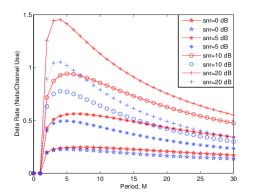
Figure 2: Achievable rates when $\alpha=0.90$ for SNR=0, 5,10, and 20 dB. The dotted lines provide rates when aliasing is taken into account, and the solid lines give the rates when aliasing is ignored.

In Figure 2, we plot the achievable rates when $\alpha=0.90$. Comparing Figs. 1 and 2, we observe that aliasing has a more significant impact as $\alpha$ decreases. This is expected since aliasing increases in a faster changing channel and hence ignoring aliasing provides a looser upper bound. When $\alpha=0.90$ and aliasing is taken into account, the optimal training periods are 7, 6, 5 and 4 for SNR values of 0, 5, 10 and 20 dB, respectively. When aliasing is ignored, the optimal values are 5, 5, 4 and 4, respectively. As before, the optimal period is decreasing and the effect of aliasing is increasing with the increasing SNR.

Figure 3 and Figure 4 are the bar graphs providing the optimal training and data power allocation for $\alpha=0.99$ and $0.90$, respectively, when the training period is at its optimal value. In the graphs, the first and the last bars give the power of the pilot symbols and the ones in between represent the data symbol power levels. These bar graphs are obtained when the effect of aliasing on the channel estimation is taken into account. We can immediately observe from both graphs that the data symbols farther away from the pilot symbols are allocated less power because the error in the estimation increases with the distance to the pilot symbols. In Fig. 3, the decrease in the allocated power is small since the channel is very slowly varying and estimate error is almost independent of $m$. On the other hand, the decrease is more obvious when the channel changes faster as evidenced in Fig. 4. Furthermore, comparing Figs. 3 and 4, we see that when the training period value is high, more power is allocated to the pilot symbol, enabling the system to track the channel more accurately.

VI-B Causal Filter Performance in the Absence of Aliasing

In this section, we study the performance when a causal Wiener filter is employed at the receiver. Since it is rather difficult to obtain the canonical factorization of arbitrary spectrums, we only consider cases in which the channel is slowly varying and the aliasing effect can be ignored. In Figure 5, we plot the achievable rates as a function of the training period for $\alpha=0.99$ when noncausal and causal Wiener filters are used. We compare the results when SNR$=0,5,10$ and $20$ dB. The dotted lines provide the rates for the case of the causal filter and the solid lines show the results for the case of the noncausal filter. We observe that the optimal training periods are 44, 29, 19 and 9 for the causal filter when SNR$=0,5,10$ and $20$, respectively. For the noncausal filter, the optimal periods are 25, 21, 16 and 8 for the same SNR values. We observe from the plots that the performance of causal and noncausal filters are very close. In Figure 6, we plot the achievable rates as a function of SNR at optimal periods obtained by using causal and noncausal filters. Again the performances are very similar. Moreover, after 45 dB, the rates are the same for both filters. Therefore, for the ranges of parameters considered in these figures, causal filter should be preferred over the noncausal one.

In systems where energy is at a premium, the energy required to send one bit of information is a metric that can be adopted to measure the efficiency of the system. The least amount of normalized bit energy required for reliable communications is given by $\frac{E_{b}}{N_{0}}=\frac{SNR}{C(SNR)}$ where $C(SNR)$ is the channel capacity in bits/symbol. In our setting, we use the achievable rates and analyze the required bit energy levels. In Figure 7, we plot the bit energy levels. The dashed and solid lines show the results for causal and noncausal filters. Note that the minimum bit energies are achieved at SNR = -4dB and -3dB for noncausal and causal filters, respectively. Operating below these SNR levels should be avoided as it only increases the required energy per bit. Figure 8 shows the optimal training period values as a function of SNR for both filters. Interestingly, the optimal period is increasing as SNR decreases for the causal filter while it first increases and then decreases when the noncausal filter is used. Since both past and future pilots are used when a noncausal filter is employed, having large training periods will diminish the benefits of future pilots especially for the data symbols in the middle. Therefore, this option is avoided in this case. On the other hand, having a larger period in the causal filter case enables the system to put more power to the pilot by not using data symbol slots farther away from the pilot and hence to obtain more accurate channel estimates. In both filters, as SNR increases the optimal period value stays constant at 5.

VII Conclusion

We have studied pilot-assisted communications when causal and noncausal Wiener filters are employed at the receiver for channel estimation. We have obtained achievable rate expressions by finding the error variances in both cases. Subsequently, we have jointly optimized the training period and power, and data power levels. We have analyzed the effects of aliasing on the data rates in Gauss-Markov Rayleigh fading channels when noncausal filters are used. We have provided numerical results showing the optimal parameters. We have compared the performances of causal and noncausal Wiener filters at different SNR values. We have also studied the energy-efficiency of pilot-assisted modulation with both filters.

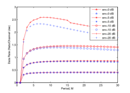
Figure 1: Achievable rates when $\alpha=0.99$ for SNR=0, 5,10, and 20 dB. The dotted lines provide rates when aliasing is taken into account, and the solid lines give the rates when aliasing is ignored.

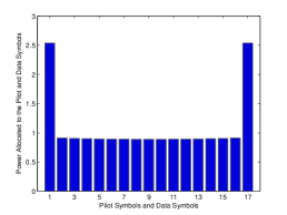
Figure 3: The optimal power distribution among the pilot and data symbols when $\alpha=0.99$ and SNR=0dB. The optimal period is 16.

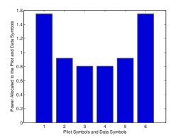
Figure 4: The optimal power distribution among the pilot and data symbols when $\alpha=0.90$ and SNR=0dB. The optimal period is 5.

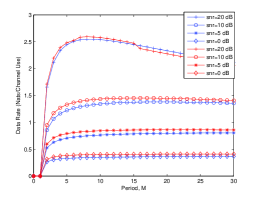
Figure 5: Achievable rates vs. training period when noncausal and causal filters are employed at the receiver. $\alpha=0.99$ and SNR=0, 5,10, and 20 dB. The solid lines give the rates when a noncausal filter is used and the dotted lines show the rates when a causal filter is used.

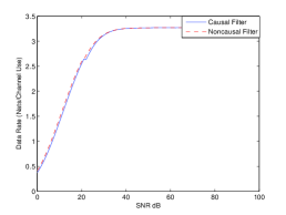
Figure 6: Achievable rates vs. SNR when noncausal and causal filters are employed at the receiver. $\alpha=0.99$. The dashed line gives the rate when a noncausal filter is used and the solid line shows the rate when a causal filter is used.

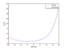
Figure 7: Bit energy $\frac{E_{b}}{N_{0}}$ vs. SNR(dB) when $\alpha=0.99$.

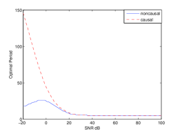
Figure 8: Optimal period vs. SNR(dB) for causal and noncausal filters when $\alpha=0.99$.

References

- [1] J.K. Cavers, “An analysis of pilot symbol assisted modulation for Rayleigh fading channels,” IEEE Trans. Vehicular Tech., vol. 40, pp. 686-693, November 1991.
- [2] J.K. Cavers, “Pilot assisted symbol modulation and differential detection in fading and delay spread,” IEEE Trans. Inform. Theory, vol. 43, no. 7, pp. 2206-2212, 1995.
- [3] S. Adireddy, L. Tong, and H. Viswanathan, “Optimal placement of training for unknown channels,” in Conference on Information Sciences and Systems, March 21-23, 2001.
- [4] B. Hassibi, and B. M. Hochwald, “How much training is needed in multiple-antenna wireless links?,” IEEE Trans. Inform. Theory, Vol. 49, pp.951-963, April 2003.
- [5] L. Tong, B.M. Sadler, and M. Dong, “Pilot-assisted wireless transmissions,” IEEE Signal Processing Magazine, vol. 21, no. 06, pp. 12-25, November 2004.
- [6] T. Kailath, A.H. Sayed, and B. Hassibi, “Linear Estimation,” Upper Saddle River, New Jersey: Prentice Hall, 2000.
- [7] S. Ohno and G.B. Giannakis, “Average-Rate Optimal PSAM Transmissions Over Time-Selective Fading Channels,” IEEE Trans. on Wireless Comm., Vol. 1, No. 4, October 2002.
- [8] J. Baltersee, G Fock, and H. Meyr, “An Information Theoretic Foundation of Synchronized Detection,” IEEE Trans. on Comm., Vol. 49, No. 12, December 2001.
- [9] J. Baltersee, G Fock, and H. Meyr, “Achievable Rate of MIMO Channels With Data-Aided Channel Estimation and Perfect Interleaving,” IEEE Journal on Selected Areas in Comm., Vol. 19, No. 12, December 2001.
- [10] I. Abou-Faycal, M. Mdard, and U. Madhow, “Binary adaptive coded pilot symbol assisted modulation over Rayleigh fading channels without feedback,” IEEE Trans. Commun., vol. 53, pp. 1036-1046, June 2005.
- [11] A. Bdeir, I. Abou-Faycal, and M. M edard , “Power allocation schemes for pilot symbol assisted modulation over rayleigh fading channels with no feedback,” Communications, IEEE International Conference on, vol. 2, pp. 737-741, June 2004.
- [12] M. F. Sencan, and M. C. Gursoy, “Achievable rates for pilot-assisted transmission over Rayleigh fading channels,” Proceedings of the 40th Annual Conference on Information Science and Systems, Princeton University, Princeton, NJ, March 22-24 2006.
- [13] S. Akin, and M. C. Gursoy, “Training Optimization for Gauss-Markov Rayleigh Fading Channels,” Proceedings of the 2007 IEEE International Conference on Communications, Glasgow, Scottland, UK, 24 28 June 2007.