To Cooperate, or Not to Cooperate in Imperfectly-Known Fading Channels

Abstract

In this paper, communication over imperfectly-known fading channels with different degrees of cooperation is studied. The three-node relay channel is considered. It is assumed that communication starts with the network training phase in which the receivers estimate the fading coefficients of their respective channels. In the data transmission phase, amplify-and-forward and decode-and-forward relaying schemes are employed. For different cooperation protocols, achievable rate expressions are obtained. These achievable rate expressions are then used to find the optimal resource allocation strategies. In particular, the fraction of total time or bandwidth that needs to be allocated to the relay for best performance is identified. Under a total power constraint, optimal allocation of power between the source and relay is investigated. Finally, bit energy requirements in the low-power regime are studied.

I Introduction

In wireless communications, deterioration in performance is experienced due to various impediments such as interference, fluctuations in power due to reflections and attenuation, and randomly-varying channel conditions caused by mobility and changing environment. Recently, cooperative wireless communications has attracted much interest as a technique that can mitigate these degradations and provide higher rates or improve the reliability through diversity gains. The relay channel was first introduced by van der Meulen in [1], and initial research is primarily conducted to understand the rates achieved in relay channels [2], [3]. More recently, diversity gains of cooperative transmission techniques have been studied in [4] and [5] where several two-user cooperative protocols have been proposed, with amplify-and-forward (AF) and decode-and-forward (DF) being the two basic modes. In [6], three different time-division AF and DF cooperative protocols with different the degrees of broadcasting and receive collision are studied. Most work in this area has assumed that the channel conditions are perfectly known at the receiver and/or transmitter sides. However, especially in mobile applications in which the channel changes randomly, the channel conditions can only be learned imperfectly.

In this paper, we study the impact of cooperation in imperfectly-known fading channels where a priori unknown fading coefficients are estimated at the receivers with the assistance of pilot symbols. We obtain achievable rates for AF and DF relaying techniques. Achievable rates are subsequently used to find the optimal fraction of total time or bandwidth allocated to the relay, enabling us to identify the optimal degree of cooperation. Under total power constraints, optimal power allocation strategies are determined. Moreover, we investigate the energy efficiency in the low-power regime.

II Channel Model

We consider the three-node relay network which consists of a source, destination, and a relay node. Source-destination, source-relay, and relay-destination channels are modeled as Rayleigh block-fading channels with fading coefficients denoted by $h_{sr}$, $h_{sd}$, and $h_{rd}$, respectively for each channel. Due to the block-fading assumption, the fading coefficients $h_{sr}\sim\mathcal{C}\mathcal{N}(0,{\sigma_{sr}}^{2})$, $h_{sd}\sim\mathcal{C}\mathcal{N}(0,{\sigma_{sd}}^{2})$, and $h_{rd}\sim\mathcal{C}\mathcal{N}(0,{\sigma_{rd}}^{2})$ stay constant for a block of $m$ symbols before they assume independent realizations for the following block. It is assumed that the source, relay, and destination nodes do not have prior knowledge of the instantaneous realizations of the fading coefficients. Hence, the transmission is conducted in two phases: network training phase in which the fading coefficients are estimated at the receivers, and data transmission phase. Overall, the source and relay are subject to the following power constraints in one block: $\|{\mathbf{x}_{s,t}}\|^{2}+E\{\|{\mathbf{x}_{s}}\|^{2}\}\leq mP_{s}$ and $\|{\mathbf{x}_{r,t}}\|^{2}+E\{\|{\mathbf{x}_{r}}\|^{2}\}\leq mP_{r}$ where $\mathbf{x}_{s,t}$ and $\mathbf{x}_{r,t}$ are the source and relay training signal vectors, respectively, and $\mathbf{x}_{s}$ and $\mathbf{x}_{r}$ are the corresponding source and relay data vectors.

II-A Network Training Phase

Each block transmission starts with the training phase. In the first symbol period, source transmits a pilot symbol to enable the relay and destination to estimate channel coefficients $h_{sr}$ and $h_{sd}$. In the average power limited case, sending a single pilot is optimal because instead of increasing the number of pilot symbols, a single pilot with higher power can be used. The signals received by the relay and destination, respectively, are $y_{r,t}=h_{sr}x_{s,t}+n_{r}$ and $y_{d,t}=h_{sd}x_{s,t}+n_{d}$. Similarly, in the second symbol period, relay transmits a pilot symbol to enable the destination to estimate the channel coefficient $h_{rd}$. The signal received by the destination is $y_{d,t}^{r}=h_{rd}x_{r,t}+n_{d}^{r}$. In the above formulations, $n_{r}\sim\mathcal{C}\mathcal{N}(0,N_{0})$, $n_{d}\sim\mathcal{C}\mathcal{N}(0,N_{0})$, and $n_{d}^{r}\sim\mathcal{C}\mathcal{N}(0,N_{0})$ represent independent Gaussian noise samples at the relay and the destination nodes.

In the training process, it is assumed that the receivers employ minimum mean-square error (MMSE) estimation. Let us assume that the source allocates $\delta_{s}$ of its total power for training while the relay allocates $\delta_{r}$ of its total power for training. As described in [8], the MMSE estimate of $h_{sr}$ is given by $\hat{h}_{sr}=\frac{\sigma_{sr}^{2}\sqrt{\delta_{s}mP_{s}}}{\sigma_{sr}^{2}\delta_{s}mP_{s}+N_{0}}y_{r,t}$ where $y_{r,t}\sim\mathcal{C}\mathcal{N}(0,\sigma_{sr}^{2}\delta_{s}mP_{s}+N_{0})$. We denoted by $\tilde{h}_{sr}$ the estimate error which is a zero-mean complex Gaussian random variable with variance $var(\tilde{h}_{sr})=\frac{\sigma_{sr}^{2}N_{0}}{\sigma_{sr}^{2}\delta_{s}mP_{s}+N_{0}}$. Note that we can write $h_{sr}=\hat{h}_{sr}+\tilde{h}_{sr}$. Similar expressions are obtained for $\hat{h}_{sd},\tilde{h}_{sd},\hat{h}_{rd}$, and $\tilde{h}_{rd}$ which are the estimates and estimate errors of the fading coefficients $h_{sd}$ and $h_{rd}$, respectively.

II-B Data Transmission Phase

The practical relay node usually cannot transmit and receive data simultaneously. Thus, we assume that the relay works under half-duplex constraint. As discussed in the previous section, within a block of $m$ symbols, the first two symbols are allocated for channel training. In the remaining duration of $m-2$ symbols, data transmission takes place. We introduce the relay transmission parameter $\alpha$ and assume that $\alpha(m-2)$ symbols are allocated for relay transmission. Hence, $\alpha$ can be seen as the fraction of total time or bandwidth allocated to the relay. Note that the parameter $\alpha$ enables us to control the degree of cooperation. In this paper, we consider three relaying schemes: Amplify and Forward, Decode and Forward with repetition channel coding, and Decode and Forward with parallel channel coding.

II-B1 AF and repetition DF

In AF and repetition DF, since the relay either amplifies the received signal, or decodes it but uses the same codebook as the source to forward the data, cooperative transmission takes place in the duration of $2\alpha(m-2)$ symbols. The remaining duration of $(1-2\alpha)(m-2)$ symbols is allocated to unaided direct transmission from the source to the destination. It is obvious that we have $0<\alpha\leq 1/2$ in this setting. Therefore, $\alpha=1/2$ models full cooperation while we have noncooperative communications as $\alpha\to 0$.

In these protocols, the input-output relations are expressed as follows: $\mathbf{y}_{d1}=h_{sd}\mathbf{x}_{s1}+\mathbf{n}_{d}$, $\mathbf{y}_{r}=h_{sr}\mathbf{x}_{s21}+\mathbf{n}_{r}$, $\mathbf{y}_{d2}=h_{sd}\mathbf{x}_{s21}+\mathbf{n}_{d}$, $\mathbf{y}_{d}^{r}=h_{sd}\mathbf{x}_{s22}+h_{rd}\mathbf{x}_{r}+\mathbf{n}_{d}^{r}$. Above, $\mathbf{x}_{s1},\mathbf{x}_{s21},\mathbf{x}_{s22}$, which have respective dimensions $(1-2\alpha)(m-2)$, $\alpha(m-2)$ and $\alpha(m-2)$, represent the source data vectors sent in direct transmission, cooperative transmission when relay is listening and cooperative transmission when relay is transmitting, respectively. Note that we assume in this case that the source transmits all the time. $\mathbf{x}_{r}$ is the relay’s data vector with dimension $\alpha(m-2)$. $\mathbf{y}_{d1},\mathbf{y}_{d2},\mathbf{y}_{d}^{r}$ are the corresponding received vectors at the destination, and $\mathbf{y}_{r}$ is the received vector at the relay. The input vector $\mathbf{x}_{s}$ now is defined as $\mathbf{x}_{s}=[\mathbf{x}_{s1}^{T},\mathbf{x}_{s21}^{T},\mathbf{x}_{s22}^{T}]^{T}$, and $\mathbf{x}_{s}$ and $\mathbf{x}_{r}$ vectors are assumed to be composed of independent random variables with equal energy. Hence, the corresponding covariance matrices are

$$E\{\mathbf{x}_{s}\mathbf{x}_{s}^{\dagger}\}=P_{s}^{\prime}\,\,\mathbf{I}=\frac{(1-\delta_{s})mP_{s}}{m-2}\,\,\mathbf{I},$$ (1)

$$E\{\mathbf{x}_{r}\mathbf{x}_{r}^{\dagger}\}=P_{r}^{\prime}\,\,\mathbf{I}=\frac{(1-\delta_{r})mP_{r}}{(m-2)\alpha}\,\,\mathbf{I}.$$ (2)

II-B2 Parallel DF

In DF with parallel channel coding, we simplify the transmission by assuming that the source becomes silent while relay is transmitting information. Thus, source transmits over a duration of $(1-\alpha)(m-2)$ symbols. Now, the range of $\alpha$ is $0<\alpha<1$. In this case, the input-output relations are given by: $\mathbf{y}_{r}=h_{sr}\mathbf{x}_{s}+\mathbf{n}_{r}$, $\mathbf{y}_{d}=h_{sd}\mathbf{x}_{s}+\mathbf{n}_{d}$, $\mathbf{y}_{d}^{r}=h_{rd}\mathbf{x}_{r}+\mathbf{n}_{d}^{r}$. The dimensions of the vectors $\mathbf{x}_{s},\mathbf{y}_{d},\mathbf{y}_{r}$ are $(1-\alpha)(m-2)$, while $\mathbf{x}_{r},\mathbf{y}_{d}^{r}$ are vectors of dimension $\alpha(m-2)$. In this case, the covariance matrix for relay data vector remains the same in as (2) while the covariance for source data vector $\mathbf{x}_{s}$ is

$$E\{\mathbf{x}_{s}\mathbf{x}_{s}^{\dagger}\}=P_{s1}^{\prime}\,\,\mathbf{I}=\frac{(1-\delta_{s})mP_{s}}{(m-2)(1-\alpha)}\,\,\mathbf{I}.$$ (3)

III Achievable Rates

In this section, we find achievable rate expressions for the three relaying protocols described in Section II. Using the same techniques described in [7], we can show that capacity lower bounds are obtained when the channel estimation error is assumed to be another source of Gaussian noise. This is due to the fact that Gaussian noise is the worst uncorrelated noise for the Gaussian model. The achievable rate expressions are provided below. The proofs are omitted due to lack of space.

Theorem 1

An achievable rate expression for AF transmission scheme is given by

$$I_{low}= \frac{1}{m}E\Bigg{\{}\Bigg{[}(1-2\alpha)(m-2)\log(1+\frac{P_{s}^{\prime}|\hat{h}_{sd}|^{2}}{\sigma_{z_{d}}^{2}})+(m-2)\alpha$$

$$\log\Big{(}1+\frac{P_{s}^{\prime}|\hat{h}_{sd}|^{2}}{\sigma_{z_{d}}^{2}}+f\bigg{(}\frac{P_{s}^{\prime}|\hat{h}_{sr}|^{2}}{\sigma_{z_{r}}^{2}},\frac{P_{r}^{\prime}|\hat{h}_{rd}|^{2}}{\sigma_{z_{d}^{r}}^{2}}\bigg{)}$$

$$+q\bigg{(}\frac{P_{s}^{\prime}|\hat{h}_{sd}|^{2}}{\sigma_{z_{d}}^{2}},\frac{P_{s}^{\prime}|\hat{h}_{sd}|^{2}}{\sigma_{z_{d}^{r}}^{2}},\frac{P_{s}^{\prime}|\hat{h}_{sr}|^{2}}{\sigma_{z_{r}}^{2}},\frac{P_{r}^{\prime}|\hat{h}_{rd}|^{2}}{\sigma_{z_{d}^{r}}^{2}}\bigg{)}\Big{)}\Bigg{]}\Bigg{\}}$$ (4)

where $f(.)$, $q(.)$ are defined as $f(x,y)=\frac{xy}{1+x+y}$ ,$q(a,b,c,d)=\frac{(1+a)b(1+c)}{1+c+d}$. Moreover

$$\frac{P_{s}^{\prime}|\hat{h}_{sd}|^{2}}{\sigma_{z_{d}}^{2}}=\frac{\delta_{s}(1-\delta_{s})m^{2}P_{s}^{2}\sigma_{sd}^{4}}{(1-\delta_{s})mP_{s}\sigma_{sd}^{2}N_{0}+(m-2)(\sigma_{sd}^{2}\delta_{s}mP_{s}+N_{0})N_{0}}|w_{sd}|^{2}$$ (5)

$$\frac{P_{s}^{\prime}|\hat{h}_{sr}|^{2}}{\sigma_{z_{r}}^{2}}=\frac{\delta_{s}(1-\delta_{s})m^{2}P_{s}^{2}\sigma_{sr}^{4}}{(1-\delta_{s})mP_{s}\sigma_{sr}^{2}N_{0}+(m-2)(\sigma_{sr}^{2}\delta_{s}mP_{s}+N_{0})N_{0}}|w_{sr}|^{2}$$ (6)

$$\frac{P_{s}^{\prime}|\hat{h}_{sd}|^{2}}{\sigma_{z_{d}^{r}}^{2}}=\frac{\delta_{s}(1-\delta_{s})m^{2}P_{s}^{2}\sigma_{sd}^{4}(\sigma_{rd}^{2}\delta_{r}mP_{r}+N_{0})}{(m-2)(\sigma_{sd}^{2}\delta_{s}mP_{s}+N_{0})(\sigma_{rd}^{2}\delta_{r}mP_{r}+N_{0})N_{0}}$$

$$\frac{}{+(1-\delta_{r})mP_{r}\sigma_{rd}^{2}N_{0}(\sigma_{sd}^{2}\delta_{s}mP_{s}+N_{0})/\alpha}$$

$$\frac{}{+(1-\delta_{s})mP_{s}\sigma_{sd}^{2}N_{0}(\sigma_{rd}^{2}\delta_{r}mP_{r}+N_{0})}|w_{sd}|^{2}$$ (7)

$$\frac{P_{r}^{\prime}|\hat{h}_{rd}|^{2}}{\sigma_{z_{d}^{r}}^{2}}=\frac{\delta_{r}(1-\delta_{r})m^{2}P_{r}^{2}\sigma_{rd}^{4}(\sigma_{sd}^{2}\delta_{s}mP_{s}+N_{0})/\alpha}{(m-2)(\sigma_{sd}^{2}\delta_{s}mP_{s}+N_{0})(\sigma_{rd}^{2}\delta_{r}mP_{r}+N_{0})N_{0}}$$

$$\frac{}{+(1-\delta_{r})mP_{r}\sigma_{rd}^{2}N_{0}(\sigma_{sd}^{2}\delta_{s}mP_{s}+N_{0})/\alpha}$$

$$\frac{}{+(1-\delta_{s})mP_{s}\sigma_{sd}^{2}N_{0}(\sigma_{rd}^{2}\delta_{r}mP_{r}+N_{0})}|w_{rd}|^{2}$$ (8)

and here and henceforth $w_{sr},w_{sd},w_{rd}$ are i.i.d with distribution $\mathcal{C}\mathcal{N}(0,1)$.

Theorem 2

An achievable rate expression for DF with repetition channel coding transmission scheme is given by

$$I_{low}=\frac{1}{m}\Big{\{}(1-2\alpha)(m-2)E_{w_{sd}}\log(1+\frac{P_{s}^{\prime}|\hat{h}_{sd}|^{2}}{\sigma_{z_{d}}^{2}})+(m-2)\alpha\min\{I_{1},I_{2}\}\Big{\}}$$ (9)

where

$$I_{1}=E_{w_{sr}}\Bigg{[}\log\Bigg{(}1+\frac{P_{s}^{\prime}|\hat{h}_{sr}|^{2}}{\sigma_{z_{r}}^{2}}\Bigg{)}\Bigg{]},$$ (10)

$$I_{2}=E_{w_{sd}}E_{w_{rd}}\Bigg{[}\log\Big{(}1+\frac{P_{s}^{\prime}|\hat{h}_{sd}|^{2}}{\sigma_{z_{d}}^{2}}+\frac{P_{r}^{\prime}|\hat{h}_{rd}|^{2}}{\sigma_{z_{d}^{r}}^{2}}$$

$$+\frac{P_{s}^{\prime}|\hat{h}_{sd}|^{2}}{\sigma_{z_{d}^{r}}^{2}}+\frac{P_{s}^{\prime}|\hat{h}_{sd}|^{2}}{\sigma_{z_{d}}^{2}}\frac{P_{s}^{\prime}|\hat{h}_{sd}|^{2}}{\sigma_{z_{d}^{r}}^{2}}\Big{)}\Bigg{]}$$ (11)

where $\frac{P_{s}^{\prime}|\hat{h}_{sd}|^{2}}{\sigma_{z_{d}}^{2}}$, $\frac{P_{s}^{\prime}|\hat{h}_{sr}|^{2}}{\sigma_{z_{r}}^{2}}$,$\frac{P_{s}^{\prime}|\hat{h}_{sd}|^{2}}{\sigma_{z_{d}^{r}}^{2}}$, $\frac{P_{r}^{\prime}|\hat{h}_{rd}|^{2}}{\sigma_{z_{d}^{r}}^{2}}$ are the same as in (5)-(1)

With regard to parallel DF, based on [9], we can write the capacity lower bound as

$$I_{low}=\sup_{p_{x_{s}}(\cdot),p_{x_{r}}(\cdot)}\min\{ (1-\alpha)\emph{I}(\mathbf{x}_{s};\mathbf{y}_{r}|\hat{h}_{sr}),(1-\alpha)\emph{I}(\mathbf{x}_{s};\mathbf{y}_{d}|\hat{h}_{sd})$$

$$+\alpha\emph{I}(\mathbf{x}_{r};\mathbf{y}_{d}^{r}|\hat{h}_{rd})\}.$$

Using similar methods as before, we obtain the following result.

Theorem 3

An achievable rate of DF with parallel channel coding scheme is given by

$$I_{low}=\min\Bigg{\{}E\left\{\frac{(1-\alpha)(m-2)}{m}\log\Big{(}1+\frac{P_{s1}^{\prime}|\hat{h}_{sr}|^{2}}{\sigma_{z_{r1}}^{2}}\Big{)}\right\},$$

$$E\left\{\frac{(1-\alpha)(m-2)}{m}\log\Big{(}1+\frac{P_{s1}^{\prime}|\hat{h}_{sd}|^{2}}{\sigma_{z_{d1}}^{2}}\Big{)}\right.+$$

$$\left.\frac{\alpha(m-2)}{m}\log\Big{(}1+\frac{P_{r1}^{\prime}|\hat{h}_{rd}|^{2}}{\sigma_{z_{d1}^{r}}^{2}}\Big{)}\Bigg{\}}\right\}$$

where

$$\frac{P_{s1}^{\prime}|\hat{h}_{sd}|^{2}}{\sigma_{z_{d1}}^{2}}=\frac{\delta_{s}(1-\delta_{s})m^{2}P_{s}^{2}\sigma_{sd}^{4}/(1-\alpha)|w_{sd}|^{2}}{(1-\delta_{s})mP_{s}\sigma_{sd}^{2}N_{0}/(1-\alpha)+(m-2)(\sigma_{sd}^{2}\delta_{s}mP_{s}+N_{0})N_{0}}$$

$$\frac{P_{s1}^{\prime}|\hat{h}_{sr}|^{2}}{\sigma_{z_{r1}}^{2}}=\frac{\delta_{s}(1-\delta_{s})m^{2}P_{s}^{2}\sigma_{sr}^{4}/(1-\alpha)|w_{sr}|^{2}}{(1-\delta_{s})mP_{s}\sigma_{sr}^{2}N_{0}/(1-\alpha)+(m-2)(\sigma_{sr}^{2}\delta_{s}mP_{s}+N_{0})N_{0}}$$

$$\frac{P_{r1}^{\prime}|\hat{h}_{rd}|^{2}}{\sigma_{z_{d1}^{r}}^{2}}=\frac{\delta_{r}(1-\delta_{r})m^{2}P_{r}^{2}\sigma_{rd}^{4}/\alpha|w_{rd}|^{2}}{(1-\delta_{r})mP_{r}\sigma_{rd}^{2}N_{0}/\alpha+(m-2)(\sigma_{rd}^{2}\delta_{s}mP_{r}+N_{0})N_{0}}$$

IV Numerical Results

We first analyze the effect of the degree of cooperation on the performance in AF and repetition DF. Figures 1-4 plot the achievable rates as a function of $\alpha$. Achievable rates are obtained for different channel qualities given by the standard deviations $\sigma_{sd},\sigma_{sr},$ and $\sigma_{rd}$ of the fading coefficients.

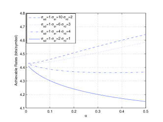
Figure 1: AF achievable rate vs. $\alpha$ when $P_{s}=P_{r}=50,\delta_{s}=\delta_{r}=0.1$

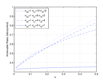
Figure 2: AF achievable rate vs. $\alpha$ when $P_{s}=P_{r}=0.5,\delta_{s}=\delta_{r}=0.1$

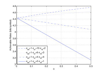
Figure 3: DF with repetition coding achievable rate vs. $\alpha$ when $P_{s}=P_{r}=50,\delta_{s}=\delta_{r}=0.1$

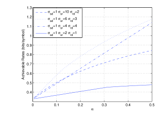
Figure 4: DF with repetition coding achievable rate vs. $\alpha$ when $P_{s}=P_{r}=0.5,\delta_{s}=\delta_{r}=0.1$

We observe that if the input power is high, $\alpha$ should be either $0.5$ or close to zero depending on the channel qualities. On the other hand, $\alpha=0.5$ always gives us the best performance at low SNR levels regardless of the channel qualities. Hence, while cooperation is beneficial in the low-SNR regime, noncooperative transmissions might be optimal at high SNRs. We note from Fig. 1 that cooperation starts being useful as the source-relay channel variance $\sigma^{2}_{sr}$ increases. Similar results are also observed in Fig 3. Hence, the source-relay channel quality is one of the key factors in determining the usefulness of cooperation in the high SNR regime.

We now consider the special case of $\alpha=0.5$ which provides the maximum of degree of cooperation. In certain cases, source and relay are subject to a total power constraint. Here, we introduce the power allocation coefficient $\theta$, and total power constraint $P$. $P_{s}$ and $P_{r}$ have the following relations: $P_{s}=\theta P$, $P_{r}=(1-\theta)P$, and $P_{s}+P_{r}\leq P$. Next, we investigate how different values of $\theta$, and hence different power allocation strategies, affect the achievable rates. Figures 5-7 plot the achievable rates as a function of $\theta$ for AF and DF. In the figures, we have assumed that $N_{0}=1,\delta_{s}=0.1,\delta_{r}=0.1$. Note that the rates for $\theta=1$ do not exactly correspond to the rates of direct transmission in which no time is used for training for relay channels. Therefore, for fair comparison, we also provide the direct transmission rates in the figures.

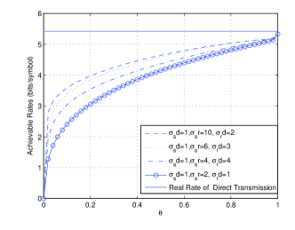
Figure 5: AF achievable rate vs. $\theta$. $P=100$.

In Fig. 5 where $P=100$, we observe that direct transmission without the relay is superior in this high SNR case. On the other hand, we see different results when we turn our attention to the low-SNR regime. Figs. 6 and 7 provide the achievable rates of AF and DF, respectively, when $P=1$. We observe in these cases that relaying increases the rates and hence cooperation is useful unless the source-relay and relay-destination channel qualities are comparable to that of the source-destination channel.

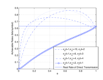
Figure 6: AF achievable rate vs. $\theta$. $P=1$.

.

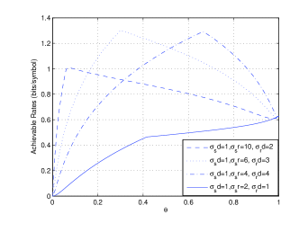
Figure 7: DF with repetition coding rate vs. $\theta$. $P=1$. Direct transmission rate is the same as in Fig. 6.

Finally, in Fig. 8, we plot the achievable rates of DF parallel channel coding, derived in Theorem 3. We can see from the figure that the best performance is obtained when the source-relay channel quality is high (i.e., when $\sigma_{sd}=1,\sigma_{sr}=10,\sigma_{rd}=2$). Additionally, we observe that as the source-relay channel improves, more resources need to be allocated to the relay to achieve the best performance. We note that significant improvements with respect to direct transmission (i.e., $\alpha\to 0$) are obtained. Finally, we can see that when compared to AF and DF with repetition coding, DF with parallel channel coding achieves higher rates. On the other hand, AF and DF with repetition coding have implementation advantages.

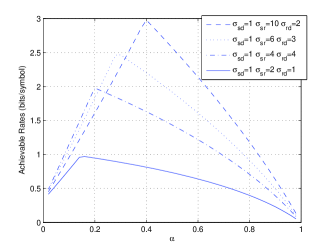
Figure 8: DF parallel coding achievable rate vs. $\alpha$ when $P_{s}=P_{r}=0.5,\delta_{s}=\delta_{r}=0.1$

V energy efficiency

Our analysis has shown that cooperative relaying is generally beneficial in the low-power regime, resulting in improved achievable rates when compared to direct transmission. In this section, we provide an energy efficiency perspective. The least amount of energy required to send one information bit reliably is given by $\frac{E_{b}}{N_{0}}=\frac{{\text{\footnotesize{SNR}}}}{C({\text{\footnotesize{SNR}}})}$ where $C({\text{\footnotesize{SNR}}})$ is the channel capacity in bits/symbol. In our setting, the bit energy values are given by $\frac{E_{b,U}}{N_{0}}=\frac{{\text{\footnotesize{SNR}}}}{I_{low}({\text{\footnotesize{SNR}}})}$. $\frac{E_{b,U}}{N_{0}}$ provides the least amount of normalized bit energy values in the worst-case scenario and also serves as an upper bound on the achievable bit energy levels of the channel. We note that we define the signal-to-noise ratio as ${\text{\footnotesize{SNR}}}=P/N_{0}$ where $P$ is the total power in the system. The next result provides the asymptotic behavior of the bit energy as SNR decreases to zero.

Theorem 4

The normalized bit energy in all transmission schemes grows without bound as the signal-to-noise ratio decreases to zero, i.e.,

$$\left.\frac{E_{b,U}}{N_{0}}\right|_{I_{low}=0}=\lim_{{\text{\footnotesize{SNR}}}\to 0}\frac{{\text{\footnotesize{SNR}}}}{I_{low}({\text{\footnotesize{SNR}}})}=\frac{1}{\dot{I}_{low}(0)}=\infty.$$ (12)

The result is shown easily by proving in all relaying protocols that $\dot{I}_{low}(0)=0$. Theorem 4 indicates that it is extremely energy-inefficient to operate at very low SNR values. In general, it is not easy to identify the most energy-efficient operating points analytically. Therefore, we resort to numerical analysis. We choose the following numerical values for the following parameters: $\delta_{s}=\delta_{r}=0.1$, $\sigma_{sd}=1$, $\sigma_{sr}=4$, $\sigma_{rd}=4$, $\alpha=0.5$, and $\theta=0.6$. Fig. 9 plots the bit energy curves as a function of SNR for different values of $m$ in the AF case. We can see from the figure that the minimum bit energy, which is achieved at a nonzero value of SNR, decreases with increasing $m$ and is achieved at a lower SNR value. Fig. 10 shows the minimum bit energy for different relaying schemes with overlapped or non-overlapped transmission techniques. In non-overlapped transmission, source becomes silent while the relay transmits. The achievable rates of non-overlapped DF with parallel coding are provided in Theorem 3. The non-overlapped AF and DF with repetition coding are considered in [7]. In overlapped transmission, source continues its transmission as the relay transmits. The rates for overlapped AF and DF with repetition coding are given in Theorems 1 and 2. We observe in Fig. 10 that the minimum bit energy decreases with increasing $m$ in all cases . We realize that DF is in general much more energy-efficient than AF. Moreover, we note that surprisingly employing non-overlapped rather than overlapped transmission improves the energy efficiency.

Figure 9: AF $E_{b,U}/N_{0}$ vs. SNR

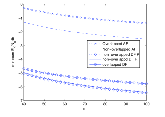
Figure 10: $E_{b,U}/N_{0}$ vs. $m$ for different transmission scheme. P denotes parallel channel coding while R denotes repetition channel coding.

References

• [1] E. C. van der Meulen, Three-terminal communication channels, Adv. Appl. Probab., vol. 3, pp. 120 C154, 1971.
• [2] T. M. Cover and A.A. El Gamal, Capacity theorems for the relay channel, IEEE Trans. Inf. Theory, vol. IT-25, no. 5, pp. 572 C584, Sep. 1979.
• [3] A. A. El Gamal and M. Aref, The capacity of the semideterministic relay channel, IEEE Trans. Inf. Theory, vol. IT-28, no. 3, pp. 536 C536, May 1982.
• [4] J.N. Laneman, D.N.C. Tse, G.W. Wornel “Cooperative diversity in wireless networks: Efficient protocols and outage behavior,” IEEE Trans. Inform. Theory, vol.50,pp.3062-3080. Dec.2004
• [5] J. N. Laneman, “Cooperation in wireless networks: Principles and applications,” Springer, 2006, ch.1 Cooperative Diversity: Models, Algorithms, and Architectures
• [6] R.U. Nabar, H. Bolcskei, F.W. Kneubuhler, “Fading Relay Channels:Performance Limits and Space-Time Signal Design,” IEEE J.Select. Areas Commun vol.22,NO.6 pp1099-1109. Aug.2004
• [7] J.Zhang, M.C.Gursoy, “Achievable Rates and Optimal Resource Allocation for Imperfectly-Known Relay Channels,” 45th Annual Allerton Conference on Communication, Control, and Computing,UIUC Sep. 2007.
• [8] M.C. Gursoy, “An energy efficiency perspective on training for fading channels,” Proceedings of the IEEE ISIT 2007.
• [9] Yingbin Liang, Venugopal V. Veeravalli,“Gaussian Orthogonal Relay Channels: Optimal Resource Allocation and Capacity,”IEEE Trans. Inform. Theory, vol.51,pp.3284- 3289. Sep.2005