Bayesian estimation of one-parameter qubit gates

Abstract

We address estimation of one-parameter unitary gates for qubit systems and seek for optimal probes and measurements. Single- and two-qubit probes are analyzed in details focusing on precision and stability of the estimation procedure. Bayesian inference is employed and compared with the ultimate quantum limits to precision, taking into account the biased nature of Bayes estimator in the non asymptotic regime. Besides, through the evaluation of the asymptotic a posteriori distribution for the gate parameter and the comparison with the results of Monte Carlo simulated experiments, we show that asymptotic optimality of Bayes estimator is actually achieved after a limited number of runs. The robustness of the estimation procedure against fluctuations of the measurement settings is investigated and the use of entanglement to improve the overall stability of the estimation scheme is also analyzed in some details.

1 Introduction

Let us consider a system prepared in a known quantum state which enters an apparatus performing an operation on the state. The evolution imposed by the apparatus depends on the value of some parameters and the experimenter is interested in the estimation of those parameters. A natural strategy to obtain the parameter is to detect the state at the output and infer the value of the parameters from the global sample coming from a number of repeated measurements. The optimization of this strategy, i.e. the choice of the best probe, measurement and data processing, is the subject of quantum parameter estimation, which is a relevant subject in the quantum characterization of states and operations [1, 2]. The operation on the state may be unitary or not [3, 4] and may depend on one or more unknown parameters, which, in turn, may correspond to quantities that are not directly observable. The parameters of interest may be the amplitude of the carrier signal, the position and orientation of an object, or the strength of an external fields. Communications, image analysis and precision metrology provide relevant examples. In the simplest scenario, a parameter estimation problem consists in the determination of the value of the interaction parameter $\theta$ for unitaries of the form $U_{\theta}=\{-i\theta G\}$ where $G$ is a Hamiltonian operator that generates the transformation.

Generally speaking, quantum estimation is concerned with the problem of finding optimal ways to estimate quantum states and processes. In turn, it has recently attracted much interest in quantum information [5, 6, 7, 8, 9] as a tool for characterization of signal and gates at the quantum level [10, 11, 12, 13, 14, 15, 16, 17, 18]. The canonical way to address estimation of states and operation is by quantum tomography, (see [19] for a review) i.e by measuring a complete set (a quorom [14]) of observables, which allows or the complete characterization. For single- and two-qubit systems this involves the measurement of Pauli matrices and has been realized for polarization qubits [20, 21]. Process Tomography, i.e the reconstruction of quantum operations [22, 23, 24], is itself critical for verifying the actions of quantum logic gates [25] and characterizing decoherence processes [26]. On the other hand, there are many situations where the full tomography of signals and devices is not needed, either because the focus is on specific features of the transformation, or the dynamics is partially known. In this cases the relevant point is to find an optimal and stable way to achieve quantum characterization by parameter estimation. For this reason, in this paper we address estimation of one-parameter unitary gates for qubit systems, i.e. transformation of the form $U_{\theta}=\{-i\theta G\}$ where $G$ is a combination of Pauli operators and $\theta$ is the parameter of interest. We consider the gate probed either by one-qubit and two-qubit states and compare the performances of standard measurements with the ultimate quantum limit to precision (accuracy) of estimation. As we will see, ultimate bounds are determined by the initial quantum state of the probe, the type of interaction and the readout measurements that is used to extract information from the probe. In particular, we are going to assess the performances of Bayes estimators, which themselves play a central role in many signal processing problems [27].

The precision (variance) of any unbiased estimator of a parameter $\theta$ is limited by the Cramér-Rao bound (CR), given by the inverse of the Fisher information [7, 28, 29, 30, 31, 32, 33]. Bayes estimators are known to be asymptotically unbiased and, in turn, to saturate CR asymptotically. For measurements that are related to the unknown $\theta$ through a linear Gaussian model, the maximum likelihood estimate of $\theta$ also achieves the CR. Furthermore, when $\theta$ is estimated from independent identically distributed (iid) measurements, under suitable regularity assumptions on the probability density, the maximum likelihood estimator is asymptotically unbiased and achieves the CR [29, 34]. On the other hand, being interested in realistic measurement schemes, here we consider estimation procedure based on a limited number of measurements. As a consequence, we have to take into account the biased nature of Bayes estimators. The variance of any estimator with a given bias is bounded by the biased CR [35, 36], which is an extension of the CR taking into account the a priori distribution of the parameter of interest. In turn, it is a fundamental rule of estimation theory that the use of prior knowledge leads to a more accurate estimator.

In this paper we address the estimation of the interaction parameter of unitary qubit transformations. We derive ultimate quantum limits to precision and assess performances of Bayesian estimators [37, 38]. In particular, we focus our attention on measurement schemes as those in Fig. 1 and Fig. 5, where a single-qubit gate is probed by single- and two-qubit probes, respectively. We evaluate the a posteriori distribution for the gate parameter, derive the ultimate bound on precision, and compare the asymptotic performances of Bayes estimator to that of Monte Carlo simulated experiments, thus showing that asymptotic optimality is achieved after a limited number of runs. The paper is structured as follows. In Section 2 we introduce notation and derive the a posteriori distribution, also discussing the Bayesian version of the CRB. In Section 3 we discuss limits to precision in estimating unitary gates for qubit systems. A comparison between single- and two-qubit entangled probes shows that entanglement improves the overall stability of the estimation procedure. We also compare the asymptotic a posteriori distribution for the gate parameter to the results of the Monte Carlo simulated experiments. Section 4 closes the paper with some concluding remarks.

2 Parameter estimation of one-parameter qubit gates

A generic unitary transformation acting on a qubit state can be written as $U({\boldsymbol{\theta}})=\exp\{-\frac{i}{2}{\boldsymbol{\theta}}\cdot{\boldsymbol{\sigma}}\}$, where ${\boldsymbol{\sigma}}=\{\boldsymbol{\sigma}_{1},\boldsymbol{\sigma}_{2},\boldsymbol{\sigma}_{3}\}$ is the vector of Pauli matrices and ${\boldsymbol{\theta}}$ is a vector describing the transformation. In the following we will assume that ${\boldsymbol{\theta}}$ depends on a single parameter and refer to it as to $\theta$. The simplest scheme for the estimation of $\theta$ [1] consists in choosing a probe pure qubit state $|\psi_{0}\rangle$ undergoing the transformation and a measurement onto the evolved state $|\psi_{\theta}\rangle\equiv U({\theta})|\psi_{0}\rangle$. Here we assume that the measurement can be represented by the two projectors $\Pi_{0}$ and $\Pi_{1}$, so that the conditional probabilities to obtain the outcomes “0” or “1” (i.e. given $\theta$) are $P(j|\theta)=\langle\psi_{\theta}|\Pi_{j}|\psi_{\theta}\rangle$, $j=0,1$. After $M$ measurements on equally prepared qubits we have the the sample $X=\{x_{1},\ldots,x_{M}\}$ of outcomes, where the $x_{k}$’s can take the values “0” and “1”. This leads us to define the following sample probability or likelihood function:

$$P(X|\theta)=\prod_{k=1}^{M}P(x_{k}|\theta).$$ (1)

Our estimation problem is that of inferring the value of $\theta$ once the sample of outcomes is assigned by the measurement; in other words, we are interested in the conditional (a posteriori) probability $P(\theta|X)$ of $\theta$ given the sample $X$. This can be easily obtained by the Bayes theorem, which states that [39, 40] $P(\theta|X)P(\theta)=P(X|\theta)P(X)$ where $P(\theta)$ is the prior probability and $P(X)$ is the overall (unconditional) probability of the observed sample. Hence, the a posteriori distribution may be written as

$$P(\theta|X)=\frac{1}{N}\prod_{k=1}^{M}P(x_{k}|\theta)\,,\qquad{N}=\int_{\Omega}\!\!\!d\theta\prod_{k=1}^{M}P(x_{k}|\theta)\,,$$ (2)

where ${N}$ is the normalization and $\Omega$ is the set of possible values for $\theta$. From (2) we may evaluate the expected value of $\theta$ and the variance of the distribution

$$\overline{\theta}=\int_{\Omega}\!\!\!d\theta\,\theta\,P(\theta|X),\quad\quad{\rm Var}[\theta]=\int_{\Omega}\!\!\!d\theta\,(\theta-\overline{\theta})^{2}\,P(\theta|X)\>.$$ (3)

The mean (expected) value $\overline{\theta}$ of the a posteriori distribution is our Bayesian estimator.

For a large number of measurements, $M\gg 1$, and assuming that the true value of the parameter is $\theta^{*}$, the number of times a factor $P(x|\theta)$, with $x=0,1$, appears in the product (2) is approximately given by $P(x|\theta^{*})M$. The asymptotic a posteriori distribution for the parameter $\theta$, conditioned on the true value $\theta^{*}$ is thus given by [41, 42]

$$P_{M}(\theta|\theta^{*})=\frac{1}{N}\prod_{s=0,1}P(s|\theta)^{P(s|\theta^{*})M}\,.$$ (4)

Since $\sum_{h=0,1}P(h|\theta)=1$ we have $\partial_{\theta}P_{M}(\theta|\theta^{*})\left.\vphantom{\frac{}{}}\right|_{\theta^{*}}=0$ and $\partial^{2}_{\theta}P_{M}(\theta|\theta^{*})\left.\vphantom{\frac{}{}}\right|_{\theta^{*}}<0$, i.e the distribution $P_{M}(\theta|\theta^{*})$ has the desirable property of showing a maximum at the true value of the parameter, i.e. Bayesian estimator is asymptotically unbiased.

According to the Laplace-Bernstein-von Mises theorem [43] the a posteriori distribution of Eq. (4) may be asymptotically approximated by a Gaussian with variance given by $\sigma^{2}=\left[MG(\theta^{*})\right]^{-1}$ where we have introduced the Fisher information [31]:

$$G(\theta)=\sum_{s=0,1}\frac{1}{P(s|\theta)}\,\left(\frac{dP(s|\theta)}{d\theta}\right)^{2}$$ (5)

The asymptotic a posteriori distribution is thus completely characterized by its variance, or equivalently by the Fisher information which itself gives a lower bound to the variance of any unbiased estimator $\hat{\theta}(X)$ via the Cramér-Rao inequality [7, 31, 32, 33]:

$${\rm Var}_{\theta}[\hat{\theta}]\geq\frac{1}{MG(\theta)}\>.$$ (6)

Any estimator saturating the inequality (6) is referred to as an efficient estimator. The relation $\sigma^{2}=\left[MG(\theta^{*})\right]^{-1}$ thus says that Bayesian estimator is asymptotically efficient, whereas this conclusion does not hold for finite $M$. For finite $M$ Bayes estimator is biased and we have to generalize Eq. (6) to take into account the bias. To this aim one considers the conditional expectation of the error $B(\theta)=\int dx\,[\hat{\theta}(x)-\theta]P(x,\theta)$, where $P(x,\theta)=P(x|\theta)P(\theta)$ is the joint probability of the data and the parameter. Of course, for unbiased estimators $B(\theta)=0$. Starting from the definition of $B(\theta)$ one derives the so-called van Trees inequality [35] for the mean squared error

$$\overline{{\rm Var[\hat{\theta}(x)-\theta]}}=\int d\theta\,P(\theta)\int dx\,[\hat{\theta}(x)-\theta]^{2}P(x|\theta)\geqslant\frac{1}{H_{M}(\theta)}\>,$$ (7)

where we introduced the generalized Fisher information $H_{M}(\theta)={F(\theta)+M\,G(\theta)}$, $G$ being the Fisher information of Eq. (5), $M$ the number of repeated measurements, and $F$ the Fisher information of the prior, i.e. $F(\theta)=\int d\theta\,\left[\partial_{\theta}\log P(\theta)\right]^{2}P(\theta)$. Eq. (7) takes into account the information due to the prior and thus gives a lower bound than the CR one, which is anyway achieved for $M\gg 1$. On the other hand, one may show that [36]:

$$H_{M}(\theta) =\int\!\!dX\,P(X)\int\!\!d\theta\,\left[\partial_{\theta}\log P(\theta|X)\right]^{2}P(\theta|X)$$

$$\stackrel{{\scriptstyle M\gg 1}}{{=}}F_{M}(\theta|\theta^{*})\equiv\int\!\!d\theta P_{M}(\theta|\theta^{*})\left[\partial_{\theta}\log P_{M}(\theta|\theta^{*})\right]^{2}\,,$$ (8)

where $P(\theta|X)$ is the Bayesian probability distribution of Eq. (2) and $P_{M}(\theta|\theta^{*})$ its asymptotic expression of Eq. (4). Thus, Eq. (7) represents the Bayesian counterpart of the CR.

3 Bayesian estimation of one-parameter qubit gates

In this section, without loss of generality, we address the case in which $\boldsymbol{\theta}=(0,0,\theta)$, $\theta\in[0,\pi]$, i.e., $U_{3}(\theta)=\exp(-\frac{i}{2}\theta\boldsymbol{\sigma}_{3})$. We first consider the gate probed by a single-qubit state and jointly optimize the probe and the measurement and then address the use of entanglement, showing that it may be useful to improve the overall stability of the estimation procedure.

3.1 Estimation via sinqle-qubit probes

In Fig. 1 we schematically depict the estimation procedure: a pure state $|\psi_{0}\rangle$ undergoes the unitary transformation $U_{3}(\theta)$ and, then, is measured by means of a projective two-outcome device. Our aim is that of optimizing the estimation of $\theta$ by a suitable choice of both the probe state and the projective measurement.

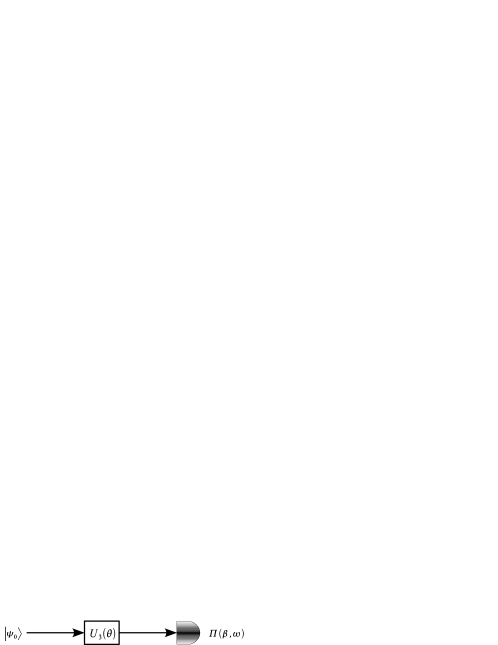
Figure 1: Estimation of qubit gates. The state $\{\rho_{0}\}$ is prepared, then enters the gate described by the unitary $U_{3}(\theta)$ with unknown $\theta$, and finally is detected by a detector described by a two-value POVM.

Upon writing the pure qubit state in the standard way

$$|\psi_{0}\rangle=\cos\frac{\alpha}{2}|0\rangle+e^{i\phi}\sin\frac{\alpha}{2}|1\rangle\>,$$ (9)

where $|0\rangle$ and $|1\rangle$ are the two eigenvectors of $\boldsymbol{\sigma}_{3}$, the parameters $\alpha\in[0,\pi]$ and $\phi\in[0,2\pi]$ uniquely determine $|\psi_{0}\rangle$ and the evolution under the unitary $U_{3}(\theta)$ is straightforward. Next, we perform the measurement described by the two projectors

$$\Pi_{0}(\beta,\omega)=|\Psi(\beta,\omega)\rangle\langle\Psi(\beta,\omega)|\qquad\Pi_{1}(\beta,\omega)={\mathbbm{1}}-\Pi_{0}(\beta,\omega),$$ (10)

where $|\Psi(\beta,\omega)\rangle=\cos\frac{\beta}{2}|0\rangle+e^{i\omega}\sin\frac{\beta}{2}|1\rangle$. The probabilities of the two outcomes are given by $P(0|\theta)\equiv P_{0}(\alpha,\beta,\phi,\omega,\theta)=|\langle 0|U_{\theta}|\psi_{0}\rangle|^{2}$ i.e

$$P(0|\theta) =\frac{1}{2}\left[1+\cos\alpha\cos\beta-\cos(\phi-\omega+\theta)\sin\alpha\sin\beta\right]$$

$$P(1|\theta) =1-P(0|\theta)\>.$$ (11)

The Bayesian a posteriori distribution of Eq. (2) may be written as

$$P(\theta|M)=\frac{1}{N}\>P(0|\theta)^{m_{0}}\>P(1|\theta)^{m_{1}}\>,$$ (12)

where $m_{j}$ is the number of measurements with outcomes $j=0,1$, $m_{0}+m_{1}=M$, in the observed sample. For a large number of measurements $M\gg 1$, we can evaluate $P_{M}(\theta|\theta^{*})$ using Eq. (4) and, in turn, the expectation $\overline{\theta}$ and the variance ${\rm Var}[\theta]$. Upon expanding on $\alpha$ and $\beta$ up to second order one sees that ${\rm Var}[\theta]$ achieves its minimum for the choice $\alpha=\beta=\pi/2$, independently on the value of $\phi$ and $\omega$. This is confirmed by the evaluation of the corresponding Fisher information $G(\theta)$,

$$G(\theta)=\frac{\sin^{2}\alpha\sin^{2}\beta\sin^{2}(\theta+\phi-\omega)}{1-\cos^{2}\alpha\cos^{2}\beta-\cos^{2}(\theta+\phi-\omega)\sin^{2}\alpha\sin^{2}\beta}\>,$$ (13)

which achieves its maximum $G=1$ for $\alpha=\beta=\pi/2$, independently on the value of $\phi$ and $\omega$. Using this results we have:

$$P_{M}(\theta|\theta^{*})=\frac{1}{N}\exp\left[M\left(\cos^{2}\frac{\theta^{*}}{2}\log\cos^{2}\frac{\theta}{2}+\sin^{2}\frac{\theta^{*}}{2}\log\sin^{2}\frac{\theta}{2}\right)\right],$$ (14)

and the variance saturates the van Trees inequality, thus confirming that Bayes estimator is asymptotically efficient. In Fig. 2 we report the ratio $\overline{\theta}/\theta^{*}$ and variance multiplied by ${H_{M}}$ [see Eq. (7)] as a function of the number of measurements. As it apparent from the plots all the curves approach one when the number of measurements increases. In the asymptotic region $H_{M}\simeq MG(\theta)\simeq M$.

\psfrag{thst}{$\overline{\theta}/\theta^{*}$}\psfrag{M}{$M$}\psfrag{V}{${\rm Var}[\theta]{H_{M}}$}\psfrag{300}{300}\psfrag{500}{500}\psfrag{700}{700}\psfrag{1.0000}{1.000}\psfrag{1.0005}{}\psfrag{1.0010}{1.001}\psfrag{1.0015}{}\psfrag{1.0020}{1.002}\psfrag{1.0025}{}\psfrag{1.0030}{1.003}\includegraphics[width=177.78578pt]{rav.eps}

      \psfrag{thst}{$\overline{\theta}/\theta^{*}$}\psfrag{M}{$M$}\psfrag{V}{${\rm Var}[\theta]{H_{M}}$}\psfrag{300}{300}\psfrag{500}{500}\psfrag{700}{700}\psfrag{1.0000}{1.000}\psfrag{1.0005}{}\psfrag{1.0010}{1.001}\psfrag{1.0015}{}\psfrag{1.0020}{1.002}\psfrag{1.0025}{}\psfrag{1.0030}{1.003}\psfrag{M}{$M$}\psfrag{20}{20}\psfrag{40}{40}\psfrag{60}{60}\psfrag{80}{80}\psfrag{100}{100}\psfrag{1.}{1.}\psfrag{1.01}{1.01}\psfrag{1.02}{1.02}\psfrag{1.03}{1.03}\psfrag{1.04}{1.04}\psfrag{1.05}{1.05}\includegraphics[width=177.78578pt]{rvar.eps}

Figure 2: LogLinear plot of $\overline{\theta}/\theta^{*}$ (left) and linear plot of ${\rm Var}[\theta]{H_{M}}$ (right) as a function of the number of measurements $M$ for the estimation of the unitary $U_{3}(\theta)$ and for different values of the true parameter. For both plots the dotted-dashed line is for $\theta^{*}=0.8$, the dashed line is for $\theta^{*}=1.2$ and the solid line is for $\theta^{*}=1.8$.

Notice that the results here reported for $U_{3}(\theta)$ are actually valid for any other unitary gate. This can be seen as follows: any unitary $U_{\boldsymbol{n}}(\theta)=\exp\left(-i\boldsymbol{\sigma}_{n}\theta\right)$ describing rotations around the arbitrary axis $n$ may be written as $U_{\boldsymbol{n}}=OU_{3}(\theta)O^{\dagger}$ where $O$ is the rotation corresponding to the mapping $3\rightarrow{\boldsymbol{n}}$. As a consequence, the optimal measurement corresponds to the projectors $\Pi_{0}^{\prime}=O^{\dagger}|\Psi(0,\omega)\rangle\langle\Psi(0,\omega)|O$, $\Pi_{1}^{\prime}=1-\Pi_{0}^{\prime}$ and the optimal probe is given by $O^{\dagger}|0\rangle$.

A question arises on whether the results reported above may be easily implemented in practice. This concerns the stability of the measurement rather than its precision. The point is the following: Suppose that for some reasons the values of parameters $\alpha$ (probe) $\beta$ (measurement) slightly deviate from the optimal settings. To which extent the overall performances of the procedure are degraded? A convenient way to address this issue is to make a perturbation analysis upon expanding the Fisher information $G(\theta)$ around the optimal settings $\alpha=\beta=\pi/2$ up to second order

$$G(\theta) \simeq 1-\frac{1}{\sin^{2}\theta}\left[(\alpha-\pi/2)^{2}+(\beta-\pi/2)^{2}\right]+2\frac{\cos\theta}{\sin^{2}\theta}(\alpha-\pi/2)(\beta-\pi/2)$$

$$\stackrel{{\scriptstyle\theta\ll 1}}{{\simeq}}1-\frac{1}{\theta^{2}}(\alpha-\beta)^{2}\>.$$ (15)

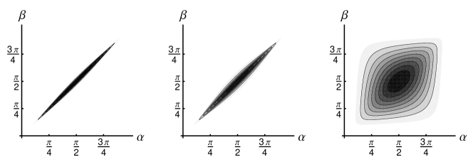
Figure 3: Contour plot of the Fisher information $G(\theta)$ as a function of the probe and measurement parameters $\alpha$ and $\beta$ for three different values of the gate parameter $\theta^{*}=0.05,0.1,1$. Darker areas corresponds to higher values.

Eq. (3.1) shows the quadratic decrease of $G$ out of the optimal setting and, especially for small values of the gate parameter $\theta$, the dramatic effect of a mismatch between the values of $\alpha$ and $\beta$. The latter is well illustrated in Fig. 3 where $G$ as a function of $\alpha$ and $\beta$ is shown for different values of $\theta$. As it is apparent from the plots a mismatch $|\alpha-\beta|\sim\theta$ of the order of the parameter to be estimated is enough to make the whole procedure ineffective. Fortunately, as we will see in Section 3.3, the stability issue may be overcome by using entangled probes and the optimal performances still achieved by a two-qubit probe configuration.

3.2 Monte Carlo simulated experiments

Before addressing stability of the measurement let us compare the asymptotic a posteriori distribution for the gate parameter with the results of Monte Carlo simulated experiments. This is in order to locate the asymptotic region and make quantitative statements on the achievability of the ultimate bounds to precision. We have simulated $M$ repeated measurements using the optimal probe/measurement settings and inserted the resulting values of $m_{j}$, $j=0,1$ in Eq. (12) to obtain the a posteriori distribution for the gate parameter. In Fig. 4 we plot the rescaled variance of this distribution together with the variance of the asymptotic a posteriori distribution of Eq. (14). Remarkably the asymptotic region is achieved after a limited number of runs, thus proving that Bayesian approach may useful in practical applications. In the inset we report the full distribution, both the experimental a posteriori and the asymptotic one, for $M=20$ and $M=500$. Notice that: i) for $M=500$ the a posteriori experimental distribution is already indistinguishable from the asymptotic one and ii) the asymptotic is already unbiased, i.e efficiency has been achieved for a limited number of runs.

\psfrag{P}{\tiny$P(\theta)$}\includegraphics[width=216.81pt]{VarMC.eps}

Figure 4: Rescaled variance (variance multiplied by the generalized Fisher information) of the a posteriori distribution as a function of the number of measurements. Black line is for the asymptotic distribution whereas gray squares are for the experimental one. Inset: asymptotic (dashed line) and experimental (solid line) Bayesian a posteriori distributions for $\theta^{*}=0.6$ as obtained using optimal single-qubit probe and $M=20$ (left) or $M=500$ (right) repeated measurements.

3.3 Estimation via two-qubit entangled probes

An alternative scheme for gate estimation may be designed using entangled states as depicted in Fig. 5. In fact, the use of entanglement may improve estimation [44, 45, 46, 47]. In this section we investigate whether this is the case for the present estimation problem. Basically, the use of entanglement increases the dimension of Hilbert space and thus the number of possible outcomes of a measurement performed on the perturbed signal. The corresponding Fisher information does not increase but the maximum value is achieved for a large class of probe signals. The Bayesian estimator is able to exploit this fact to increase the overall stability of the estimation procedure of the gate parameter.

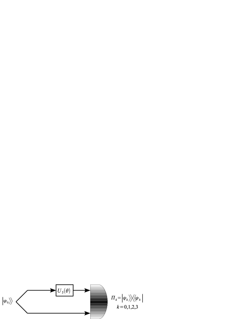
Figure 5: Schematic diagram of parameter estimation by entangled qubit probe: $\{|\psi_{0}\rangle\rangle\}$ is prepared and is subjected to the unitary transformation $U_{\theta}$ on one qubit. Finally, a projective measurement $\{\Pi_{\alpha}\}$ is performed.

In order to see this behavior in practice let us consider the estimation of the parameter of the gate $U_{3}(\theta)$ using a generic pure state of the form

$$|\psi_{0}\rangle\rangle=\frac{1}{\sqrt{2}}\sum_{k=0}^{3}c_{k}|\sigma_{k}\rangle\rangle$$ (16)

where we used the matrix notation for states $|A\rangle\rangle\doteq\sum_{ij}A_{ij}|i\rangle|j\rangle\equiv A\otimes{\mathbbm{I}}|{\mathbbm{I}}\rangle\rangle$. As a measurement we consider the ”Bell” measurement made of the four projectors $\Pi_{k}=\frac{1}{2}|\sigma_{k}\rangle\rangle\langle\langle\sigma_{k}|$, $k=0,1,2,3$, over a set of maximally entangled states. After the evolution under the unitary $U_{3}(\theta)$ the four possible outcomes of the measurements occur with the probabilities

$$P_{0}(\theta) =c_{0}^{2}\cos^{2}\frac{\theta}{2}+c_{3}^{2}\sin^{2}\frac{\theta}{2}\>,\quad P_{1}(\theta)=\left(c_{1}\cos\frac{\theta}{2}-c_{2}\sin\frac{\theta}{2}\right)^{2}\>,$$

$$P_{3}(\theta) =c_{0}^{2}\sin^{2}\frac{\theta}{2}+c_{3}^{2}\cos^{2}\frac{\theta}{2}\>,\quad P_{2}(\theta)=\left(c_{1}\sin\frac{\theta}{2}+c_{2}\cos\frac{\theta}{2}\right)^{2}\>.$$ (17)

The corresponding Fisher information is given by

$$G(\theta)=c_{1}^{2}+c_{2}^{2}+\frac{(c_{0}^{2}-c_{3}^{2})(c_{0}^{4}-c_{3}^{4})\sin^{2}\theta}{(c_{0}^{2}+c_{3}^{2})-(c_{0}^{2}-c_{3}^{2})\cos^{2}\theta}\,$$

and achieves its maximum ($G=1$, $\forall\theta$) for any state with $c_{0}=0$ or $c_{3}=0$. Therefore, having fixed the Bell measurement at the output, a possible deviation in the probe preparations is not degrading the performances of the estimation procedure.

4 Conclusions

In this paper we have analyzed estimation of one-parameter unitary gates for qubit systems. We have addressed Bayesian estimation procedures and compared their performances with the ultimate quantum limits to precision. Bayes estimator is known to be asymptotically unbiased, but for practical implementation is of interest to evaluate quantitatively how many measurements are needed to achieve the asymptotic region. To this aim, after the evaluation of the asymptotic a posteriori distribution for the gate parameter, we have compared it to the distribution obtained by Monte Carlo simulated experiments and full Bayesian analysis and shown that asymptotic optimality of Bayes estimator is achieved after a limited number of runs. We have also addressed the issue of stability, i.e the robustness of the optimal settings against fluctuations of the probe and measurement parameters. It has been shown that the use of entanglement is useful to improve stability. More explicitly, we have shown that, although the Fisher information does not increase, its maximum value is achieved for a large class of probe signals, thus making the procedure more robust and increasing the overall stability of the estimation procedure.

References

References

- [1] C. W. Helstrom, Quantum Detection and Estimation Theory (Academic Press, New York, 1976).
- [2] A. S. Holevo, Probabilistic and Statistical Aspects of Quantum Theory (North-Holland, Amsterdam, 1982).
- [3] I. L. Chuang and M. A. Nielsen, J. Mod. Opt. 44, 2455 (1997).
- [4] J. F. Poyatos, et al., Phys. Rev. Lett. 78, 390 (1997).
- [5] S. L. Braunstein and C. M. Caves, Phys. Rev. Lett. 72, 3439 (1994).
- [6] A. S. Holevo, Prob. Theory Appl. 49, 207 (2004).
- [7] R. D. Gill and S. Massar, Phys. Rev. A 61, 042312 (2000).
- [8] O. E. Barndorff-Nielsen and R. D. Gill, J. Phys. A 30, 4481 (2000).
- [9] A. Fujiwara and H. Nagaoka, Phys. Lett. A 201, 119 (1995).
- [10] M. G. A. Paris, Phys. Rev. A 53, 2658 (1996).
- [11] S. L. Braunstein and C. M. Caves, in Fundamental problems in quantum theory, Vol. 755 of Annals of the New York Academy of Sciences, edited by D. Greenberger and A. Zellinger (New York Academy of Sciences, New York, 1995), pp. 786-797.
- [12] S. L. Braunstein and C. M. Caves in Quantum communication and Measurement, edited by V. P. Belavkin, O. Hirota, and R. L. Hudson (Plenum, New York, 1995), pp. 21-30.
- [13] S. L. Braunstein, C. M. Caves, and G. J. Milburn, Ann. Phys. (N. Y.) 247, 135 (1996).
- [14] G. M. D’Ariano, L. Maccone, M. G. A. Paris, J. Phys. A, 34, 93 (2001).
- [15] K. Banaszek, G.M. D’Ariano, M.G.A. Paris, and M.F. Sacchi, Phys. Rev. A 61 10304 (2000).
- [16] S. Boixo, et al., Phys. Rev. Lett. 98, 090401 (2007).
- [17] E. Knill, G. Ortiz, and R. D. Somma, Phys. Rev. A 75, 012328 (2007).
- [18] V. Giovannetti, S. Lloyd, and L. Maccone, Phys. Rev. Lett. 96, 010401 (2006).
- [19] M. G. A. Paris and J. Řeháček, Quantum State Estimation, Lect. Notes Phys. 649 (2004).
- [20] D. F. V. James, P. G. Kwiat, W. J. Munro, and A.G. White, Phys. Rev. A 64, 052312 (2001).
- [21] S. Cialdi, F. Castelli, I. Boscolo, M. G. A. Paris, Appl. Opt. 47, 1832 (2008).
- [22] A. M. Childs et al., Phys. Rev. A 64 012314 (2001).
- [23] M. W. Mitchell et al., Phys. Rev. Lett. 91 120402 (2003).
- [24] G. M. D’Ariano, P. Lo Presti, Phys. Rev. Lett. 91 047902 (2003).
- [25] J. L O’Brien et al., Phys. Rev. Lett. 93, 080502 (2004).
- [26] S. H. Myrskog et al., Phys. Rev. A 72 013615 (2005).
- [27] H. L. Van Trees and K. L. Bell, Bayesian Bounds for Parameter Estimation and Nonlinear Filtering/Tracking, (IEEE Press and Wiley Interscience, 2007).
- [28] H. Cramer, Mathematical Methods of Statistics, (Princeton University Press, 1946).
- [29] C. R. Rao, Proc. Cambridge Phil. Soc., 43, 280 (1946).
- [30] H. V. Poor, An Introduction to Signal Detection and Estimation (New York, Wiley, 1973).
- [31] T. M. Cover and J. A. Thomas, Elements of Information Theory (Wiley, New York, 2006).
- [32] M. Hayashi in Quantum Communication, Computing and Measurement, edited by O. Hirota, A. S. Holevo, and C. M. Caves, (Plenum Publishing, New York, 1997).
- [33] M. Hotta and M. Ozawa, Phys. Rev. A 70, 022327 (2004).
- [34] E. L. Lehmann and G. Casella, Theory of Point Estimation, 2nd.ed (Springer, New York, 1994).
- [35] H. L. van Trees, Detection, Estimation, and Modulation Theory I, (Wiley, New York, 2001).
- [36] M. P. Schützenberger, Bull. Amer. Math. Soc. 63, 142 (1957).
- [37] Z. Hradil et al., Phys. Rev. Lett. 76, 4295 (1996).
- [38] L. Pezze et al., Phys. Rev. Lett. 99, 223602 (2007).
- [39] J. M. Bernardo and A. F. M. Smith, Bayesian Theory (Wiley, Chichester, 1994).
- [40] D. Malakoff, Science 286, 1460 (1990).
- [41] Z. Hradil, Phys. Rev. A 51, 1875 (1995).
- [42] Z. Hradil et al., Phys. Rev. Lett. 76, 4295 (1996).
- [43] L. Le Cam, Asymptotic Methods in Statistical Decision Theory (Springer, New York, 1986).
- [44] A. Fujiwara, Phys. Rev. A 63, 042304 (2001).
- [45] G. M. D’Ariano, P. Lo Presti, M. G. A. Paris, Phys. Rev. Lett. 87, 3439 (2001).
- [46] G. M. D’Ariano, M. G. A Paris, P. Perinotti, J. Opt. B, 4, S277 (2002).
- [47] G. M. D’Ariano, M. G. A. Paris, P. Perinotti, Phys. Rev A 65 062106 (2002).
- [48] Cut-throat savings Nature 455, 835 October (2008).