ILC Beam Energy Measurement by means of Laser Compton Backscattering

N. Muchnoi¹, H.J. Schreiber² and M. Viti²

Abstract

A novel, non-invasive method of measuring the beam energy at the International Linear Collider is proposed. Laser light collides head-on with beam particles and either the energy of the Compton scattered electrons near the kinematic endpoint is measured or the positions of the Compton backscattered $\gamma$-rays, the edge electrons and the unscattered beam particles are recorded. A compact layout for the Compton spectrometer is suggested. It consists of a bending magnet and position sensitive detectors operating in a large radiation environment. Several options for high spatial resolution detectors are discussed. Simulation studies support the use of an infrared or green laser and quartz fiber detectors to monitor the backscattered photons and edge electrons. Employing a cavity monitor, the beam particle position downstream of the magnet can be recorded with submicrometer precision. Such a scheme provides a feasible and promising method to access the incident beam energy with precisions of $10^{-4}$ or better on a bunch-to-bunch basis while the electron and positron beams are in collision.

1 Introduction

A full exploitation of the physics potential of the International $e^{+}e^{-}\>$Linear Collider (ILC) must aim to control the absolute incoming beam energy, $E_{b}$, to an accuracy of $10^{-4}$ or better. Precise measurements of $E_{b}$ is a critical component to measuring the center-of-mass energy, $\sqrt{s}$, as it sets the overall energy scale of the collision process. Good knowledge of $E_{b}$, respectively, $\sqrt{s}$ had always been a tremendous advantage for performing precise measurements of particle masses and the differential dependence of the luminosity, $d{\cal{L}}/d\sqrt{s}$. At circular machines, for example at the Large Electron Positron Collider (LEP), beam energy determination using resonant depolarization allowed an exquisite measurement of the $Z$ boson mass, $M_{Z}$, to an uncertainty of 2 MeV or 23 parts per million (ppm). At the ILC, however, the resonance depolarization technique cannot be applied and different methods have to be employed.

A beam position monitor-based magnetic spectrometer is considered to be a well established and promising device to achieve this goal [1]. By means of this method, the energy is determined by measuring the deflection angle of the particle bunches utilizing beam position monitors (BPMs) and the field integral, $B\equiv\int Bd\ell$, mapped to high resolution. The performance of such a spectrometer has been demonstrated at LEP at CERN, where an in-line spectrometer with button monitors was successfully operated to cross-check the energy scale for W mass measurements [2]. A relative error on $\sqrt{s}$ of 120-200 ppm has been achieved, thanks to careful cross-calibrations using resonant depolarization. While the primary beam energy determination was based on the NMR magnetic model, its validity was, after corrections for different sources of systematic errors, verified by three other methods: the flux-loop, which is sensitive to the bending fields of all dipole magnets of LEP, a BPM-based spectrometer and an analysis of the variation of the synchrotron tune with the total RF voltage. At SLAC, a synchrotron radiation-stripe (WISRD) based bend angle measurement in the extraction line of the $e^{+}e^{-}\>$interaction point (IP) was performed to access $\sqrt{s}$ [3]. The results obtained were, however, subject to corrections by 46$\pm$25 MeV, i.e. by 500 ppm, utilizing the precise value of $M_{Z}$ from LEP. All these trials to measure the energy evidently emphasize the following lesson: more than one technique should be applied for precise $\sqrt{s}$ determinations and cross-calibration of the absolute energy scale is mandatory. In the past, novel suggestions, see e.g. [4], were proposed for the ILC and some of them were evaluated in detail. Within the next years some consensus should, however, be arrived at as to which methods are most promising of being complementary to the canonical BPM-based spectrometer technique.

In this note we propose a new non-destructive approach to perform beam energy measurements using Compton backscattering of laser light by beam particles. The energy at the kinematic endpoint (edge) of the Compton electrons depends on $E_{b}$, and its direct measurement provides the beam energy. Alternatively, recording the positions of the Compton backscattered photons and the edge electrons together with the position of the unscattered beam particles allows to infer the primary beam energy with high precision.

Compton backscattering experiments have been performed with great success at circular low-energy accelerators. At the Taiwan Light Source [5], the beam energy of 1.3 GeV was determined with an uncertainty of 0.13%. At BESSY I and II [6] with 800 MeV, respectively, 900 or 1700 MeV electron energy, $E_{b}$ was found to be in very good agreement with the resonant depolarization values, and at Novosibirsk [7] an accuracy of 60 keV was obtained for beam energies between 1.7 and 1.9 GeV. In all these experiments, beam particles were collided head-on with photons from a $CO_{2}$ laser. The maximum energy of the forward going Compton $\gamma$-rays was measured with high-purity germanium detectors and converted into the central primary beam energy.

This method, however, is not practicable at the ILC since precise $E_{b}$ measurements require collective and accurate information on Compton backscattered particles using large event rates per bunch crossing. The selection of the photon with highest energy and its precise measurement out of a large number of $\gamma$-rays cannot be performed. In particular, within bunch crossings of picosecond duration a calorimetric approach (with demanding calibration performance) to access the maximum $\gamma$-ray energy is unable to resolve the individual backscattered photons. Therefore, the method proposed for the linear collider is different and can be summarized as follows: after crossing of laser light with beam electrons, a bending magnet separates the forward collimated Compton photons and electrons as well as the non-interacting beam particles such that downstream of the dipole high spatial resolution detectors measure the positions of the backscattered photons and the edge electrons, i.e. of electrons with smallest energy or largest deflection. If these measurements are either combined with the magnetic field integral or with the position of the unscattered beam particles, the beam energy can be inferred.

At the ILC, laser Compton backscattering off beam particles is also suggested to probe other properties of the beam, such as the transverse profile [8] or the degree of polarization [9].

In the past, laser backscattered $\gamma$-rays off relativistic electrons were employed as a highly promising alternative of producing intense and directional quasi-monochromatic (polarized) photon beams to investigate photonuclear reactions [10], to calibrate detectors or to record medical images.

The paper is organized as follows. Sect.2 describes the basic properties of the Compton scattering process, emphasizing features which are relevant for $E_{b}$ determinations. In Sect.3 an overview of the proposed method is presented. Two schemes to perform beam energy measurements are suggested and precisions achievable are discussed. This will be followed by a setup proposal, a layout of the vacuum chamber, a suitable dipole suggestion, a possible laser system and detector options to measure the photon and edge electron positions as well as that of the unscattered beam. Simulation studies support the feasibility and reliability of the concepts proposed. Processes beyond the Born approximation in the laser crossing region such as nonlinear effects, multiple scattering, higher order QED contributions and pair production background are also discussed. This is followed by a discussion of potential sources of errors affecting the measurement of $E_{b}$. Possible locations of a Compton energy spectrometer within the ILC beam delivery system [11] are summarized at the end of Sect.3. Sect.4 contains the summary and conclusions.

2 The Compton Scattering Process

Feenberg and Primakoff [12] proposed in 1948 the kinematics formula for the two-to-two Compton scattering process

$$e+\gamma\rightarrow e^{\prime}+\gamma^{\prime}~{},$$ (1)

which is shown in Fig. 1 in the lab frame. The initial photon and electron energies are expressed as $E_{\lambda}$ and $E_{b}$, respectively, while the energy of the backscattered photon is expressed as $E_{\gamma}$ and that of the electron as $E_{e}$. $\theta_{\gamma}$ is the scattering angle between the initial electron and the laser direction. The angle $\alpha$, not shown in Fig. 1, is defined between the incident electron and the laser direction.

Throughout this study, the convention is used where the positive z-axis is defined to be the direction of the incident beam, the x-axis lies in the horizontal or bending plane and the y-axis points to the vertical direction such that a right-handed coordinate system is obtained.

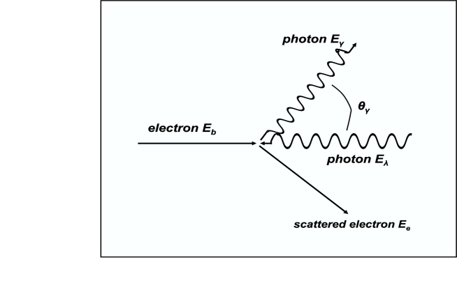
Figure 1: The kinematics of Compton scattering in the lab frame. The energies of the colliding electron and laser photon are denoted as $E_{b}$ and $E_{\lambda}$, respectively. $\theta_{\gamma}$ is the scattering angle between the initial electron and final state photon. The angle $\alpha$ is not shown.

2.1 Compton Scattering Cross Section

In order to calculate the cross section for Compton scattering (in Born approximation) we start from the matrix element which involves two Feynman diagrams as shown in Fig. 2.

Figure 2: Leading order Feynman diagrams contributing to the Compton cross section.

Since the ILC is also planned to operate with polarized electrons/positrons, it is advantageous to consider the most general case by including possible spin-states of the incident particles.

In the lab frame, the Compton kinematics are characterized by the dimensionless variable

$$x=\frac{4E_{b}E_{\lambda}}{m^{2}}\cdot\cos^{2}(\alpha/2)\sim\frac{4E_{b}E_{\lambda}}{m^{2}}$$ (2)

and the normalized energy variable

$$y=1-\frac{E_{e}}{E_{b}}=\frac{E_{\gamma}}{E_{b}}~{}.$$ (3)

Applying QED Feynman rules, the spin-dependent differential cross section is after summing over the non-interesting spin and polarization states of the final state particles

$$\frac{d\sigma}{dy}=\frac{2\sigma_{0}}{x}[\frac{1}{1-y}+1-y-4r(1-r)+P_{e}\lambda rx(1-2r)(2-y)]~{},$$ (4)

where $P_{e}$ is the initial electron helicity (-1 $\leq P_{e}\leq$ +1), $\lambda$ the initial laser helicity (-1 $\leq\lambda\leq$ +1), $r=\frac{y}{x(1-y)}$ and $\sigma_{0}=\pi r^{2}_{0}$ = 0.2495 barn, with $r_{0}$ the classical electron radius.

Fig. 3 shows the unpolarized Compton cross section as a function of the beam energy for three laser energies, $E_{\lambda}$ = 0.117, 1.165 and 2.33 eV. At all incident energies,

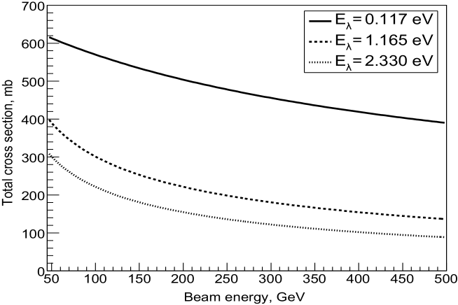
Figure 3: Compton backscattering cross section versus beam energy for three laser energies.

the $CO_{2}$ laser with $E_{\lambda}$ = 0.177 eV provides the largest cross sections, while the $Nd:YAG$ laser (with $E_{\lambda}$ = 1.165 or 2.33 eV) cross sections are significantly smaller. For example, at 250 GeV the $CO_{2}$ cross section is more than two times larger than the $Nd:YAG$ laser values.

We also note that for the polarization configuration $P_{e}\lambda$ = -1, the cross section close to the electron’s kinematic endpoint is enhanced by typically a factor two, while for the configuration $P_{e}\lambda$ = +1 the edge Compton cross section vanishes. This behavior is shown in Fig. 4, where for the three cases, $P_{e}\lambda$ = -1, $P_{e}\lambda$ = +1 and unpolarized, the cross section is plotted as a function of the scattered electron energy for the infrared $Nd:YAG$ laser at 250 GeV. For polarized electrons the favored spin configuration $P_{e}\lambda$ = -1 can always be achieved by adjusting the laser helicity $\lambda$.

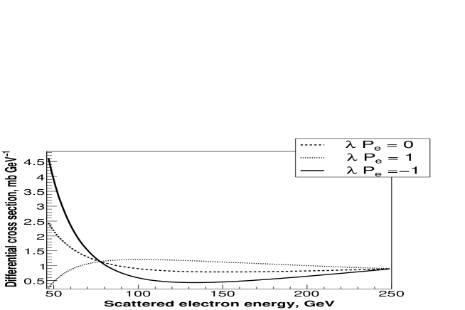
Figure 4: Compton backscattering cross section for three polarization configurations versus scattered electron energy for an infrared $Nd:YAG$ laser at 250 GeV.

2.2 Properties of the Final State Particles

After scattering, the angles of the Compton scattered photons and electrons relative to the incoming beam direction are

$$\theta_{\gamma}=\frac{m}{E_{b}}\cdot\sqrt{\frac{x}{y}-(x+1)}~{},~{}~{}~{}~{}~{}~{}\theta_{e}=\theta_{\gamma}\cdot\frac{y}{1-y}~{},$$ (5)

and the $\gamma$-ray emerges with an energy of

$$E_{\gamma}=E_{\lambda}\cdot\frac{1-\beta\cos\alpha}{1-\beta\cos\theta_{\gamma}+\frac{E_{\lambda}(1-\cos(\theta_{\gamma}-\alpha))}{E_{b}}}$$ (6)

at small angle $\theta_{\gamma}$, with $\beta$ the beam electron velocity divided by the speed of light and $\alpha$ the angle between the laser light and the incident beam. $E_{\gamma}$ ranges from zero to some maximum value

$$E_{\gamma,max}=\frac{E_{b}^{2}}{E_{b}+\frac{m^{2}}{4\omega_{0}}}~{},~{}~{}~{}~{}~{}~{}~{}\omega_{0}=E_{\lambda}\cdot\cos^{2}(\alpha/2)~{}.$$ (7)

Fig. 5 illustrates the energy and x-position of the scattered photons at a plane located 50 m downstream of the Compton IP for three laser energies, $\alpha$ = 8 mrad and $E_{b}$ = 250 GeV.

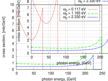
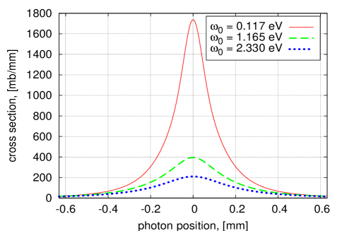
Figure 5: Energy and x-position of backscattered photons for three laser energies, $\alpha$ = 8 mrad and $E_{b}$ = 250 GeV. The photon position is determined at a plane 50 m downstream of the Compton IP.

According to eq.(7), $\gamma$-rays with highest energy travel exactly forward.

The energy of the Compton electrons is determined by energy conservation. The maximum energy of the Compton photon is related to the minimum (or edge) energy of the scattered electron, $E_{edge}$, via

$$E_{edge}=E_{b}+E_{\lambda}-E_{\gamma,max}=\frac{E_{b}}{1+\frac{4E_{b}\omega_{0}}{m^{2}}}~{},$$ (8)

if $E_{\lambda}$ is neglected. The electron scattering angle $\theta_{e}$, given in eq.(5), approaches zero as $\theta_{\gamma}$ becomes smaller. Thus, in the region of smallest electron energy, the region of our interest, both the scattered electrons and photons are generated at very small angles.

Fig. 6 shows the unpolarized Compton cross section as a function of the scattered electron energy for three laser energies at 250 GeV.

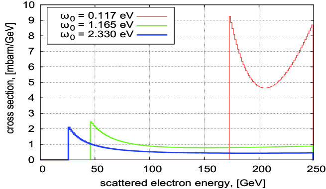
Figure 6: Compton backscattering cross section versus electron energy for three laser wavelengths at 250 GeV.

The $CO_{2}$ laser (with an energy of 0.177 eV) provides the most pronounced edge cross section, while the $Nd:YAG$ laser (with $\omega_{0}$ = 1.165 or 2.33 eV) cross sections are significantly smaller. At the electron’s edge position, $E_{edge}$, both $Nd:YAG$ lasers provide cross sections of similar size, with edge energy values relatively close to each other.

Since one of the proposed methods for measuring the beam energy utilizes the variation of the edge energy on $E_{b}$, see eq.(8), we present in Fig. 7 the edge energy dependence on $E_{b}$ for three laser wavelengths. As can be seen, the derivative $dE_{edge}/dE_{\lambda}$ or the slope, respectively, sensitivity of the edge energy on $E_{b}$ decreases with increasing laser energy. In particular, for an infrared or green laser, the sensitivity is very small, which suggests to employ lasers with large wavelengths, such as a $CO_{2}$ laser, for this method.

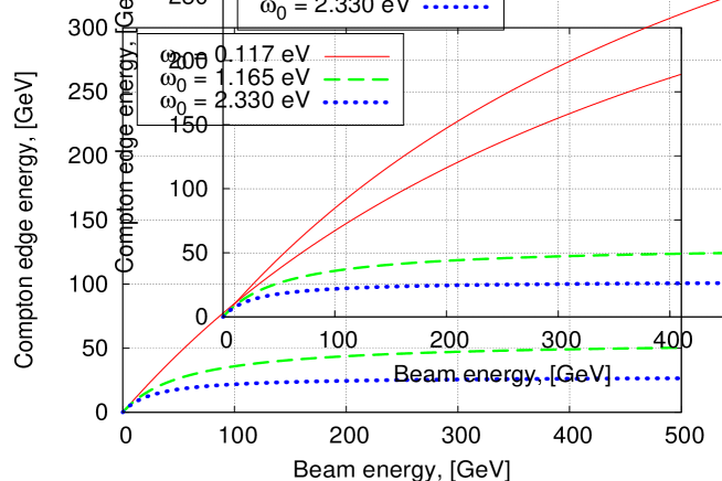
Figure 7: Edge energy of Compton electrons as a function of $E_{b}$ for a $CO_{2}$, infrared and green laser.

From these discussions we can draw first conclusions relevant for beam energy determinations:

• the electron edge energy, $E_{edge}$, depends on the beam energy (eq.(8)), on which one of the proposals for measuring $E_{b}$ relies;

• if this method will be utilized, low energy lasers are advantageous because of large Compton cross section and high endpoint $E_{b}$ sensitivity;

• backscattered electrons and photons are predominantly scattered in the direction of the incoming beam;

• photons associated with the edge electrons have largest energy and point towards $\theta_{\gamma}$ = 0;

• the unpolarized Compton cross section peaks at $E_{edge}$ which results in beam energy determinations with small statistical errors;

• for polarized electrons, choose the polarization configuration $P_{e}\lambda$ = -1; the unfavored configuration $P_{e}\lambda$ = +1 spoils any $E_{b}$ determination.

So far, the cross section formulas and backscattered particle properties were discussed in Born approximation. Possible modifications due to multiple scattering, $e^{+}e^{-}\>$pair background, higher order corrections and nonlinear effects were partially discussed in [13] and are further studied in Sect.3.10.

2.3 Luminosity of Compton Scattering

To turn from cross sections to number of Compton events, the luminosity of $e^{-}\gamma$ collisions has to be known. In principle, there are two cases to consider: collisions of beam electrons with a continuous laser or a pulsed laser that matches the pattern of the incident electron bunches at the ILC. In the following we assume that the particle densities in both beams are of Gaussian-shape.

• Continuous laser

The luminosity of a continuous laser with a pulsed electron of round transverse profile ($\sigma_{x}=\sigma_{y}$) can be expressed as [14]

$$L_{cont}=\frac{1+\cos\alpha}{\sqrt{2\pi}\sin\alpha}\cdot\frac{N_{e}P_{L}}{cE_{\lambda}}\cdot\frac{1}{\sqrt{\sigma_{x\gamma}^{2}+\sigma_{xe}^{2}}}~{},$$ (9)

where $N_{e}$ is the number of electrons per bunch, $P_{L}$ the average power of the laser with energy $E_{\lambda}$, and $\alpha$ the crossing angle of the two beams. The horizontal beam sizes are characterized by $\sigma_{x\gamma}$ and $\sigma_{xe}$. Although the ILC beam is not actually round as assumed, it does not matter here, since usually $\sigma_{x\gamma}>\sigma_{xe}$.

If the crossing angle $\alpha$ becomes zero, the expression for the luminosity explodes. If, however, the electron bunch is completely contained within the laser spot, as is normally the case, the luminosity is restricted by the finite laser beam emittance $\varepsilon_{\gamma}$

$$L_{cont,max}=\frac{N_{e}P_{L}}{cE_{\lambda}}\cdot\frac{1}{\varepsilon_{\gamma}}~{}.$$ (10)

For a perfect laser, the best possible emittance is limited by the laws of optics and depends on the wavelength $\varepsilon_{\gamma}=\lambda/4\pi$. The associated maximum possible luminosity is then determined as

$$L_{cont,max}=4\pi\cdot\frac{N_{e}P_{L}}{hc^{2}}~{},$$ (11)

where $h$ is the Planck constant and $c$ the speed of light.

• Pulsed laser

For a pulsed laser, the luminosity per bunch crossing is [14]

$$L_{pul}=N_{\gamma}\cdot N_{e}\cdot g~{},$$ (12)

with $N_{\gamma}$ the number of photons per laser pulse and $N_{e}$ the number of electrons per bunch. With no loss of generality, the geometrical factor $g$ for vertical beam crossing is well approximated by

$$g=\frac{\cos^{2}\alpha/2}{2\pi}\cdot\frac{1}{\sqrt{\sigma^{2}_{xe}+\sigma^{2}_{x\gamma}}}\cdot\frac{1}{\sqrt{(\sigma^{2}_{ye}+\sigma^{2}_{y\gamma})\cos^{2}(\alpha/2)+(\sigma^{2}_{ze}+\sigma^{2}_{z\gamma})\sin^{2}(\alpha/2)}}~{},$$ (13)

where $\alpha$ is the crossing angle and the transverse laser profile is assumed to be constant. Note that the vertical, respectively, longitudinal bunch sizes $\sigma_{y\gamma}$, $\sigma_{ye}$ and $\sigma_{z\gamma}$, $\sigma_{ze}$ of the interacting beams contribute.

For small $\alpha$ and transverse dimensions of the electron beam compared to the laser focus, i.e. $\sigma_{xe}<\sigma_{x\gamma}$ and $\sigma_{ye}<\sigma_{y\gamma}$, which is generally valid at the crossing point, the geometrical factor reduces to

$$g=\frac{1}{2\pi\sigma_{x\gamma}\sigma_{y\gamma}~{}\sqrt{1+(0.5\alpha\cdot\sigma_{z\gamma}/\sigma_{y\gamma})^{2}}}~{}.$$ (14)

For given $\sigma_{x\gamma}$, $\sigma_{y\gamma}$ of the laser focus, the bunch related luminosity reaches a maximum for small crossing angles and short laser pulses:

$$L_{pul,max}=\frac{N_{\gamma}\cdot N_{e}}{2\pi\sigma_{x\gamma}\sigma_{y\gamma}}~{}.$$ (15)

This formula is very similar to the expression given for the luminosity of the colliding beams at the physics $e^{+}e^{-}$ interaction point.

3 Overview of the Experiment

3.1 Basic Experimental Conditions

Within the so-called single-event regime, individual Compton events originate from separate accelerator bunches. As was realized in experiments at storage rings [5, 6, 7], recording the maximum energy of the scattered photons out of many events enables to infer the beam energy.

The experimental conditions at the ILC with large bunch crossing frequencies and high particle intensity require to operate with short and intense laser pulses so that high instantaneous event rates are achieved. As a result, the detector signals for a particular bunch crossing correspond to a superposition of multiple events. In such a regime, single photon detection cannot be realized and the signal will likely be an energy weighted integral over the entire photon spectrum. The number of Compton interactions should, however, be adjusted such that neither the incident electron beam will be disrupted nor the Compton event rate degrades the performance of the detectors.

It is also worth to note that it might be useful for e.g. calibration purposes to operate occasionally in the single-event regime, either with reduced pulse power of the laser or even with CW lasers.

The concept of a possible Compton energy spectrometer is shown in Fig. 8. Downstream of the laser crossing point, a bending magnet is positioned which is followed by a dedicated particle detection system. This system has to provide precise position information of the backscattered photons and electrons close to the edge and, employing an alternative method, the position of the unscattered beam.

Figure 8: Scheme of the proposed energy spectrometer based on Compton backscattering.

The vacuum chamber between the Compton IP and the detector plane needs some special design to accommodate simultaneously the trajectories of the photons, the degraded backscattered electrons and the non-interacting beam particles. In order to ensure large luminosity, the crossing angle should be very small and, for reasons of reduced radiation exposure to the optical elements above and below the electron beamline, vertical beam crossing is suggested.

The dipole magnet located about 3 m downstream of the crossing point separates the particles coming from the IP into the undeflected backscattered photons, the Compton electrons and the beam particles with smallest bending angle. The B-field integral should be scaled to the primary beam energy, so that beam particle deflection occurs always at 1 mrad. Thus, one BPM with fixed position is sufficient to record the beamline position at all energies. The photon detector is located in the direction of the original beam, while the electron detector has to be adjusted horizontally according to Compton scattering kinematics and the magnetic field.

The laser system should consist on a pulsed laser, while a continuous laser might only be occasionally used for special tasks such as detector calibration or operation at the $Z$-pole. At ILC energies Compton scattering with typical continuous lasers in the 1-10 Watt range takes some fraction of an hour to collect enough statistics for precise $E_{b}$ determination. Thus, in order to perform bunch related energy measurements the default laser system should be a pulsed laser with a pattern that matches the peculiar pulse and bunch structure of the ILC, i.e. at 250 GeV an inter-bunch spacing of $\sim$300 ns within 1 ms long pulse trains at 5 Hz. In order to collect typically $10^{6}$ Compton events per bunch crossing, the pulse power of the $CO_{2}$ laser should be about 5 mJ , while for an infrared laser with $E_{\lambda}$ = 1.165 eV, the smaller Compton cross section will be partially compensated by a smaller spot size, a power of 30 mJ is needed. A laser in the green wavelength range with 2.33 eV photon energy requires a pulse power of 24 mJ for $10^{6}$ Compton interactions. For $Z$-pole running, the laser power can be somewhat smaller, but it has to be increased for 1 TeV runs. Since at present lasers with such exceptional properties are not commercially available, R&D is needed to achieve the objectives, see e.g. [16, 17, 18].

To maximize the $e\gamma$ luminosity, the crossing angle $\alpha$ should be small, in our case 8-10 mrad, and the laser spot should be larger than the horizontal electron beam size, which is expected to be in the range of 10-50 $\mu$m within the beam delivery system (BDS). For a well aligned laser it should be practicable to keep possible horizontal and vertical relative displacements of the electron and laser beams small enough, so that permanent overlap is ensured even in cases of beam position jitter.

The choice of a suitable laser system is determined by several constraints. Basically, lasers with large wavelengths such as a $CO_{2}$ laser with $\lambda=10.6~{}\mu$m provide high event rates due to large Compton cross sections and best beam energy sensitivity of the endpoint position, see Fig. 7. Lasers in the infrared region such as $Nd:YAG$ or $Nd:YLF$ lasers, however, provide at present a better reliability, in particular with respect to the bunch pattern and pulse power [18] and would relax geometrical constraints of the spectrometer setup due to substantially smaller electron edge energies, see Fig. 6. Green laser R&D is ongoing within the ILC community to develop laser-wire diagnostics [8] and high energy polarimeters [9].

Fig. 9 shows for three wavelengths and a particular setup (with a B-field of 0.28 T and a detector 25 m downstream of the magnet) the horizontal or x-position of the Compton electrons. The position of electrons with highest energy coincides with the beamline position independent of the laser, whereas the positions of the edge electrons with largest deflection are very distinct. They are smaller for larger laser wavelength. For a $CO_{2}$ laser at 45.6 GeV, the edge electrons are separated by only 2.2 mm from the beamline, while they are displaced from the backscattered $\gamma$-rays by about 2.6 cm. Such space conditions would prevent the use of a $CO_{2}$ laser for $Z$-pole calibration runs. An increased B-field and/or a larger drift distance could somewhat relax the situation.

Lasers in the green or infrared wavelength region have some disadvantages. They provide smaller Compton cross sections and hence smaller event rates, which might only be

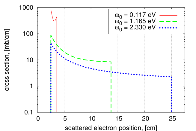
Figure 9: Scattered electron positions for $E_{b}$ = 250 GeV, a B-field of 0.28 T and three laser energies. The detector is placed 25 m downstream of the spectrometer magnet.

compensated by higher laser power and/or smaller but limited spot sizes. Also, the smaller sensitivity of the edge position on $E_{b}$ (Fig. 7) and the generation of additional background at large $\sqrt{s}$ due to $e^{+}e^{-}\>$pairs from Breit-Wheeler processes might disfavor their application. As soon as the variable x of eq.(2) exceeds 4.83, which is for example the case at 250 GeV and a green laser, $e^{+}e^{-}\>$pair production is kinematically possible. Whether this source of background is tolerated will be studied in Sect.3.10. Some of the disadvantages discussed are of less relevance if an alternative method, called method B in the following, will be employed for beam energy determination.

3.2 Method A

One approach to measure the ILC beam energy by Compton backscattering relies on precise electron detection at the kinematic endpoint. In particular, endpoint or edge energy measurements are performed, from which via eq.(8), the beam energy is accessible. In particular, the Compton edge electrons are momentum analyzed by utilizing a dipole magnet and recording their displacement downstream of the magnet.

The conceptual detector design consists of a component to measure the center-of-gravity of the Compton backscattered $\gamma$-rays and a second one to access the position of the edge electrons. The distance $D$ of the center-of-gravity to the edge position and the well known drift space $L$ between the dipole and the detector determine the bending angle $\Theta$ of the edge electrons, which, together with the B-field integral, fixes the energy of the edge electrons:

$$E=\frac{c\cdot e}{\Theta}\int\limits_{magnet}Bdl~{}.$$ (16)

Here, c is the speed of light and e the charge of the particles. Thus, for sufficient large drift space the edge electrons are well separated from the Compton scattered photons which pass the magnet undeflected.

A demanding aspect of this approach is the precision for the displacement, $\Delta D$, which is related to the beam energy uncertainty as

$$\frac{\Delta E_{b}}{E_{b}}=(1+\frac{4E_{\lambda}E_{b}}{m^{2}})\sqrt{\left(\frac{\Delta B}{B}\right)^{2}+\left(\frac{\Delta L}{L}\right)^{2}+\left(\frac{\Delta D}{D}\right)^{2}}~{}.$$ (17)

This relation follows from eqs.(7), (8) and

$$\frac{\Delta E_{edge}}{E_{edge}}=\frac{E_{edge}}{E_{b}}\cdot\frac{\Delta E_{b}}{E_{b}}~{}$$ (18)

as well as

$$\left(\frac{\Delta E_{edge}}{E_{edge}}\right)^{2}=\left(\frac{\Delta\Theta}{\Theta}\right)^{2}+\left(\frac{\Delta B}{B}\right)^{2}~{}$$ (19)

together with $D=\Theta\cdot L$ from the geometry of the setup. Synchrotron radiation effects on $\Delta E_{b}/E_{b}$, estimated to be significantly smaller than any term in (17), were omitted.

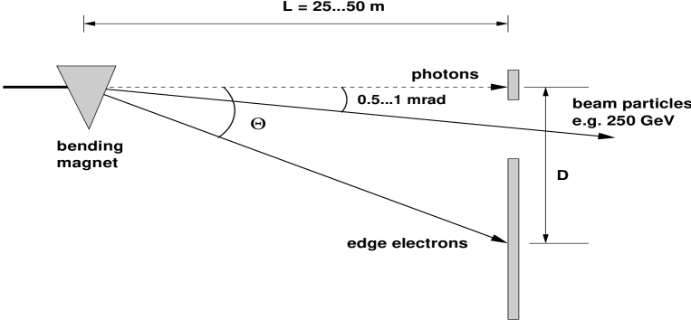
Figure 10: Sketch of an experimental layout.

One notices from eq.(17) that smallest beam energy uncertainties are achievable for lasers with large wavelengths, such as a $CO_{2}$ laser.

Assuming a relative error of the field integral of $2\cdot 10^{-5}$ and for $\Delta L/L=5\cdot 10^{-6}$, $\Delta E_{b}/E_{b}$ values as a function of $\Delta D$ are displayed in Fig. 11 for three laser options at 250 GeV. Drift distances of either 25 or 50 m and 0.5 or 1.0 mrad for the bend angle were assumed.

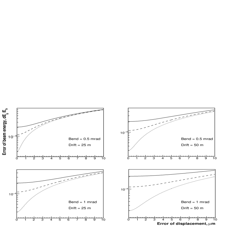
Figure 11: Beam energy uncertainty as a function of the edge electron displacement error for the green laser (full curve), the infrared laser (dashed curve) and the $CO_{2}$ laser (dotted curve) for two values of drift space and bending angle. The beam energy is 250 GeV.

Clearly, in order to achieve a precision of $\Delta E_{b}/E_{b}=10^{-4}$, $\Delta D$ has to be smaller than a fraction of a micrometer for a green laser, even for a drift distance of 50 m and 1 mrad bending power. In contrast, a $CO_{2}$ laser allows for less stringent demands of the displacement error: $\Delta D$ might be in the order of few micrometers.

Since the displacement is determined by the center-of-gravity of the recoil $\gamma$-rays and the position of the electron edge, the displacement error $\Delta D$ is given by the corresponding uncertainties as $\sqrt{\Delta X_{\gamma}^{2}+\Delta X_{edge}^{2}}$. The edge position accuracy $\Delta X_{edge}$ can be estimated as

$$\Delta X_{edge}=\sqrt{\frac{2\cdot\sigma_{X_{edge}}}{\frac{dN}{dx}(X_{edge})}}~{},$$ (20)

where $\frac{dN}{dx}$ is the scattered electron density at the detector plane and $\sigma_{X_{edge}}$ the width of the edge. After passing the spectrometer magnet the edge electrons are displaced from the beam electrons by an amount of $A\cdot\frac{4\omega_{0}}{m^{2}}$, with $A\sim L\cdot\int Bdl$, $\omega_{0}$ as given in (7) and m the electron mass (see also eq.(24)), with a width practically identical to that of the beam. $\sigma_{X_{edge}}$ is uniquely determined by linac parameters such as the beam size, energy spread, divergence, etc. Neglecting correlations between initial state parameters the width of the edge at the detector can be written as

$$\sigma_{X_{edge}}\simeq\sqrt{\sigma_{x}^{2}+{(\sigma^{\prime}_{x}\cdot L)}^{2}+{\left(X_{beam}\cdot\frac{\sigma_{E}}{E}\right)}^{2}}~{},$$ (21)

with $\sigma_{x}$ the horizontal bunch size at the electron-laser crossing point, $\sigma_{x}^{\prime}$ the beam divergence, $L$ the distance to the detector and $\frac{\sigma_{E}}{E_{b}}$ the relative energy spread of the beam. As can be realized, eq.(21) does not involve laser parameters because their contributions to $\sigma_{X_{edge}}$ are much smaller or negligible. Using beam values as discussed in Sect.3.8, $\sigma_{X_{edge}}$ is estimated to be in the range of 70-90 $\mu$m. In our approach, see below, the edge distribution is assumed to be described by a convolution of a Gaussian with a step function, but any other ansatz may be taken into account.

For $10^{6}$ Compton scatters, $\Delta X_{edge}$ turns out to be in the order of 6 $\mu$m for an infrared laser, so that together with $\Delta X_{\gamma}$ = 1 $\mu$m (Sect.3.7.4), the displacement error is close to 7 $\mu$m, and somewhat larger for a green laser. Therefore, if the approach of measuring the energy of edge electrons is followed, the use of a $CO_{2}$ laser is favored and excludes (with high confidence) operation of lasers with smaller wavelengths. A stronger B-field would noticeably improve $\Delta E_{b}/E_{b}$ only at 45.6 GeV, while better knowledge of $\Delta B/B$ of e.g. $1\cdot 10^{-5}$ only provides minor improvements at all energies.

In the present BDS [11], free drift space allows for lever arms of about 25 m and together with $\Delta L/L=5\cdot 10^{-6}$, a dipole bending power of 1 mrad for beam particles, an uncertainty of $\Delta B/B$ = 2$\cdot 10^{-5}$ and an error for edge displacements of 4 $\mu$m as default values, Fig. 12 shows beam energy uncertainties as a function of the drift distance, the integrated B-field and the edge displacement error for the $CO_{2}$ laser.. The arrows indicate the default values of the corresponding variable. As can be seen, using the default values, as an example, the beam energy can be determined to 1.88 (1.40, 1.31) $\cdot 10^{-4}$ at 45.6 (250, 500) GeV, with room for improvements.

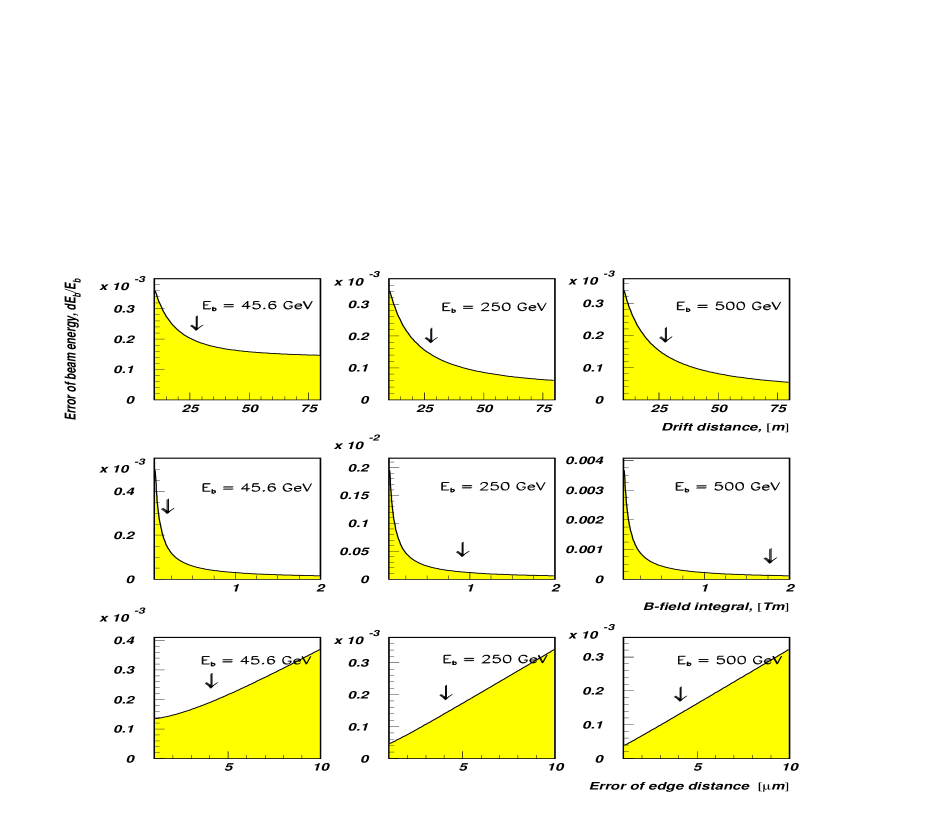
Figure 12: Beam energy uncertainty as a function of drift distance, B-field integral and edge displacement error for the $CO_{2}$ laser and three beam energies. The arrows in the histograms show the default values of the corresponding variable. For the variables not shown, the default values are used. The detector is placed 25 m downstream of the magnet.

In particular, at 45.6 GeV a stronger B-field would improve ${\Delta E_{b}}/{E_{b}}$ substantially, while at 250 and 500 GeV an improved edge displacement measurement or a larger drift space or some better knowledge of the B-field strength results to less significant improvements of $\Delta E_{b}/E_{b}$.

A peculiar problem which we have to account for is the amount of synchrotron radiation generated when the beam electrons pass through the dipole magnet and its possible impact on precise position measurements. This will be discussed in Sect.3.7.1.

3.3 Method B

Beam and Compton scattered electrons with energy $E$ propagate to the detector such that their transverse position is well approximated by

$$X(E)=X_{0}+\frac{A}{E}~{},$$ (22)

where $A\sim L\cdot\int Bdl$ and $X_{0}$ the position of the original beamline extrapolated to the detector plane, which is given by the center-of-gravity of the backscattered $\gamma$-rays, $X_{\gamma}$. Note that in (22) small effects related to synchrotron radiation are omitted.

According to eqs.(8) and (22), the positions of the beam and edge electrons can be expressed as

$$X_{beam}\equiv X(E_{beam})=X_{\gamma}+A/E_{beam}$$ (23)

$$X_{edge}\equiv X(E_{edge})=X_{beam}+A\cdot\frac{4\omega_{0}}{m^{2}}~{}.$$ (24)

Hence, the beam energy can be deduced from

$$E_{b}=\frac{m^{2}}{4\omega_{0}}\cdot\frac{X_{edge}-X_{beam}}{X_{beam}-X_{\gamma}}~{}.$$ (25)

Thus, instead of recording the energy of the edge electrons, the beam energy can be accessed from measurements of three particle positions, the position of the forward going backscattered $\gamma$-rays, the position of the edge electrons and the position of the beam particles. The position $X_{beam}$ can be measured by a beam position monitor (BPM), while recording $X_{edge}$ and $X_{\gamma}$ needs dedicated high spatial resolution detectors very similar to the demands of method A.

Besides the limitation to a $CO_{2}$ laser for the concept of edge energy measurements (method A), the demand of $2\cdot 10^{-5}$ for the field integral uncertainty is rather challenging, and less stringent requirements would be of great advantage. In method B, $E_{b}$ determination does not depend on the field integral, the length of the magnet as well as the distance to the detector plane. In particular, the independence on the integrated B-field only requires rather coarse $\Delta B/B$ monitoring. It is, however, necessary to ensure that both the beam and the edge electrons have to pass through the same B-field integral, i.e. the magnetic field has to be uniform across the large bending range. Also, the distance $X_{edge}-X_{beam}$ in (25) which involves as a product the integrated B-field and the sum of the drift distance and the length of the magnet [19], does not depend on the beam energy. Possible variations of this distance may only be caused by rather slow processes of environmental nature. Thereby, by accumulation of many bunch related $X_{edge}-X_{beam}$ measurements, high statistical precision can be achieved for this quantity. This implies the option to operate the spectrometer with lasers of less pulse power, which is of great advantage since the laser pulse power is a critical issue for method A. The novel approach of recording three particle positions (the three-point concept) seems therefore a very promising alternative.

Also, eq.(25) reveals that due to the proportionality between the beam energy and the distance $X_{edge}-X_{beam}$, which is larger as smaller the wavelength of the laser, best beam energy values are obtained for high energy lasers, a situation which is opposite to that of method A.

The precision of the beam energy can be estimated as

$$\frac{\Delta E_{b}}{E_{b}}=\frac{X_{edge}}{X_{edge}-X_{beam}}(\frac{\Delta X_{edge}}{X_{edge}})\oplus\frac{X_{edge}}{X_{edge}-X_{beam}}(\frac{\Delta X_{beam}}{X_{beam}})\oplus\frac{\Delta X_{\gamma}}{X_{beam}}~{}.$$ (26)

Here, the three terms have to be added in quadrature. Assuming for the crossing angle 10 mrad and (achievable) values for $\Delta X_{beam}$ = 1 $\mu$m and $\Delta X_{\gamma}$ = 1 $\mu$m, expected beam energy uncertainties are shown in Fig. 13 against the edge position error, $\Delta X_{edge}$, for the $CO_{2}$, infrared and green lasers at 250 GeV, in analogy to Fig. 11. Drift distances of 25 or 50 m and beam bend angles of 0.5 or 1 mrad are supposed. Clearly, for edge position errors of 10 $\mu$m and a limited drift range of 25 m,

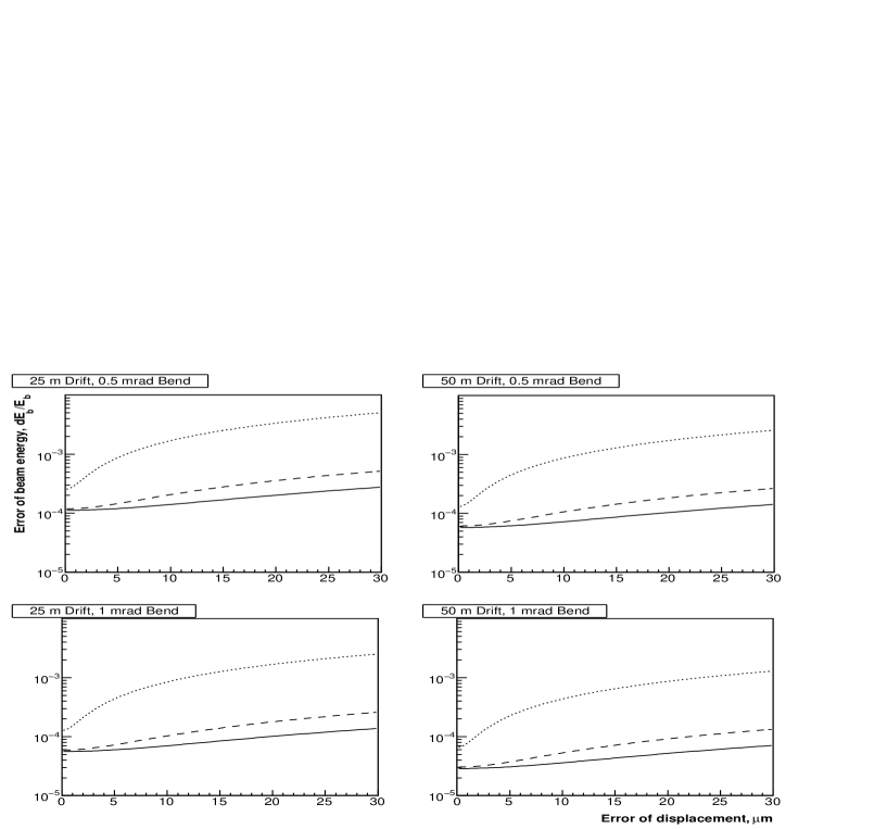
Figure 13: Beam energy uncertainty as a function of the edge position error for the green laser (full curve), the infrared laser (dashed curve) and the $CO_{2}$ laser (dotted curve) for $\Delta X_{beam}$ = $\Delta X_{\gamma}$ = 1 $\mu$m, two values of the drift space and bending angle. The beam energy is 250 GeV.

$\Delta E_{b}/E_{b}$ = 10^-4 can only be achieved by employing an infrared or a green laser. A $CO_{2}$ laser should not be considered as an option for this approach since $\Delta E_{b}/E_{b}$ exceeds very quickly the anticipated limit of $10^{-4}$ if $\Delta X_{edge}$ becomes few micrometers. Even for a perfect edge position measurement, i.e. for $\Delta X_{edge}$ = 0, the precision of the beam energy is often larger than $10^{-4}$.

In Fig. 14, $\Delta E_{b}/E_{b}$ values are plotted against the accuracies of the edge, beam and $\gamma$-ray positions for the infrared laser, a 25 m drift distance and a bend angle of 1 mrad for three beam energies. We also assume $\Delta X_{edge}$ = 8 $\mu$m, $\Delta X_{beam}$ = 1 $\mu$m and $\Delta X_{\gamma}$ = 1 $\mu$m as default values. Utilizing these values, $\Delta E_{b}/E_{b}$ results to 3.74 (0.91, 0.66) $\cdot 10^{-4}$ at 45.6 (250, 500) GeV in good agreement with the demands. Improvements for the $Z$-pole value are possible by employing e.g. a green laser and/or better $X_{beam}$ and $X_{\gamma}$ position measurements.

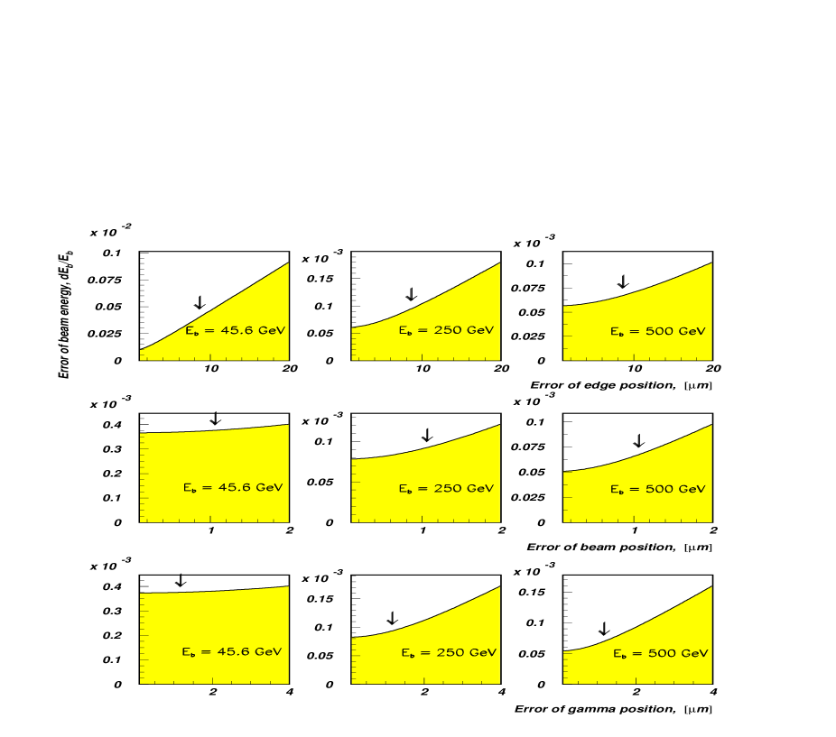
Figure 14: Beam energy uncertainty as a function of the errors of the edge, beam and Compton photon positions for the infrared (1.165 eV) laser and three beam energies. The arrows in the histograms show the default values of the corresponding variable. For the variables not shown, the default values are used. The detector is placed 25 m downstream of the magnet.

3.4 The Vacuum Chamber

In order to maximize the Compton signal, the location of the laser crossing point should be close to a waist of the electron beam. Having such a position found, the usual round electron beam pipe with typically 20 mm diameter will be replaced by a rectangular vacuum chamber with entrance and exit windows for the laser beam. Crossing of the two beams is assumed to occur at the center of the chamber. All particles generated at the IP should be conveniently accommodated by the chamber without wall interactions.

We plan vertical crossing of the laser light, utilizing a non-zero but small crossing angle of 8-10 mrad. Small crossing angles avoid $e\gamma$ luminosity loss. For lasers with short ($\simeq$10 ps) pulses, the degree of sensitivity of the luminosity to the relative timing of the two interacting beams and the laser pulse length itself is less critical. However, the benefits of a small crossing angle must be balanced against possible luminosity loss associated with an enlarged laser focus. A quantitative analysis must consider the wavelength dependent emittance of the laser, the pulse length and time jitter together with the geometry of the vacuum chamber and the laser beam optics ( see Sect.3.6 for some details).

The form and size of the vacuum chamber are mainly dictated by the trajectories of the unscattered beam, the Compton scattered particles and the laser properties. We propose to replace the original round beam pipe near the IP by a 6 m long vacuum chamber with rectangular cross section of $x\times y=60\times 60$ mm² in order to accommodate both beams conveniently. The laser beam will be, after passing through the entrance window, focused by a parabolic mirror with high reflectivity to the interaction region, as sketched in the top part of Fig. 15. The window might be a vacuum-sealed $ZnSe$ coated window

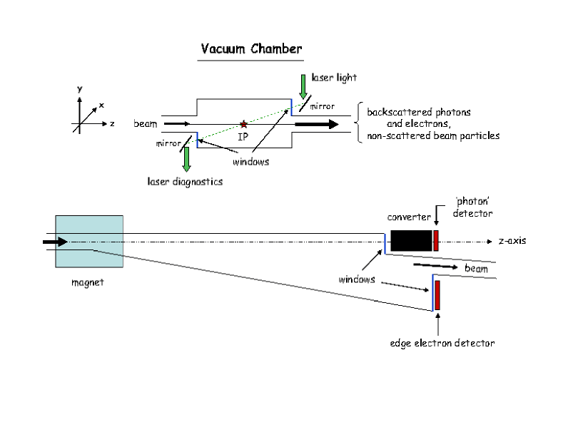
Figure 15: Top: side view of the laser beam crossing vacuum chamber. Bottom: top view of the vacuum chamber downstream of the magnet.

that introduces the laser light into the vacuum. It is mounted about 3 m off the IP nearly perpendicular to the beam direction with a vertical offset of 25 mm from the beamline. This geometry ensures almost head-on collision of the laser light with the incident electrons.

After passing through the IP, the laser beam leaves the chamber through the exit window. After some redirection by a second mirror, the laser light enters a powermeter for monitoring the power or a wavemeter to control the spectral position of the laser line. The chamber does not require internal vacuum mirrors since optical components installed in the vacuum are susceptible to be damaged by the beam or synchrotron radiation. For this reason it is proposed to mount the mirrors outside the vacuum at positions as indicated in Fig. 15.

Near the position of the entrance window the vertical dimension of the vacuum chamber is reduced to 20 mm, so that the cross section becomes 60$\times$20 mm². In this way, the entrance (and exit) mirror together with small mounts and adjustment devices can be placed close to the beamline. The rectangular shape of the chamber is continued up to the center of the magnet and increases from here continuously towards the deflection direction, as indicated in the bottom part of Fig. 15. The vertical chamber size of 20 mm will be kept up to the detector plane. Thus, particles with different deflection angles are well accommodated and tracked in ultra-high vacuum up to their recording by the detectors. Also, in order to minimize wake field effects, variations of transverse dimensions of the chamber should be smooth. For a fixed bending power of 1 mrad, the actual horizontal size of the chamber varies strongly with the laser wavelength. Tab. 1 collects the horizontal extensions of the chamber with respect to the incident beam direction, $x_{right}$ and $x_{left}$, for three laser and beam energies at the exit of the magnet and the detector plane located 50 m further downstream. A safety margin of 5 mm toward negative x-values has always been added. Note, a $CO_{2}$ laser needs smallest chamber sizes due to largest edge electron energies. Near the detector position, the vacuum chamber is largely modified and reduced to the usual round beam pipe with 20 mm diameter. Here, the BPM for beamline position measurements has to be incorporated. Large exit windows (of e.g. 0.5 mm Al) in front of the photon converter and edge detector allow the Compton scattered particles to leave the vacuum.

Beam energy,	Laser energy,	Edge energy,	x-values	x-values
GeV	eV	GeV	at magnet exit, mm	at detector plane, mm
45.6	0.117	42.15	10 / -7	10 / -32
	1.165	25.14	10 / -8	10 / -53
	2.330	17.35	10 / -9	10 / -75
250.0	0.117	172.6	10 / -7	10 / -43
	1.165	45.77	10 / -13	10 / -150
	2.330	25.19	10 / -20	10 / -268
500.0	0.117	263.70	10 / -8	10 / -55
	1.165	50.39	10 / -20	10 / -268
	2.330	26.53	10 / -33	10 / -505

Table 1: Extensions of the vacuum chamber in x with respect to the incident beam direction, $x_{right}$ and $x_{left}$, for three laser and beam energies at the exit of the magnet and the detector plane. A safety margin of 5 mm towards the bending direction has been added. The detector is assumed to be located 50 m downstream of the magnet.

3.5 The Magnet

In this note we propose, as a first step, to employ the magnet as discussed in Ref.[1]. The magnet has a wide gap of $170\times 35$ mm² to simultaneously accommodate all particle trajectories over a wide range in energy and magnetic field monitoring devices. The bend angle for beam electrons between 45 and 500 GeV, specified to be 1 mrad, results in a field integral of 0.84 T$\cdot$m at 250 GeV.

Estimation and optimization of the parameters for the magnet were performed by a series of 2D and 3D computer model calculations [23, 24, 25, 26, 27]. The proposed C-type solid iron core magnet has a length of 3 m. Mirror end plates are installed to contain the fringe fields. The magnet proposed facilitates vacuum chamber installation and maintenance as well as simplifies magnetic field measurements. The transverse cross section of the magnet is shown in Fig. 16 and its main characteristics are listed in Tab. 2.

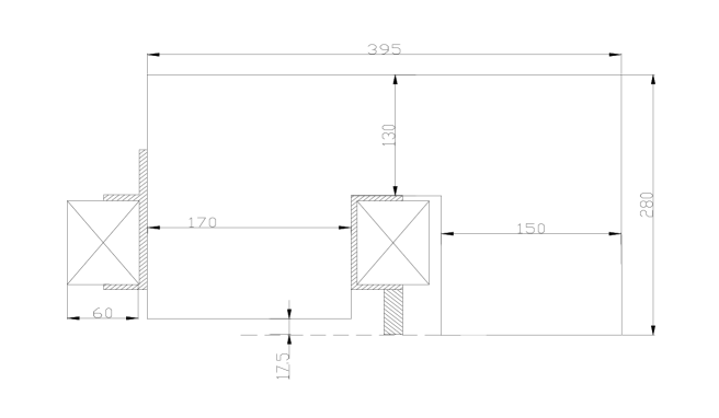
Figure 16: Cross section of the spectrometer magnet (1/2 part).

	spectrometer magnet
Magnetic field (min/max)(T)	0.05/0.55
Pole gap (mm)	35
Yoke type	C
Yoke dimensions (mm)	395x560x3000
Yoke weight (t)	4.51
A∗turns (1 coil)(max)	6335
Number of turns (1 coil)	6∗4=24
Conductor type, sizes (mm)	Cu, 12.5x12.5, ${\oslash}7.5$
Conductor weight (t)	0.36
Coil current (max)(A)	264
Current density (max)(A/mm2)	2.4
Coil voltage (max)(V)	13.3
Coils power dissipation (max)(kW)	3.5
Number of water cooling loops	6
Length of cooling loop (m)	56
Water input pressure (Bar)	6
Water input temperature (deg C)	30
Maximal temperature rise of the	1.4
cooling water (deg C)

Table 2: Basic technical parameters of the spectrometer magnet.

The magnet iron core is divided into only two parts by a horizontal symmetry plane. This decision gives confidence for tight tolerances of the parallelism of the magnet poles and would decrease substantially field distortions from the joining elements. The coils of the magnet are proposed to be made from 12.5 mm² copper conductors with water cooled channels of 7.5 mm diameter. Each pole coil consists of three double pancake coils (4 turns in two layers). According to 3D field simulations, a field integral uniformity of 20 ppm was found over almost 20 mm for the anticipated beam energies.

More details of the magnet are discussed in [1], which includes production tolerances, demands for the materials, fringe field limitations, temperature stabilization and cooling system, zero-field adjustment, power supplies and the control system. The overall objective of the field integral uncertainty of $2\cdot 10^{-5}$ might be achievable by accounting for all these aspects. If the field integral uniformity region is, due to manufacturing errors, somewhat reduced, a fraction of beam energy-laser energy combinations in Tab. 1 has to be reconsidered. Whether a redesign of the magnet is necessary depends on its final properties and the choice of the laser. If beam energy determinations will be performed by means of precise edge electron measurements (method A), the uniformity region with 20 ppm uncertainty has to be adjusted such that the path of the edge electrons is properly covered by the B-field.

The uncertainty of the field integral $\Delta B/B=2\cdot 10^{-5}$, a demanding request, needs careful design and production of the magnet, accurate field calibration and monitoring. Thorough mapping of the field in the laboratory under a variety of conditions that are expected during operation is essential and monitoring standards should be calibrated with sufficient accuracy. We propose two independent, high precision methods to measure the field integral as well as the field shape of the magnet: (i) the moving wire technique as e.g. described in [28] and (ii) the moving probe technique, where the field integral is obtained by driving NMR and Hall probes along the length of the magnet in small steps.

When the magnet is installed in the beamline, absolute laboratory measurements should be used to simultaneously calibrate three independent, transferable standards for monitoring the field strength: (i) a rotating flip coil, (ii) stationary NMR probes and (iii) a current transductor [28]. Since a $2\cdot 10^{-5}$ field integral precision is envisaged, performance of the magnet and the monitors, in particular the stability of the power supply current and the magnet temperature, have to be investigated.

In addition to the field of the spectrometer dipole itself, other sources of fields are expected in the ILC tunnel which might affect the path of the Compton electrons. The earth’s magnetic field, for example, should be measured and corrected for. Also fields produced due to currents to drive magnets in the beamline might be non-negligible and time-dependent. Therefore, the ambient field strength in the tunnel has to be explicitly monitored and corrections applied to avoid spurious bends on the Compton electrons while they travel to the detector.

The requests for the magnet are less demanding for the alternative method B where the positions of the Compton edge electrons and photons as well as of the beam particles are recorded.

3.6 The Optical Laser System

3.6.1 General Aspects

In order to achieve the necessary $e\gamma$ luminosity and rate of Compton events the laser system should provide pulse energies, duration and repetition rates as required. The initial parameters of the beam and its optical quality should drive the design of an adequate laser transport system. The basic scheme of the laser source contains a master oscillator which provides the initial laser pulse pattern that matches that of the incident electron bunches. Additional amplification might be needed to achieve the necessary pulse energy.

Propagation of laser light is usually considered in the framework of the Gaussian beam optics, and by definition, the transverse intensity profile of a Gaussian beam with power $P$ can be described as [29]

$$I(r,s)=\displaystyle\frac{P}{\pi w(s)^{2}/2}\exp\Biggl{\{}-2\displaystyle\frac{r^{2}}{w(s)^{2}}\Biggr{\}}\;,$$ (27)

where the beam radius $w(s)$ is the distance from the beam axis to the $1/e^{2}$-intensity drop, and $s$ denotes the coordinate along beam propagation. It is important to note that this definition of the beam radius is twice as large as the usual Gaussian ’sigma’, $w(s)=2\cdot\sigma(s)$. In practice, the transverse intensity profile of lasers, operating in the TEM₀₀ mode, is only close to but not exactly a Gaussian. A pure Gaussian beam has as lowest possible beam parameter product the quantity $\lambda/\pi$ (with $\lambda$ the laser wavelength), whereas for real beams the beam parameter product is defined as the product of the beam radius (measured at the beam waist) and the beam divergence half-angle (measured in the far field). The ratio of the real beam parameter product to the ideal one is called $M^{2}$, the beam quality factor.

In free space, the beam radius varies along the traveling direction according to

$$w(s)=w_{0}\cdot\sqrt{1+\Biggl{(}\displaystyle\frac{M^{2}\lambda s}{\pi w_{0}^{2}}\Biggr{)}^{2}}\;,$$ (28)

with $w_{0}=w(s=0)$ as the beam radius at the waist. The radius of curvature $R$ of the wavefronts evolves as

$$R(s)=s\cdot\Biggl{[}1+\Biggl{(}\displaystyle\frac{\pi w_{0}^{2}}{M^{2}\lambda s}\Biggr{)}^{2}\Biggr{]}\;$$ (29)

and the beam status at a certain position $s$ can be specified by a complex parameter $q$:

$$\frac{1}{q(s)}=\displaystyle\frac{1}{R(s)}+\displaystyle\frac{iM^{2}\lambda}{\pi w(s)^{2}}\;.$$ (30)

The passage of the beam through optical elements may be characterized by transforming $q$ utilizing an $ABCD$ matrix for each element [29, 30]:

$$q^{\prime}=\displaystyle\frac{Aq+B}{Cq+D}\;,$$ (31)

and by multiplying all matrices the whole system is described.

3.6.2 Final Focus Scheme

For largest $e\gamma$ luminosity, the laser beam delivery system should provide the lowest possible waist size at the crossing point. But due to alignment uncertainties and possible relative laser and electron beam position jitters, options to adopt best waist sizes have to be foreseen. This requirement can easily be achieved when a short-focus lens doublet is used for the final focusing system close to the interaction area. Fig. 17 shows for a particular laser optics and a crossing angle of 10 mrad, irrespective of the laser wavelength, the 1$\sigma$ beam size of the laser near the crossing region.

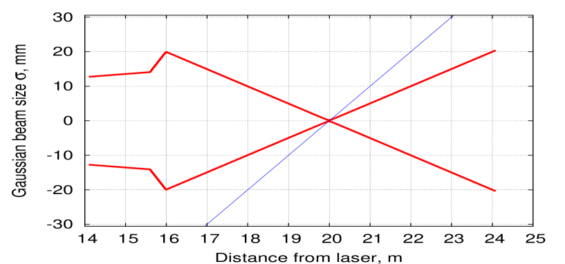
Figure 17: 1$\sigma$ laser beam size near the crossing region with $\alpha$ = 10 mrad. The thick line represents the laser beam, while the thin line shows the incident electron trajectory.

The waist is positioned 20 m away from the laser exit aperture. The beam is focused by two lenses, $L_{1}$ and $L_{2}$, with focal length $f_{1}$ =-1.0 m, respectively, $f_{2}$ = 1.0 m. In order to avoid an additional waist between the two lenses, the first focal length has to be negative. The lenses are positioned at 15.600 m and 15.992 m, see Fig. 17, where the laser beam enters the vacuum chamber 17 m downstream from the laser exit aperture, and 3 m prior to the interaction point. The position of one of the lenses is supposed to be accurately adjustable by precise mechanics. The thin line in Fig. 17 indicates the corresponding electron beam line. Since the optical system was designed for a crossing angle of 10 mrad, limits are imposed on the laser beam divergence, $LD$, after the final focus system. The divergence (at 1$\sigma$ transverse laser beam size) has to be at least two times smaller than $\alpha$. Thus, for strict Gaussian beams, the acceptance of the beam delivery system should be larger than $2\sigma$, which is the reason for the assumed laser angular divergence of 5 mrad in Fig. 17.

The laser waist size is coupled to the laser beam angular divergence via

$$\sigma_{waist}=\frac{M^{2}\lambda}{4\pi LD}~{},$$ (32)

which is derived from (28). Minimal possible waist sizes and $M^{2}$ values so obtained are summarized in Tab. 3. $M^{2}$ varies with $E_{\lambda}$ according to typical parameters of the laser sources. The assumed laser spot sizes at the crossing point of 200, 100 and 50 $\mu$m for the $CO_{2}$, respectively, infrared and green laser are in accord with the numbers given in Tab. 3.

Laser	$E_{\lambda}$	$M^{2}$	$\sigma_{waist}$ ($LD=\alpha/2$)	$\sigma_{waist}$ ($LD=\alpha/3$)
$CO_{2}$	0.117 eV	1.1	186 $\mu$m	280 $\mu$m
$Nd:YAG$	1.165 eV	1.2	20 $\mu$m	30 $\mu$m
$Nd:YAG$	2.330 eV	1.3	11 $\mu$m	17 $\mu$m

Table 3: Possible minimal laser waist sizes and $M^{2}$ values for different laser energies and a crossing angle of 10 mrad.

Since the beam and the laser widths are of similar size, central collisions of both beams is essential in order to avoid systematic shifts of the center-of-gravity of the Compton photons. To ensure such collisions we propose to install a partially transmitting mirror close to the vacuum entrance window so that most of the laser light is employed for Compton collisions and only a small fraction hits a CCD camera or an avalanche photodiode (APD). The camera, respectively, the APD is used in the alignment procedure to permanently steer the laser onto the electron beam. Spot size and position of the laser can so be monitored. A feedback system allows to adjust the focus by the last mirror in the laser beamline, which might be a deformable or segmentable one. Smallest displacement of both beams from one another can be maintained by performing a scan that samples across successive electron bunches for highest Compton event rate. The required laser pointing stability should be $\sim$10 $\mu$m which seems to be achievable [31]. Furthermore, upstream and downstream of the collision chamber beam position monitors may be needed to monitor the position of the electron beam. More discussions about requirements for central collisions can be found in Sect.3.11.

3.7 Electron and Photon Detection

The detector assembly is supposed to be located at least 25 m downstream of the magnet. Since we plan to operate the spectrometer with an energy independent fixed bending angle of 1 mrad, the distance of the backscattered $\gamma$-ray centroid to the beamline 25 m downstream of the dipole is 26 mm for all $E_{b}$ values, while the displacement of the edge electrons depends on $E_{b}$ and $E_{\lambda}$. This displacement in the range of a few centimeters to about a quarter of a meter requires high stability of the detector assembly and its adjustment to micrometer accuracy. Therefore, the individual detector components should be connected rigidly and installed on a vibration damped table that can be moved horizontally (and vertically) and controlled with high precision.

After leaving the vacuum chamber, the Compton scattered electrons near the edge traverse a position sensitive detector with high spatial resolution. We propose to employ either a diamond micro-strip or an optical quartz fiber detector. Such detectors, frequently applied in particle physics experiments, have demonstrated their ability to achieve micrometer spatial resolution within an intense radiation field, see e.g. [32, 33].

The center-of-gravity of the Compton $\gamma$-rays might be recorded by employing one of the two following concepts. One concept consists in measuring high energy electrons and positrons from photon interactions in a converter placed closely in front of the tracking device. According to simulations, a tungsten converter of sufficient radiation lengths seems to be suitable. Such a scheme, however, constitutes some trade-off between large conversion rates and accurate photon position determinations, which might be altered by multiple scattering of the forward collimated $e^{\pm}$ particles within the converter. As a position sensitive detector a quartz fiber detector similar to that for edge position measurements is proposed and, as simulation studies revealed, submicrometer precisions of the original photon position are achievable.

An alternative for measuring $X_{\gamma}$, respectively, the undeflected beam position consists in monitoring one of the edges of the synchrotron radiation (SR) generated in the dipole magnet of the spectrometer. A detector sensitive to SR and ’blind’ with respect to high energy Compton photons would be appropriate for this task. For this option, a converter is not needed and all $\gamma$-rays are incident on the edge position detector.

3.7.1 Synchrotron Radiation

Synchrotron radiation will be generated by electrons passing through the magnet. For the magnet as described in Sect.3.5, about five photons per beam particle with an average energy of 3.8 MeV are generated, resulting to a total number of $10^{11}$ $\gamma$’s per bunch. They are concentrated within the cone of the forward produced Compton scattered photons and the bent beam. If a tungsten converter of e.g. 16 radiation lengths ($X_{0}$) in front of the $X_{\gamma}$ detector is inserted, it also serves as an effective shield against SR. However, the huge amount of such photons (plus a minor fraction from Compton scattered electrons) may preclude perfect SR protection. Possible low energy electrons and positrons from SR showers are expected to enter the detector and could modify the response and eventually the center-of-gravity of the primary Compton photons. The impact of this background (together with machine related background) has to be taken into account in procedures of precise $X_{\gamma}$ determinations. Properties of particles leaving the converter and prescriptions addressed to eliminate center-of-gravity distortions are discussed in Sect.3.8. Discussions on whether recording the incident beam position by means of SR is superior to the conventional converter approach are also included in this section.

3.7.2 Diamond Strip Detectors

A potential candidate for the high spatial resolution tracking device is the diamond strip detector (DSD). Chemical vapor deposition strip detectors indicate, due to their inherent properties, that they are very radiation resistant. They are a promising, radiation hard alternative to silicon detectors. In addition, diamond is favored over silicon due to its smaller dielectric constant, which yields a smaller detector capacity and, thereby a better noise performance. It is also an excellent thermal conductor with thermal conductivity exceeding e.g. that of copper by a factor of five.

When a minimum ionizing particle traverses the diamond, 36 electron-hole pairs are created per micrometer due to Coulomb interaction, Bremsstrahlung and scattering with electrons along its path. Per electron-hole pair, a mean energy deposit of 13 eV is needed. The electric field in the volume causes a drift of the electrons and holes across the diamond to the positive, respectively, negative electrode. The induced current produces a signal, which can be amplified and integrated resulting in a voltage signal proportional to the total charge.

The spatial resolution of DSD’s is obtained by segmentation of the anode (p⁺) into so-called micro-stripes. The micro-stripes might only be ten micrometer apart and this pitch determines the detector resolution. Employing the charge division method, the spatial resolution for single-particle passage can be further improved compared to the binary resolution of $pitch/\sqrt{12}$. In this way, the resolution of large scale diamond strip detectors with a pitch of e.g. 50 $\mu$m was found to be in the range of 7-15 $\mu$m [34, 35, 36, 37] which is better or close to the binary resolution of 14.4 $\mu$m. Also, excellent linearity of the detector system over four decades of incident particles was observed [34].

Diamond strip detectors were also used as beam monitors [38, 34, 36] to access the cross-sectional beam profile online for single bunches. In particular, Ref.[38] proposed to perform such measurements for the TESLA linear collider with $2\cdot 10^{10}$ electrons per bunch. Tests in heavy ion and electron beams with up to $3\cdot 10^{10}$ particles/bunch were successfully performed although the precision of the measurement was difficult to estimate. In our approach, the number of instantaneous particles incident per readout pitch is at most few hundred for endpoint position (or thousands for $X_{\gamma}$) measurements and hence orders of magnitude smaller than for bunch profile measurements. The spatial resolution in cases of high occupancy is, however, expected to be slightly worse than for single-particle crossing mainly due to $\delta$-electrons and spreading of charge carriers inside the active volume of the detector, especially if the electric field inside the sensor breaks down. For example, a resolution of 23 $\mu$m was measured for a 50 $\mu$m pitch detector [35]. Reduction of the thickness of the sensor to e.g. 80 $\mu$m and shorter strips should improve the resolution.

The main parameters of a DSD are the thickness which the ionizing particles cross, the strip pitch and its width. The typical bias depletion voltage is 1 V/$\mu$m. More details of such a device will be discussed in Sect.3.8.

3.7.3 Quartz Fiber Detectors

In view of the properties of a detector for precise edge position and $\gamma$-ray centroid measurements a suitable option consists in a detector of quartz fibers. This option is driven by several aspects such as high spatial resolution, fast signal collection such that all charges associated with one bunch crossing are collected before the next bunch crossing, very high radiation hardness and the insensitivity to induced activation and possible consequences on measurements. In addition, tracking detectors based on quartz fibers (QFD’s) are simple in construction and operation. They do not need any internal calibration and can work at very high flux. The availability of square fibers today allows to construct a detector of e.g. 100 or even 50 $\mu$m fibers with excellent spatial resolution.

In quartz, the signals are caused by Cerenkov light production for which quartz is transparent, predominantly for ultraviolet light within the 300 to 400 nm wavelength region. Cerenkov radiation is intrinsically a very fast process with a typical time constant of less than 1 ns. Instrumental effects (e.g. those caused by light detection devices) may broaden the signal, but still the overall charge collection time is less than 10-20 ns. The fibers are readout by photodetectors which are usually placed as close as possible to the sensitive layer.

The so-called lightguide condition in optical fibers together with the fact that Cerenkov light emitted inside the fiber has a specific angle with respect to the particle direction leads to an angle dependent light output at which the particles traverse the fiber. The production of Cerenkov light is maximum for particles passing the quartz fiber axis at angles of incidence of 40⁰-50⁰ .

A potential drawback of a quartz fiber detector constitutes to the low light yield for single-particles. One expects typically 1-3 photoelectrons/GeV incident energy [p.e./GeV], but yields of 10 p.e./GeV were reported [33]. We expect, however, due to the large number of Compton scattered particles per fiber no limitations of photoelectron statistics compared to other sources of fluctuations.

Many of quartz fiber detectors are calorimeters, see e.g. [39]. Quartz fibers were chosen as active material, with diameters ranging from $\sim$800 to 270 $\mu$m, and often both the energy and impact position of particles are measured. Spatial resolutions of typically a fraction of a millimeter were achieved. Other applications consist in beam diagnostics systems in harsh radiation environments [40] and in tracking and vertexing in HEP experiments [41]. Recently, the ATLAS collaboration [42] proposed a fiber tracker for luminosity measurements with a spatial resolution of approximately 15 $\mu$m. However, fiber trackers for precise particle profile measurements as anticipated in this study were, to our knowledge, not employed.

Our baseline configuration of a quartz fiber detector utilizes square fibers with a size of 50 $\mu$m having the advantage that their effective thickness is roughly the same for all traversing particles. Due to the small fiber length of few centimeters geometrical constraints for precise micrometer measurements are of no concern. A cladding thickness of 5 $\mu$m results in an active fiber core of 40 $\mu$m. Despite of the high occupancy sufficient position resolution is expected, in particular for a staggered layer arrangement. Since in our case practically all electrons pass the detector with $90^{0}$ angle of incidence, little light emission is expected. Therefore, we propose to incline the detector by $45^{0}$ with respect to the vertical direction so that large signals are obtained which can be conveniently extracted and transported to the shielded location for the readout electronics. Fiber ends are coupled through an air lightguide to a photomultiplier tube (PMT). Whether it is worthwhile to polish the opposite end of the fibers to enhance the light reflection needs further studies. Typical solutions for QFD readout use PMT’s with multi-anode structure. Such PMT’s are well established and robust, and crosstalk between channels is at the level of only 2-3%.

For both the DSD and QFD detector schemes the sensitive region of the device can be small, in the order of $1\times 1$ cm², since only the position of electrons at or close to the edge, respectively, the center-of-gravity of the forward produced Compton photons is of interest. Thereby, a relative small number of readout channels is needed, and, together with some fast and robust data processing, the system should provide position information of micrometer resolution. It is advantageous to house the detector assembly inside a Roman Pot. In the case of a quartz fiber detector, $\mu$-metal shielding for PMT’s is required in the presence of stray magnetic fields in excess of 10 Gauss in order to maintain the gain and hence the detection efficiency. The output signal can be readout by a relatively simple binary electronics chain, for which an example is given in [42]. Even for a relative small single fiber detection efficiency of 70 to 80%, excellent overall performance of the detector is expected.

3.7.4 Photon Detector Options

One possibility to perform $X_{\gamma}$ measurements consists in using a quartz fiber detector in conjunction with a closely placed converter of adequately chosen radiation length. Compton backscattered photons will be affected during their propagation through the converter by several processes such as ($e^{+},e^{-}$)-pair creation and Compton collisions. Once $e^{\pm}$ particles are created, they are subject to multiple scattering, ionization, and $\delta$-ray production, bremsstrahlung and annihilation of positrons. After some tracking, the particles either stop, interact or escape the converter. The converter, e.g. tungsten of 16 $X_{0}$, primarily aims to convert the high energy Compton $\gamma$-rays to $e^{\pm}$ particles, since only charged particles generate Cerenkov light within quartz fibers. The position of the strongly forward collimated photons is maintained by the $e^{\pm}$ shower profile when escaping the converter, as demonstrated by simulation in the next section. SR photons constitute some background and, due to their asymmetry with respect to x = 0, they can disturb the original position of the Compton photons after pair creation. Therefore, the converter should absorb most of these photons and $X_{\gamma}$ position measurements have to account for some possible residual asymmetric detector response. The converter is supposed to have a cross section of $2\times 2$ cm² and a length of 16 $X_{0}$. The transverse dimension of the converter is mainly dictated by the small displacement of the beam particles 25 m downstream of the spectrometer magnet. A converter of e.g. 26 $X_{0}$ with more efficient SR removal results to less precise $\gamma$-centroid measurements and is considered to be less favored.

A completely different way to record the undeflected beam position relies on monitoring the edge of SR light at x = 0, without a converter in front of the position device. Dedicated and novel SR devices were suggested in [43]. In this paper, we propose to employ the plane-parallel avalanche detector with gas amplification. SR light which passes a $10\times 10$ mm² entrance window of 1 mm beryllium generates an avalanche in xenon gas at 60 atm over a range of 1.5 mm, the gap between the anode and cathode. The transverse size of the avalanche is expected to be close or below 1 $\mu$m, and due to the amplification process, a large number of electrons is produced and generates a sufficiently strong output signal [43]. The anode plane of the detector consists of 1 $\mu$m nickel layers with 2 $\mu$m NiO dielectric separation in between. Such a geometry matches very well the transverse size of the avalanche and permits submicrometer access of the position of the SR edge. Since no converter is planed in this scheme, the $10^{6}$ high energy Compton photons are now background. Their impact on the accuracy of the SR edge is negligible as will be shown below.

3.8 Simulation Studies

A full Monte Carlo simulation based on the GEANT toolkit[45] has been developed to analyze the basic properties of the Compton spectrometer and to evaluate design parameters for the detectors. Bunches of $2\cdot 10^{10}$ electrons are colliding with unpolarized or circular polarized infrared or green laser pulses of 10 ps duration by a Compton generator. The generator accounts for an internal electron bunch energy spread of 0.15% which is slightly larger than the values given in [44] , a transverse bunch profile of 20 $\mu$m and 2 $\mu$m in horizontal, respectively, vertical direction and a 300 $\mu$m extension along the beam direction, all of Gaussian shape. An angular spread of 1 and 0.5 $\mu$rad in x-, respectively, y-direction has been assumed. Such input parameters are in accord with ILC beam properties within the BDS. A high-power pulsed laser with either $E_{\lambda}$ = 1.165 eV or 2.33 eV is focused onto the incident beam with a crossing angle of 8 mrad. The transverse spot size of the laser at the Compton IP is set to 100 (50) $\mu$m for the infrared (green) laser, and the laser angular spread was assigned to 2.50 (1.25) mrad. Also, perfect laser pointing stability and instantaneous laser power are assumed. As default event rate, $10^{6}$ Compton scatters are generated for single bunch crossing.

Compton recoil electrons and photons as well as non-interacting beam particles are tracked through the spectrometer and recorded by the detectors. A special vacuum chamber as sketched in Fig. 15 ensures negligible Coulomb scattering. The magnet provides a fixed bend of 1 mrad for all beam energies anticipated. At the nominal energy of 250 GeV, the magnet rigidity corresponds to 0.84 Tm for a magnet length of 3 m. The simulation also includes a 1% integrated B-field fraction for the fringe field. Synchrotron radiation with properties as discussed in [43] is enabled when electrons pass through the magnet. On average, a beam particle radiates about 5 photons with an average energy of 3.8 MeV and an energy spectrum that peaks below 1 MeV.

The position sensitive detectors which perform $X_{\gamma},X_{beam}$ and $X_{edge}$ measurements are located 25 m downstream of the spectrometer magnet. For the edge electrons, we assume either a diamond strip or a quartz fiber detector. Both detector options have a transverse size of $1\times 1$ cm². For the 100 $\mu$m thick diamond detector a pitch of 50 $\mu$m and a strip width of 15 $\mu$m were chosen. A crosstalk of 2% and a 99% detection efficiency were assumed. When passing through a thin layer of matter, charged particles lose energy which follows in good approximation a Landau distribution. Thereby, in rare cases the electron transfers a large amount of energy within the sensor which implies a large charge signal. A code based on GEANT has been written that simulates all physical processes taking place in the DSD and calculates the energy deposited along the particle track in the detector. The resulting deposited energy is used to weight each electron and, after summation over all entries in a given channel, the total signal is shown in the corresponding figures.

For the quartz fiber detector, Compton electrons are measured by a single layer of 50 $\mu$m square fibers. A cladding thickness of 5 $\mu$m on each side results in an active fiber core of 40 $\mu$m. Crosstalk between fibers was set to 3%. Largest response of the detector is obtained when the angle of particle incidence corresponds to the Cerenkov angle of 46^o. Therefore, the quartz fiber detector was inclined by 45^o with respect to the vertical direction. Since only a fraction of typically a few percent of the light produced in the fibers is trapped and transported to the light detector, the small probability to detect a minimum ionizing particle is to great extent compensated by the large number of electrons traversing a single fiber. Therefore, despite a small single-particle light yield, a detection efficiency for individual fibers of 95% was assumed. The quartz fiber response was simulated by counting the number of light photons generated by each electron along its path through the detector. The sum over all such photons within a fiber is proportional to the output signal and is plotted in the figures.

The profile of scattered electrons measured by both detectors considered is shown in Fig. 18. For an incident beam energy of 250 GeV, Figs. 18 (a) and (b) plot examples of simulated edge spectra for the diamond strip and quartz fiber detectors utilizing the 1.165 eV infrared laser. For the green laser with $E_{\lambda}$ = 2.33 eV, analogous spectra are displayed in parts (c) and (d) of the figure. All spectra are normalized to $10^{6}$ primary Compton events assumed for single bunch crossing. As can be seen, the expected sharp edges of the spectra are somewhat diluted, mainly due to the energy spread of the beam particles, angular dispersions, beam spot size, detector position resolution and crosstalk. The edge positions of the spectra were obtained by a fit of a function which results from a step-function plus a (uniform) background folded by a Gaussian as proposed in e.g. [6, 7]:

$$G(x,p_{1...6}) = \frac{1}{2}(p_{3}+p_{4}(x-p_{1}))\cdot\mbox{erfc}\left[\frac{x-p_{1}}{\sqrt{2}p_{2}}\right]$$ (33)

$$-\frac{p_{2}p_{4}}{\sqrt{2\pi}}\cdot\mbox{exp}\left[\frac{(x-p_{1})^{2}}{2p_{2}^{2}}\right]+p_{5}+p_{6}(x-p_{1})~{}.$$

The edge position $p_{1}$, the edge width $p_{2}$, the amplitude of the edge $p_{3}$, the slope $p_{4}$, the background level $p_{5}$ and its slope $p_{6}$ were treated as free parameters. Assuming $p_{5}$ = $p_{6}$ = 0 in our particular case, the errors of the edge positions were found in the range of 5 to 15 $\mu$m,

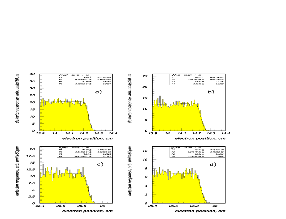
Figure 18: Infrared laser electron edge position simulations for a) a diamond strip detector and b) a quartz fiber detector. For the green laser the corresponding spectra are shown in c) and d). The incident beam energy is 250 GeV and the number of events were normalized to $10^{6}$ primary Compton scatters. The lines represent the result of the fits.

with values of 5 and 9 (12 and 15) $\mu$m for the infrared (green) laser. These numbers are in accord with the endpoint position demands shown in e.g. Figs. 13 and 14 for the approach of recording three particle positions, $X_{\gamma}$, $X_{beam}$ and $X_{edge}$. Similar uncertainties were obtained if 100 $\mu$m fibers with 10 $\mu$m cladding were utilized. It is also evident that method A based on direct edge energy measurements (by means of precise B-field integral and edge displacement information) seems to be nonfavored: precisions of edge electron displacements of a fraction of a micrometer up to only few micrometers (see Fig. 11) are difficult to achieve without additional effort.

In principle, the beam polarization may affect the endpoint $p_{1}$ which might be coupled with the slope of the energy spectrum $p_{4}$ in the vicinity of the edge position as indicated in Fig. 4. By Compton simulation of 80% polarized electrons of 250 GeV with circular polarized infrared laser light we found that the edge position differs by less than 1 $\mu$m with respect to the case of unpolarized electrons. Thereby, Compton scattering of polarized beams will not noticeably modify $p_{1}$ and hence the beam energy measurement.

The assumption of a Gaussian internal energy spread relies on ongoing machine design studies. As long as collective effects as intra beam scattering (IBS) or interactions with the vacuum chamber impedance are negligible the energy spread is expected to be of Gaussian shape. Since at present a final design of the vacuum chamber to minimize the beam impedance and IBS effects is not completed a realistic shape of the energy distribution is missing. Deviations from a Gaussian, if any, are however expected to be small [46]. Preliminary accelerator simulations reveal that the energy spread is close to a Gaussian distribution [47] and support our assumption. This holds for the electrons as well as the positrons despite different sizes of the relative energy spread. If it will be demonstrated by measurements that the energy spread is not Gaussian distributed, the fitting function (33) has to be modified according to the findings.

For the diamond detector, the number of electrons per 50 $\mu$m detector pitch is about 200 (110) for the infrared (green) laser. The deposited energy amounts to $4.0(1.6)\cdot 10^{-5}$ W, of which 90% is due to the current induced in the diamond and 10% due to ionization. The associated heat load is expected to be of no concern since the thermal conductivity of diamond is very high. The heat, locally induced, can propagate very quickly away before the next bunch arrives.

Using the density of diamond (3.5 g/cm³), the deposited energy as given above, a bunch crossing rate of $15\cdot 10^{3}$ Hz and $10^{7}$ seconds for a year of data taking, a radiation dose of 1.3 (0.5) MGy (with an uncertainty of about 30%) is expected. This level is considerably below irradiation level investigations by the RD42 collaboration [32] ensuring survivability of the detector.

For the quartz fiber detector, about 120 (70) scattered electrons cross a single fiber. Most of the energy loss of the electrons is caused by ionization, while emission of Cerenkov light constitutes only a minor contribution. The released energy within 70 $\mu$m fiber pathlength is approximately $2.6(0.8)\cdot 10^{-6}$ W, which together with the density of quartz ($SiO_{2}$) of 2.2 g/cm³ yields a radiation dose of 0.054 (0.021) MGy per year. Again, these levels are associated with an uncertainty of 30%. Since absorbed doses up to few hundred MGy were measured in quartz fibers without serious degradation [48], radiation damage of a quartz fiber detector for edge electron measurements will not matter at all.

Within the approach of measuring $X_{\gamma}$, the center-of-gravity of the Compton scattered $\gamma$-rays is measured indirectly via conversion to electrons and positrons within a 16 radiation lengths tungsten converter. When entering the converter, the photons are concentrated within a spot of approximately 250 $\mu$m r.m.s., a size which is dominated by the $\sim$1/$\gamma$ angular distribution of the Compton process. After a first estimate of the thickness of the converter, a full simulation of the 56 mm long conversion material has been performed. In particular, the process of converting the $10^{6}$ Compton photons together with the SR photons along with the trajectories of the resulting electrons and positrons through the converter and into the fiber detector was simulated. Despite the small transverse extension of the converter, the core of the shower particles caused by Compton photons is assumed to maintain the initial $\gamma$-centroid position (being at x = 0.0 in the simulation). Directly after the converter the quartz fiber detector array of 50 $\mu$m fibers has been placed in order to measure the $e^{\pm}$ shower particles from which the $\gamma$-centroid position has to be deduced. Fig. 19(left) shows the number of charged particles escaping the converter as a function of x, while their energy behavior is shown on the right-hand side. The spectra indicated as ’Signal’ are $e^{\pm}$ particles from Compton photons, whereas those marked as ’Background’ are from synchrotron radiation. We expect $1.5\cdot 10^{8}$ charged particles from $10^{6}$ Compton events, with an average energy of 25.8 MeV. Their density distribution, $dN/dx$, clearly peaks at x = 0.

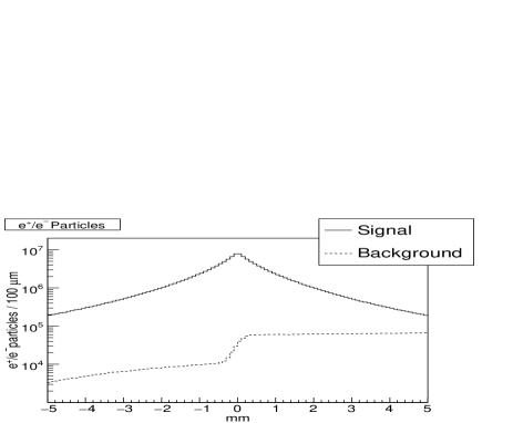
Figure 19: Left: Number of charged particles escaping the 16 radiation lengths tungsten converter as a function of x. Right: Energy distribution of charged particles escaping the converter. The ’signal’ spectra are normalized to $10^{6}$ Compton scatters, while the ’background’ spectra are normalized to $2\cdot 10^{10}$ beam particles within a bunch.

Besides of charged particles, photons also escape the converter. They are either generated within electromagnetic showers from Compton scattered and SR $\gamma$-rays or are SR photons which pass the converter without interaction. A fraction of less than 2% of the original SR yield with an average energy of 3.9 MeV survives. Their $dN/dx$ and energy spectra are shown in Fig. 20.

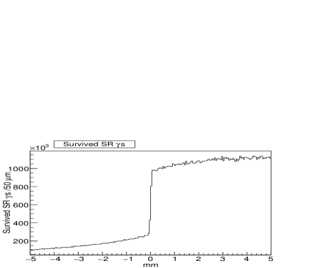
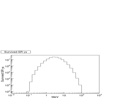
Figure 20: Left: Number of SR $\gamma$-rays which escape the 16 radiation lengths tungsten converter as a function of x. Right: Energy distribution of SR $\gamma$-rays escaping the converter. Both spectra are normalized to $2\cdot 10^{10}$ beam particles within a bunch.

The overwhelming fraction of the SR photons is converted to $e^{\pm}$ pairs and some of them ($3.5\cdot 10^{6}$) escapes the converter, see Fig. 19. They are expected to affect the $\gamma$-centroid position and have to be accounted for in any $X_{\gamma}$ determinations.

For the position sensitive $X_{\gamma}$ device, a single layer of quartz fibers is supposed with properties identical to those for the edge electron detector. Basically, this detector should have a large sensitivity to charged particles from pair production of Compton photons within the converter and ’blind’ with respect to background (SR) $\gamma$-rays. In Fig. 21, the response function of the detector in terms of the amount of Cerenkov light generated from all $e^{\pm}$ particles within a fiber is shown together with the result of a fit. An electron energy detection threshold of 0.6 MeV for Cerenkov light production is included. The fit result is based on a two-step procedure. First, due to an a priori unknown precise $\gamma$-centroid position, $X_{\gamma}$ is approximately determined by a simple algorithm [49], which fixes the peak position within about $\pm$25 $\mu$m. Then, selecting a fitting range of some $\pm$600 $\mu$m around this preliminary centroid, an empirical fit of the sum of three Gaussians and the step function in eq.(33), with $p_{4}$ = $p_{6}$ = 0, provides the ultimate peak position of $X_{\gamma}$ = -0.47 $\pm$0.54 $\mu$m with a $\chi^{2}/NDF$ = 16.59/14, corresponding to 27.8% probability.

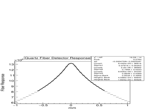
Figure 21: Cerenkov light response of all charged particles passing the quartz fiber detector. The curve is the result of a fit of the sum of three Gaussian distributions and the step function in eq.(33) with $p_{4}$ = $p_{6}$ = 0.

The fit range chosen excludes particles which are less sensitive to the peak position but sensitive to the background. The peak value found is in good agreement with the expectation of zero and its error is less than the anticipated limit of $\sim$1 $\mu$m. The spectrum in Fig. 21 resembles the response of all escaping $e^{\pm}$ particles generated from $10^{6}$ Compton photons and the appropriate fraction of SR, after normalization to $2\cdot 10^{10}$ beam electrons. The latter causes a slight asymmetry with respect to x = 0 and is the reason to include the step function within the fit. As a consequence, a rather complicated response behavior is obtained and after some trials the spectrum was reasonably described by the selected ansatz. If instead of a 50 $\mu$m fine segmented detector an array of 100 $\mu$m quartz fibers is utilized the centroid position and its error are found to be in agreement with the values quoted above. Irrespectively of the details for the final design of the converter-fiber detector system, this option seems to be capable to meet the requirements, in particular if instead of only one fiber layer several layers with some staggering are employed.

Basically, a different approach to record the incident beam direction consists of using a SR edge detector. The avalanche detector of Ref.[43] with xenon being in a superfluid state with a density of 3.05 g/cm³ is proposed to perform SR edge position measurements around x = 0. A detector acceptance of $\pm$5 mm will be exposed by some 20% of the $10^{11}$ SR photons and all $10^{6}$ Compton recoil $\gamma$-rays, which are considered now as background. Photons traversing the detector interact with the xenon so that electrons are created via e.g. the photoelectric effect or pair production. These electrons drift towards the anode and in collisions with xenon atoms they liberate further electrons. This process is accompanied by loss of energy of the electrons and deflection from their incident direction. The response of such a detector was simulated and the x-position of each electron-atom collision weighted by the corresponding released energy is plotted in Fig. 22 for all photons (left) and only the SR $\gamma$-ray (right). Clearly, the SR edge at x = 0 is

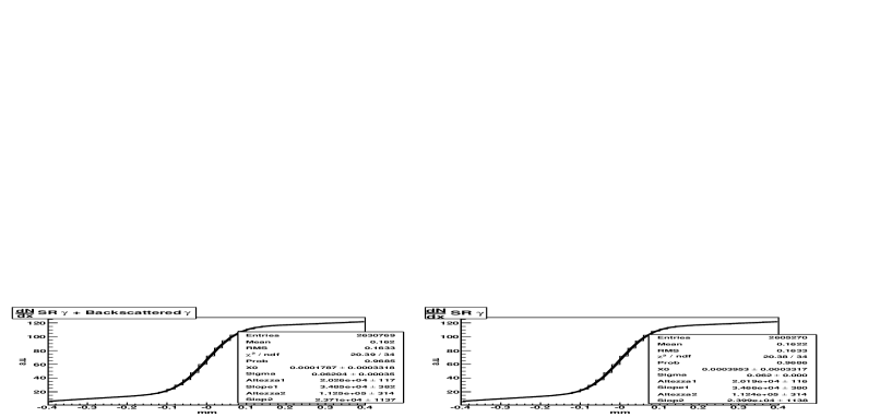
Figure 22: Left: Response function of the avalanche SR edge detector for all signal and background photons. Right: Response function of the same detector for only SR signal photons. The curves are the results of a fit of eq.(33) supplemented by an additional background tail.

well recognized and a fit using eq.(33) provides $X_{\gamma}=0.18\pm$ 0.33 $\mu$m. This number is, despite of the crudeness of the simulation, in perfect agreement with the demands and indicate that the response of Compton photon as background is not important. Hence, $X_{\gamma}$ position measurements can be performed with an avalanche SR detector as proposed in [43]. Presently, R&D for such a detector is ongoing and first results are expected in 2008/09 [50].

3.9 Laser Power

So far we assumed $10^{6}$ Compton interactions per crossing regardless of the laser type used. To achieve such an event rate, the required laser power is estimated as follows. Utilizing for the incident electron beam transverse bunch sizes of $\sigma_{x}$ = 20 $\mu$m, $\sigma_{y}$ = 2 $\mu$m and 300 $\mu$m in longitudinal direction at the Compton IP, for the transverse laser spot size 100 (50) $\mu$m in the case of an infrared (green) laser, a pulse duration of 10 ps, a crossing angle of 8 mrad and $2\cdot 10^{10}$ electrons per bunch, the infrared laser $e\gamma$ luminosity per crossing is according to eq.(12) evaluated to 0.166 per millibarn and $\mu$J, while a green laser provides 0.307 mb${}^{-1}\mu$J^-1 . If these luminosities are combined with the corresponding Compton cross section of $\sigma$ = 197.9 mb, respectively, 137.7 mb, a bunch related laser power of 30 or 24 mJ is obtained. At present, such lasers that match the pattern of the incident electron bunches are not commercially available. But the FLASH collaboration [17, 18], employing a laser in the infrared region with good reliability, and ongoing R&D for green lasers within the ILC community [8] will set milestones in the future, from which this proposal could greatly benefit.

3.10 Potential Background Processes of Electron to Photon Conversion

Usually, the characteristics of Compton scattering are calculated within the Born approximation, see Sect.2 as an example. Compton scattering processes at the ILC with large bunch densities, large laser flash energies and small pulse lengths ensure sufficient $e\gamma$ luminosity, which is important for precise $E_{b}$ determination. When the thickness of the laser target is about one collision length as at the ILC, each electron may undergo multiple Compton scattering within the crossing region [51]. The probability might not be small because, after a large energy loss in a first collision, the Compton cross section increases and together with the high particle densities of the colliding bunches further collisions can be caused. Such multiple scattering leads also to a low energy tail in the energy spectrum of the scattered electrons and could modify the sharp edge behavior. Using the program package CAIN [52] the rate of electrons which scatter more than once compared to single scatters has been conservatively evaluated to $\sim$0.7$\cdot 10^{-4}$, utilizing default beam parameters and a $CO_{2}$ laser with a pulse power of 1 mJ. Thus, out of $10^{6}$ Compton scatters only a small fraction undergoes multiple scattering. The disturbed energy spectrum is displayed in Fig. 24, while the position distribution of the electrons 50 m downstream of the magnet in Fig. 24. No significant distortion of the recoil electron spectra is expected.

Figure 23: Energy spectrum of Compton electrons including multiple scattering for a $CO_{2}$ laser at 250 GeV beam energy.

Figure 24: Position spectrum of Compton electrons 50 m downstream of the default magnet for a $CO_{2}$ laser at 250 GeV beam energy.

For the calculation of the $e\rightarrow\gamma$ conversion efficiency, one has besides geometrical properties of the laser and the Compton effect also to consider so-called nonlinear effects in the scattering process. Since the field in the laser wave at the crossing region can be very strong, electrons have a chance to interact simultaneously with several laser photons (called nonlinear QED effects). These nonlinear effects are characterized by the parameter [53]

$$\xi^{2}=\frac{2n_{\gamma}\cdot r_{e}^{2}\cdot\lambda}{\alpha_{fsc}}~{},$$ (34)

where $n_{\gamma}$ is the density of the laser photons, $r_{e}$ the classical electron radius, $\lambda$ the laser wavelength and $\alpha_{fsc}$ the fine structure constant. At $\xi^{2}\ll 1$, the electron scatters on only one laser photon, while at $\xi^{2}\gg 1$ on several.

The transverse motion of an electron in the electromagnetic wave leads to an effective increase of the electron mass and the maximum energy of the scattered photon decreases as $E_{b}\cdot x/(1+x+\xi^{2})$, with x given by eq.(2). Thus, with growing $\xi^{2}$ the energy spectrum of the Compton electrons will be modified in two respects, (i) the spectrum is shifted to higher energies and (ii) higher harmonics appear. Simulations with CAIN showed that for a $CO_{2}$ laser with 1 mJ pulse power, $\xi^{2}=1.04\cdot 10^{-5}$, so that within $10^{6}$ Compton events about 10 electrons absorb two photons at the same time. The relative shift of the edge energy is estimated to $3.2\cdot 10^{-6}$, a value practically not accessible by any of the detection systems proposed.

Besides nonlinear QED effects higher order QED corrections may also affect the electron endpoint behavior. In order to study such corrections the Compton electron energy cross section has been calculated for the complete order-$\alpha_{fsc}^{3}$ approximation and compared with the Born cross section in Fig. 25. The computer code used relies on Ref.[54]. The spectra shown assume Compton scattering of 500 GeV polarized electrons with green laser pulses of $P_{e}\lambda$ = -1. Such conditions allow for largest higher order contributions. As can be seen, the $e\gamma\rightarrow e\gamma$ Born approximation (black histogram) and the Born plus order-$\alpha_{fsc}^{3}$ correction cross section (open histogram) are very close to each other. The inclusion of the process $e\gamma\rightarrow e\gamma\gamma$ enhances the spectrum by about 5% (shaded histogram) without, however, a measurable shift of the endpoint value. The application of the code for the $e^{-}e^{+}e^{-}$ final state indicates that the minimum electron energy is about 34.4 GeV, i.e. $e\gamma\rightarrow ee^{+}e^{-}$ contributions are expected far outside of the region of interest.

In addition, with an increase of the variable x (eq.(2)), $e^{+}e^{-}$ pair creation by high energy Compton photon collisions with laser photons leads to further background, which has the potential to disturb edge electron characteristics. If x is larger than 4.83 which happens when e.g. 250 GeV electrons collide with green laser light, associated $e^{\pm}$ pair background is generated. For beam parameters and laser pulse power as mentioned above, CAIN provides about 18 $e^{+}e^{-}$ background pairs for $10^{6}$ Compton events. Besides this negligible event rate, the energy of such $e^{\pm}$ background particles is far away from the energy of the edge electrons.

These preliminary results indicate that effects as discussed will not affect the properties of the edge electrons and the backscattered $\gamma$-rays in a measurable manner.

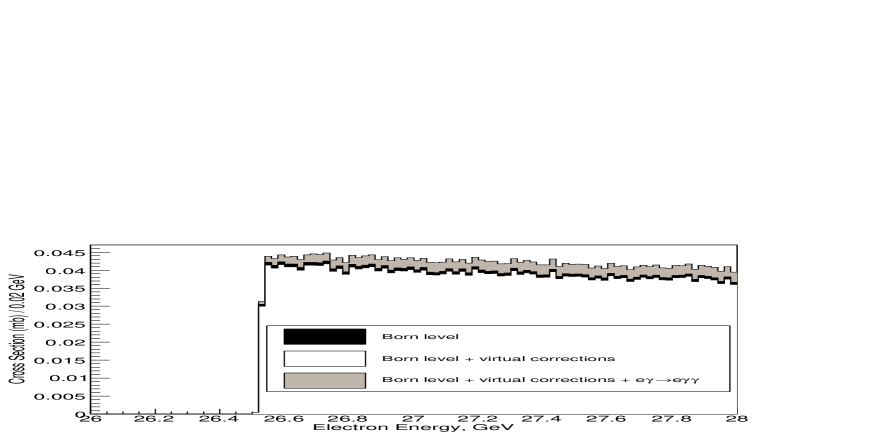
Figure 25: Born cross section of the Compton process (black histogram), Born plus order-$\alpha_{fsc}^{3}$ correction cross section (open histogram) and the Born plus order-$\alpha_{fsc}^{3}$ correction cross section including the reaction $e\gamma\rightarrow e\gamma\gamma$ (shaded histogram) with $P_{e}\lambda$ = -1 at 500 GeV.

3.11 Error Discussion and Calibration Issues

Concerning the statistical error, it has been shown that with $10^{6}$ Compton events per bunch crossing the accuracy on the beam energy $\Delta E_{b}/E_{b}$ can be brought well below the requirement of $10^{-4}$.

Different sources of potential systematic errors may affect the measurement of $E_{b}$ and are discussed below. As outlined in Sect.3.10, Compton processes beyond Born approximation such as multiple scattering, nonlinear effects in the $e\rightarrow\gamma$ conversion process, higher order QED corrections or $e^{+}e^{-}$ pair creation will not significantly modify the scattered photon and edge electron behavior. As shown by simulation, their effect on $\Delta E_{b}/E_{b}$ is negligible even after summation over all non-Born approximations discussed.

Variations of the transverse profile of the incident electron or laser beam and the angular spread as given in Sect.3.8 by a factor 2 or assuming a rectangular beam shape instead of a Gaussian do not modify the positions of the Compton photons and edge electrons in a measurable manner as long as both beams collide centrally. This means, $E_{b}$ determination by Compton scattering is rather robust against initial state beam variations.

Relying on method A, $\Delta E_{b}/E_{b}$ is controlled by the accuracy of the integrated B-field of the spectrometer magnet, $\Delta B/B$, the drift distance to the detector plane, $\Delta L/L$, and the offset of the edge position with respect to the primary beamline, $\Delta D/D$, see eq.(17) and Fig. 10. The drift distance can be precisely monitored using an interferometer [55]. For an accuracy of $\Delta L$ $\simeq$100 $\mu$m, which is feasible, the relative error of L becomes few times $10^{-6}$ and hence negligible. The required accuracy for the distance between the undeflected beam and the endpoint in the order of few micrometers is only possible when a $CO_{2}$ laser is used. To achieve such a precision the $X_{\gamma}$ and $X_{edge}$ detectors should be installed on a common frame and rigidly connected in order to avoid relative position movements. In this way and with a frame made out of a material with a small expansion coefficient like carbon the relative distance error between both devices can be kept below 1 $\mu$m [56], even with a $\pm 5^{o}$ change in tunnel temperature. More important contributions to $\Delta D/D$ constitute the uncertainties of the $X_{\gamma}$ and $X_{edge}$ position measurements themself. As discussed in Sect.3.8, the option to perform $X_{\gamma}$ measurements by means of a quartz fiber detector in conjunction with an adequate converter provides a statistical precision of 0.54 $\mu$m and the SR edge method 0.33 $\mu$m, while the total error should not exceed $\sim$1 $\mu$m, a challenging task.

The geometrical precision of quartz fibers is crucial for their precise assembly into plans and stacks. Arrangements of sufficient precisions including intrinsic fiber uncertainties are based on experience [39, 41, 42] and can be kept to 2 $\mu$m or better for small devices. The position of the fibers can be accurately measured after the assembly and recorded in a database for use during analysis so that final arrangement errors may be less than few tenth of a micrometer. Also, any tilt of the detector with respect to the vertical direction is important. For example, a misalignment error of 1 mrad could result to an $X_{\gamma}$ position shift up to 5 $\mu$m. Hence, the detector has to be aligned to better than 0.1 mrad in order to keep this bias contribution $\stackrel{{\scriptstyle<}}{{{}_{\sim}}}$0.2 $\mu$m.

Possible errors caused by the fit procedure of the escaping $e^{\pm}$ position distribution have been checked by varying the fit region within reasonable values or by rebinning the spectrum or by omitting the first step of the two-step fit procedure. There is no evidence found for a bias of the nominal fitted values, taking their statistical precision into account. Conservatively, we assign an error of 0.1 $\mu$m due to residual uncertainties from the fit.

The signal uniformity of the fiber sensor is also an important issue. Variations from fiber-to-fiber (or strip-to-strip) may have variuos reasons. There are statistical variations due to noise and fluctuations of the number of photons emitted, but also variations of the signal response laterally across the detector which are caused by fluctuations in the local properties of the sensor. Cerenkov light variations were already addressed in the GEANT simulations. The remaining fluctuations were studied by some additional Gaussian channel-to-channel signal variation of 0.5%, 1% and 2% of the total signal per fiber. It was found that the original position of interest is shifted by less than 1 $\mu$m for a response fluctuation not exceeding 1%. In practice, the level of uniformity across the sensor should be measured by an appropriate uniform illumination with particle beams and the individual channel response accounted for in the data analysis.

Imperfections within the fiber readout chain are difficult to estimate at the present stage of the project. However, in order to fulfill the request we set a limit of 0.2 $\mu$m for fiber-to-fiber signal variation respectively instability.

Alternatively, recording the SR edge by means of the avalanche detector [43], the primary beamline position depends on the amount and shape of the fringe field of the magnet. If the 1% integrated B-field fraction for the fringe field as used in the simulation was varied between 0.5 and 2% and three field shapes are considered (a simple step function, a straight line between zero and the B-field strength and a Gaussian distribution) it was found that the edge positions were distributed over a range of 1.6 $\mu$m. Thereby, precise measurement of the fringe field is mandatory, in particular upstream of the magnet. We estimate a residual error of $\sim$0.2 $\mu$m for $X_{\gamma}$ due to surviving uncertainties of the integrated B-field which includes imperfections of the fringe field. Also, additional errors of 0.1 and 0.2 $\mu$m due to imperfections in the fit procedure, respectively, electronics were assigned.

Since the beam and the laser widths are comparable in size, the laser has to be steered onto the electrons such that both beams collide centrally. Otherwise, a shift of the center-of-gravity of the scattered photons is generated. Options for laser spot size monitoring and its stabilization are discussed in Sect.3.6.2. Electron position and emittance are supplied by BPMs, respectively, wire-scanner systems distributed within the BDS. Beam jitter studies suggest for $\sigma_{jitter}$ = (0.1-0.5)$\cdot\sigma_{x(y)}$ [44, 57], where $\sigma_{x(y)}$ is the bunch size in x(y)-direction. For a beam extension $\sigma_{x}$ = 20 $\mu$m for example, the horizontal jitter is small, in the order of few micrometer, and negligible in the vertical direction. If one restricts any shift of $X_{\gamma}$ to be less than 0.3 $\mu$m, constraints for the beam displacement from one another as a function of the laser spot size can be derived. With $\sigma_{x}$ = 20 $\mu$m and a displacement of 15 $\mu$m, the laser spot size has to be $\sim$150 $\mu$m, or the position of the laser has to be stable within 12 $\mu$m. Larger spot sizes relax this condition, whereas a bigger electron bunch size aggravates the condition considerably. For example, a 50 $\mu$m bunch requires a laser spot of the order of 300 $\mu$m and a laser jitter of less than 10 $\mu$m in order to maintain the photon centroid shift below 0.3 $\mu$m. Luminosity loss due to larger laser spot sizes can be compensated by either an increase of the laser power or an increased pulse length, or a combination of both. If the pulse duration is substantially increased it seems of advantage to consider horizontal instead of vertical beam crossing. In conclusion, in order to design a laser system which restricts the shift of $X_{\gamma}$ due to non-central collisions of electron and laser pulses to less than $\sim$0.3 $\mu$m some R&D effort is needed.

Summing all contributions quadratically, the total error associated to the $\gamma$-ray centroid position is $\Delta X_{\gamma}$ $\simeq$ 0.8 $\mu$m for the quartz fiber detector-converter system, while the SR edge approach provides $\sim$0.6 $\mu$m. Both uncertainties are smaller than the required figure of $\sim$1 $\mu$m.

Concerning the measurement of the electron endpoint, we found for $X_{edge}$ an uncertainty of about 4 $\mu$m for the $CO_{2}$ laser (not discussed), while the infrared (green) laser provides values of 5 and 9 (12 and 15) $\mu$m for the DSD, respectively, QFD detector. The differences in precision are mainly due to different event rates per detector strip or fiber.

For the diamond strip detector we assume a similar alignment precision as for the $X_{\gamma}$ fiber detector discussed above and a bias estimate of 1.5 $\mu$m due to imperfections of the detector response.

The yield of the Cerenkov light in quartz fibers varies considerably in the vicinity of the Compton edge. Here, the number of incident electrons per fiber ranges from $\sim$150 to only a few or zero. Correspondingly, the number of photoelectrons in the light signal detector also varies considerably, which in turn requires high quantum efficiency at the wavelength of maximum scintillation and excellent single-photon detection capability. If we e.g. assume a zero-signal for fibers with less than 10 incident electrons, the refitted endpoint positions were found to be within $\pm$0.6 $\mu$m compared to the original values. This suggests to assign a total uncertainty associated to detector effects of 2 $\mu$m.

As emphasized in Sect.3.2, the relative error of the B-field integral should be close to $2\cdot 10^{-5}$ in order to reach the required beam energy precision. Sect.3.5 summarizes aspects necessary to fulfill this challenging request, and more details can be found in Ref.[1]. Here we point out that, independent of the endpoint detector utilized, in addition to the bending field provided by the spectrometer dipole itself, several other sources of magnetic fields may be present in the ILC tunnel which might influence the path of the electrons. A large effect can come from the earth’s field and other contributions might arise from cables which provide current for magnets. Such fields within the space between the Compton IP and the detector plane could spoil the endpoint position measurement, even if this space is free of any magnetic element. The effect of e.g. the earth’s field if normal to the full edge electron trajectory will shift the impact point 25 m downstream of the magnet by approximately 12 $\mu$m. Hence, the ambient field can be critical and should be either shielded or measured by e.g. a fluxgate magnetometer. Such an instrument allows to monitor any variation of the ambient magnetic field with time and endpoint corrections should be applied. It is estimated that such a field has to be known with a relative accuracy of (better than) 10% to ensure a tolerable contribution of $\stackrel{{\scriptstyle<}}{{{}_{\sim}}}$1.5 $\mu$m to the overall $X_{edge}$ uncertainty.

Adding all uncertainties together, the total error of $X_{edge}$ can be expected to be close to 5.6 or 9.3 $\mu$m (12.2 or 15.2 $\mu$m) if an infrared (green) laser is used in the spectrometer. The dominating fraction of the error comes from statistics so that larger data samples would decrease these uncertainties. In general, all estimated uncertainties are very close to or less than the errors anticipated in Sect’s.3.2 and 3.3.

If method B will be realized, precise position of the unscattered beam, $X_{beam}$, at the detector plane is also required. Cavity beam position monitors with single-bunch resolution of few hundred (or less) nanometers are best suited. To be conservative, we assume an error for $X_{beam}$ of 1 $\mu$m which has to be added in quadrature with the uncertainty from possible charged particle background expected for one of the proposed spectrometer locations (Sect.3.12). In the worst case, the total uncertainty of $X_{beam}$ results to $\sim$1.2 $\mu$m which is well within the requirement.

In addition, if the B-field integrals for the endpoint and beam electrons are different, ${(\int Bdl)}_{edge}\neq{(\int Bdl)}_{beam}$, the expression for the beam energy (25) must be rewritten as

$$E_{b}\propto\frac{R(X_{edge}-X_{\gamma})-(X_{beam}-X_{\gamma})}{(X_{beam}-X_{\gamma})}~{},$$

with

$$R=\frac{{(\int Bdl)}_{beam}}{{(\int Bdl)}_{edge}}~{}.$$

Hence, the error for the beam energy as a function of the relative uncertainty of R is

$$\frac{\Delta E_{b}}{E_{b}}=\frac{(X_{edge}-X_{\gamma})}{(X_{edge}-X_{beam})}\frac{\Delta R}{R}~{},$$

where the approximation $R\approx 1$ has been implied. If the corresponding particle positions 25 m downstream of the spectrometer magnet are taken into account, the ratio $\frac{(X_{edge}-X_{\gamma})}{(X_{edge}-X_{beam})}$ = 1.2 (1.1) for the infrared (green) laser. This means that for $\frac{\Delta R}{R}\simeq 5\cdot 10^{-5}$ or better and any value of $R$ different from 1, eq.(25) is needed to be modified as indicated above. If $R$ equals 1 (within few times $10^{-5}$) no correction has to be applied. With today’s common B-field and $\int Bdl$ measurement techniques such precision for $R$ can be achieved without too much efforts.

Basically, whatever will be the final choice for the detector more elaborated simulation studies are mandatory. In particular, physics processes in the sensor material, basic parameters of the associated electronics and backgrounds need to be taken into account. Such details may affect the edge position and its shape and could limit the performance of the spectrometer. Studies of this kind are, however, beyond the scope of this paper.

The idea to pulse the laser on every ILC bunch may be diluted for background studies. If e.g. the laser is pulsed on nine out of ten bunches, every 10th pulse can be used for background studies. Also, when the laser fires without beams, checks of, for example, possible pick-ups in the electronics can be performed.

The experience at SLC and LEP proved that independent measurements of the beam energy are important. The canonical method to measure $E_{b}$ upstream of the $e^{+}e^{-}$-IP consists of the BPM-based spectrometer [1]. Both the Compton and the BPM-based spectrometers are designed to provide an absolute measurement of the beam energy with a relative accuracy of $10^{-4}$. Cross-calibration of the spectrometers would provide an important and valuable control of their systematic errors. Also, energy measurements at the $Z$-pole would provide a unique possibility for an early calibration in a well understood physics regime. Although $Z$-pole calibration measurements are not part of the current ILC baseline design [44] it is argued [58] that the baseline should be modified to include such reference. In addition, physics reference channels, such as $e^{+}e^{-}\rightarrow\mu^{+}\mu^{-}\gamma$ where the muons are resonant with the known $Z$-mass, are foreseen to provide valuable checks of the collision energy scale, but only long after the data were recorded.

3.12 Suitable Spectrometer Locations

Although the today’s beam delivery system [11] will be further developed within the next years, basic properties are not expected to be modified. We propose three alternatives for possible locations of the Compton spectrometer within the BDS, while keeping major design parameters of the spectrometer unaltered. Each of the proposals has pros and cons and the spectrometer viability requires sometimes, depending on the location, slight modifications of the present BDS. An overall view of the BDS is shown in Fig. 26, where also potential locations for the Compton spectrometer are indicated.

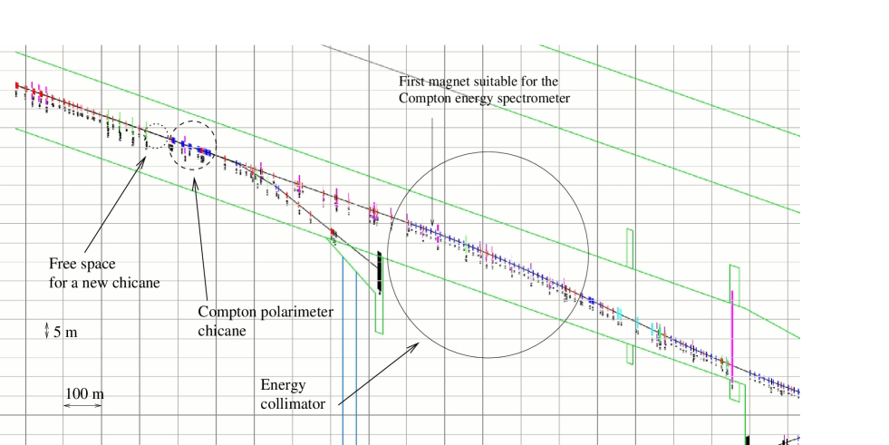
Figure 26: General view of the beam delivery system with possible locations of the Compton spectrometer.

Common to all alternatives is the demand to locate the spectrometer upstream of the energy collimation system to avoid significant muon background excess relative to the rate from normal collimation losses.

The straight-forward approach suggests to locate the spectrometer in an existing free-space region of the BDS. The amount of space needed is determined by the drift distance of at least 25 m to the detector system, the length of the magnet of 3 m and the 6 m long vacuum chamber upstream of the dipole in which the Compton IP is contained. The sum of these components of 35 m has to be enlarged by additional space to accommodate two ancillary magnets with corresponding drift regions to compensate the bend of the spectrometer magnet. Hence, in total 60-70 m free space is needed. Far upstream of the physics $e^{+}e^{-}$-IP such free space of some 65 m exists, see Fig. 26. The transverse dimensions of the beam at the Compton IP of about 20 $\mu$m versus 2 $\mu$m perfectly match the expected spot size of the laser. Additional muon background generated by backscattered electron interactions further downstream was estimated and would only increase the muon rate by a small amount [59], independent of the laser wavelength. This suggestion locates the spectrometer on a direct line of sight to the main linac, which means that backgrounds in this region are likely to be significant. In particular, charged particles off in energy may affect the position of the beamline in the cavity BPM. Cavity beam position monitors measure the centroid of the particle’s charge distribution and, hence, particles with less energy than $E_{b}$ are stronger deflected by the spectrometer magnet and could shift the measured beam position. Halo and tail generation estimates based on simulation [60] reveal that at the exit of the linac the beam profile is superimposed by a symmetric halo extending to about $\pm$300 (50) $\mu$m in x(y)-direction. The fraction of particles off in energy was estimated to be few times $10^{-5}$ with a broad energy spectrum that sharply peaks very close to the nominal beam energy. A simple tracking procedure up to the BPM installed 25 m from the spectrometer magnet indicates a shift of $X_{beam}$ of 0.65 $\mu$m which we consider of not being catastrophic. It is also estimated that this background does not affect the Compton endpoint position in a significant manner. The synchrotron photons from the quadrupole fields within the linac and the beginning of the BDS have a $\sim 10^{2}$ times lower critical energy [60, 61] than those from the spectrometer magnet and are considered to be of no serious issue. However, due to the uncertainties in the charged particle background simulation it is favorable to locate the spectrometer after a protective bend, so that the beam position will be much less impacted.

A major constraint for the design of the Compton spectrometer is the synchrotron radiation emittance dilution from the additional spectrometer magnets. Employing the magnet as discussed in Sect.3.3 and similar ancillary magnets, an emittance growth of about 0.5% at 250 GeV is expected, which might be considered as acceptable. Since the emittance scales with the sixth power of the beam energy, further studies have to reveal whether emittance dilution at 500 GeV beam energy can be tolerated.

A second option for the spectrometer location consists in employing one or more magnets of the present BDS as the Compton spectrometer dipole. Since, however, an individual magnet with desirable properties does not exist, we suggest to combine several consecutive bending magnets. At the beginning of the energy collimation section directly after the first magnet, see Fig. 26, such magnets might be combined to provide the desired bending power. In particular, if the laser IP is located about 3 m upstream of magnet 1, a combination of the following six magnets (magnet 1, …, magnet 6) provides sufficient particle separation. For example, separation between the backscattered $\gamma$-rays and the beamline results to 18 mm after passing magnet 6, while the distance of the beam to the edge electrons is 26 mm for a $CO_{2}$ and 98 mm for an 1.165 eV infrared laser. Thus, by locating the detector system close to magnet 7 convenient measurements of the positions of the Compton recoil particles and the beamline can be performed. The transverse beam profile at the laser IP is sufficiently small so that the beam is completely covered by the laser spot. Additional muon background from Compton electrons is tolerable since many of these electrons will hit either closely located magnets or spoilers of the energy collimation system [59]. This option also allows to insert the laser light into the vacuum pipe downstream of magnet 1 which makes strict head-on collisions with the beam possible.

However, the horizontal aperture of the magnets has to be continuously increased towards the bending direction so that the edge electrons pass in B-fields with properties as demanded. In particular, at the exit of magnet 6 the vacuum chamber has to have a horizontal aperture of 115 mm for infrared laser light scattering. Furthermore, if method A is employed for beam energy measurements, the B-field integral over all six magnets has to be known with 20 ppm precision. Or, for method B, the three-point measurement approach, sufficient field uniformity uncertainty within the bending plane up to x = 115 mm has to be ensured. Whatever method for $E_{b}$ determination will be realized, the demands for the magnet system are challenging. This alternative for the spectrometer location is advantageous since no additional magnets are needed and, thereby, further growth of the beam emittance is a priori avoided.

The third alternative for a location of the Compton spectrometer consists in employing the magnetic chicane proposed for high energy polarization measurements [9]. In particular, the four-magnet polarimeter chicane with the laser IP in the mid-point is supposed to be supplemented by the position sensitive detector system, which should be located upstream but close to the fourth magnet. Also, some dedicated adjustments of space, laser and detector conditions are needed to ensure polarization and beam energy measurements simultaneously with precisions as anticipated. However, the present baseline polarimeter design aims to operate the chicane with constant field settings over a large range of beam energies, while the Compton based beam energy spectrometer intends to adjust the B-field to a constant bending power of e.g. 1 mrad. Whether both approaches can be merged to a common proposal requires detailed studies. Possible muon background increase from Compton electron interactions was estimated to be tolerable [59]. It is also obvious that additional dilution of the beam emittance caused by such $E_{b}$ measurements is ruled out.

4 Summary and Conclusion

A novel, non-invasive method of measuring the incident beam energy, $E_{b}$, at the International $e^{+}e^{-}$ Linear Collider is proposed. Laser light scatters head-on off ILC bunches and generates Compton electrons and photons. After the Compton IP, the scattered particles as well as the non-interacting beam electrons (99.9995% of them) pass through a dipole magnet so that further downstream access to each particle type is possible. $E_{b}$ measurements can be performed continuously on a bunch-by-bunch basis while the electron and positron beams are in collision.

One approach to infer $E_{b}$, method A, relies on the beam energy dependence of the momentum of the scattered electrons at the kinematic endpoint, the edge energy. Combining the B-field integral of the dipole with the position of the edge electrons relative to the incident beam provides the energy of the edge electrons and, thereby, $E_{b}$. However, integrated field uncertainties close to $2\cdot 10^{-5}$ and position measurements with an accuracy of at least few micrometers are required to achieve the anticipated value of $10^{-4}$. The last demand is very challenging and is mainly the reason to follow a different approach, called method B. By measuring three particle positions, the position of the Compton scattered $\gamma$-rays, $X_{\gamma}$, the position of the edge electrons, $X_{edge}$, and that of the beam, $X_{beam}$, downstream of the spectrometer magnet allows to deduce $E_{b}$ with precisions of $10^{-4}$ or better. Such precisions, however, require to measure the distance $X_{edge}-X_{beam}$ with an accuracy of about ten micrometer and $X_{\gamma}$ with 1-2 $\mu$m uncertainty. Both requirements seem to be achievable, because the distance $X_{edge}-X_{beam}$ is, in particular, beam energy independent and accumulation over many bunches decreases its statistical error substantially.

It has been shown that effects beyond the Born approximation in the laser crossing region are very small. They only lead to a negligible shift of the edge electron position, $X_{edge}$.

Geometrical constraints and acceptable emittance dilution of beam particles when passing the dipole magnet require a spectrometer length of at least 30 m. The geometrical constraints in conjunction with free space options within the beam delivery system preclude the usage of a $CO_{2}$ laser, while an infrared (with $E_{\lambda}$ = 1.165 eV) or a green laser (with $E_{\lambda}$ = 2.33 eV) are both suitable. To achieve e.g. $10^{6}$ Compton events per bunch crossing, a pulse power of 30 mJ, respectively, 24 mJ with a pattern that matches the pulse and bunch structure at the ILC is needed. Such lasers are presently commercially not available, but R&D is ongoing within the ILC and other communities.

For particle position measurements, detectors with high spatial resolution have to be pursued. As a promising option for edge electron and $\gamma$-ray center-of-gravity measurements quartz fiber detectors are suggested because they are very radiation hard and ultrafast. An alternative to the $X_{\gamma}$ quartz fiber detector (in conjunction with e.g. a 16 radiation length tungsten converter) consists in measuring the edge position of synchrotron radiation light generated by beam particles when passing the spectrometer magnet, as discussed in [43]. A device based on gas amplification was considered in more details and simulations demonstrated its reliability for our purpose. The position of the non-interacting beam particles needs to be known with micrometer accuracy which can be relative easily achieved by modern cavity beam position monitors.

The method proposed to perform energy measurements of the incident beam at the ILC is thought to be a complementary and cross-check approach to the canonical concept of a BPM based energy spectrometer. Both methods intend to achieve a precision of $10^{-4}$ on a bunch-to-bunch basis. The method studied in this paper seems to accomplish the objective, but more detailed studies are mandatory and a prove-of-principle experiment [62] should to be performed to test the three-position measurement approach.

Acknowledgment

We would like to thank A. Magaryan for discussions, where the idea of the present study originated. We would also like to thank K. Hiller, R. Makarov, N. Morozov and E. Syresin for helpful discussions and the sommerstudents H. Paukkunen, J. Lange and D.A. Stüken for various contributions. We are grateful to L. Keller for performing muon background calculations, A. Latina for bunch simulations within the ILC, H. Burkhard for halo and tail information, G. Klemz for discussions on laser system aspects and G.A. Blair for reading the manuscript.

References

-
[1]
V.N. Duginov et al., The Beam Energy Spectrometer
at the International Linear Collider, LC-DET-2004-031;
M. Hildreth et al., SLAC T-474, June 2004. - [2] R. Assmann et al., Eur. Phys. J. C39 (2005) 253, CERN-PH-EP-2004-032 and CERN-AB-2004-030 OP.
-
[3]
J. Kent et al., SLAC-PUB-5110 (1990);
S. Herzbach, Proc. of the International Linear Collider Workshop, Batavia, Illinois, USA, October 2000. -
[4]
K. Hiller et al., EUROTeV-Report-2006-091;
P. Galmian et al., Nucl. Instr. Meth. A327 (1993) 269;
C. Checchi, J.M. Field and T. Kawamoto, Nucl. Instr. Meth. A385 (1997) 445;
V.I. Telnov, 26th Advanced ICFA Beam Dynamics Workshop on Nanometer Colliding Beams - Nanobeam 2002, p.159, Cern-Proceedings-2003-001, 2-6 September 2002, Lausanne, Switzerland;
D.P. Barber and R.A. Melikian, Proc. of EPAC 2000, Vienna, 2000;
R.A. Melikian and D.P. Barber, DESY 98-015 (1996) and hep-ph/9903007. - [5] Ian C. Hsu, Cha-Ching Chu and Chuang-Ing Yu, Phys. Rev. E54 (1996) 5657.
- [6] R. Klein et al., Nucl. Instr. Meth. A384 (1997) 293 and Nucl. Instr. Meth. A486 (2002) 545.
-
[7]
V.E. Blinov et al., Nucl. Instr. Meth. A 598 (2009) 23;
N. Muchnoi, S. Nikitin and V. Zhilich, Proc. of the EPAC 2006, Edinburgh, Scotland, 2006. -
[8]
see e.g. M. Ross, Laser-Based Profile Monitors for Electron Beams,
SLAC-PUB-8-57, Feb. 1999 and
Linear Collider Diagnostics, Proc. of Beam Instrumentation
Workshop, 0 MA, USA, 2000;
I. Agapov, G.A. Blair and M. Woodley, Phys. Rev. ST Accel. Beams, 10 (2007) 112801;
A. Bosco et al., EUROTeV-Report-2006-093 and Nucl. Instr. Meth. A (2008), doi:10.1016/j.nima.2008.04.012 ;
G.A. Blair, EUROTeV-Report-2006-009;
M.T. Price et al., EUROTeV-Report-2006-046. -
[9]
N. Meyners, V. Gharibyan and K.P. Schüler,
Proc. of the International Linear Collider Workshop, p. 871,
Stanford, California, USA, 18-22 March 2005;
K.O. Eyser et al., Proc. of the International Linear Collider Workshop, Hamburg, Germany, 28 May-01 June, 2007. -
[10]
see e.g. J. Ballam et al., Phys. Rev. Lett. 23 (1969) 498;
L. Federice et al., Nuovo Cimento B59 (1980) 247:
A. M. Sandorfi et al., IEEE Trans. Nucl. SCI. NS-30 (1983) 3083. -
[11]
A. Syryi et al., Proc. of PAC 2007, Albuquerque, New Mexico,
USA, June 25-29, 2007;
M. Woodley, European LC Workshop, Daresbury, England, January 8-11, 2007;
ILC BDS lattice online repository: http://www.slac.stanford.edu/ mdw/ILC/2006e/. - [12] E. Feenberg and H. Primakoff, Phys. Rev. 73 (1948) 459.
- [13] H.J. Schreiber, International Linear Collider Workshop, Valencia, Spain, 6-10 November 2006.
- [14] T. Suzuki, General formulae of luminosity for various types of colliding beam machines, KEK-76-3 (1976).
- [15] G. Bardin, C. Cavata and J. P. Jordan, Compton polarimeter studies for TESLA, DESY-TESLA-97-03.
- [16] T. Omori et al., Nucl. Instr. Meth. A500 (2003) 232.
- [17] I. Will, P. Nickles and W. Sander, A Laser System for the TESLA Photo-Injector, internal design study, Max-Born-Institut, Berlin, 1994.
- [18] S. Schreiber et al., Nucl. Instr. Meth. A445 (2000) 427 232.
- [19] N. Yu. Muchnoi, Proc. of the International Linear Collider Workshop, DESY, Hamburg, Germany, 28 May-01 June, 2007.
- [20] S. Walston et al., Nucl. Instr. Meth. A 578 (2007) 1.
- [21] D. Whittum and Y. Kolomenski, Review of Scientific Instruments, V. 70, N 5, May 1999.
- [22] M. Slater et al., SLAC-PUB-13031, EUROTeV-Report-2007-059 and arXiv:0712.1350v1; submitted to Nucl. Instr. Meth.
- [23] N.A. Morozov and H.J. Schreiber, Magnetic field calculations for the technical proposal of the TESLA spectrometer magnet, JINR communication - E9-2003-65, Dubna, 2003 and Meeting on BPM-based Beam Energy Spectrometer, DESY, March 17/18, 2003, http://www-zeuthen.desy.de/e_spec/Morozov.pdf.
- [24] N.A. Morozov, The preliminary estimation of the parameters for the TESLA spectrometer magnet, internal report, LNP JINR, Dubna, 2002.
- [25] N.A. Morozov, Calculations on optimization of the parameters for the TESLA spectrometer magnet, internal report, LNP JINR, Dubna, 2003.
- [26] N.A. Morozov, Magnetic field calculations for the TESLA spectrometer main magnet by the 3D MAFIA code, internal report, LNP JINR, Dubna, 2003.
-
[27]
N.A. Morozov, Review of the progress in the 2D and 3D magnetic field
simulation for the TESLA spectrometer magnets,
Meeting on BPM-based Beam Energy Spectrometer, Dubna, October 13-14, 2003,
http://www-zeuthen.desy.de/e_spec/morozov_magnets.pdf. - [28] M. Levi, J. Nash and S. Watson, Nucl. Instr. Meth. A 281 (1989) 265 and SLAC-PUB-4654, March 1989.
-
[29]
Encyclopedia of Laser Physics and Technology,
http://www.rp-photonics.com/gaussian_beams.html. - [30] A. Jerrard and M. Berch, Introduction to Matrix Optics, Moscow, Mir, 1978.
-
[31]
e.g. F. Stephan et al., Detailed characterization of electron sources
at PITZ yielding first demonstration of Europan X-ray Free Electron Laser beam quality,
submitted to Phys. Rev. Special Topics Acc. and Beam;
and G. Klemz, private communication. A. Jerrard and M. Berch, Introduction to Matrix Optics, Moscow, Mir, 1978. -
[32]
The RD42 Collaboration, CERN/EP 98-79;
W. Adam et al., Nucl. Instr. Meth. A 565 (2006) 278. - [33] P. Gorodetzki et al., Nucl. Instr. Meth. A 361 (1995) 101 and CERN-PPE/94-226.
- [34] The RD42 Collaboration, M. Barbero et al., CERN/LHCC 2008-005.
- [35] The RD42 Collaboration, W. Adam et al., Nucl. Instr. Meth. A 476 (2002) 706.
- [36] The RD42 Collaboration, M. Krammer et al., Diamond and Rel. Materials 10 (2001) 1778.
- [37] M.M. Zoeller et al., IEEE Trans. on Nucl. Sci. 44 (1997) 815.
- [38] J. Bol et al., IEEE Trans. on Nucl. Sci. 51 (2004) 2999.
-
[39]
N. Akchurin et al., Nucl. Instr. Meth. Phys. Res. A 399 (1997) 202
and Nucl. Instr. Meth. Phys. Res. A 408 (1998) 380;
I. Abt et al., Nucl. Instr. Meth. Phys. Res. A 386 (1997) 310;
R. Arnaldi et al., Nucl. Instr. Meth. Phys. Res. A 411 (1998) 1;
R. Amaldi et al., Nucl. Instr. Meth. Phys. Res. A 456 (2001) 248. -
[40]
e.g. W. Goettmann et al., Proc. of DIPAC 2005, Lyon, France;
R. Naka et al., IEEE Trans. on Nucl. Sci. 48 (2001) 2348;
R. Nishiara and N. Izumi, Mitsubishi Electronic ADVANCE (2001) 25;
E. Janata, Meth. Phys. Res. A 493 (2002) 1. -
[41]
e.g. H1-Collaboration, Proc. of the 28th Intern. Conf. on High
Energy Physics, Warsam, Poland, 1966, Vol. II, p. 1759;
R. Ansorge et al., Nucl. Instr. Meth. A 265 (1988) 33;
P. Annies et al., Nucl. Instr. Meth. A 367 (1995) 367;
A.D. Bross, Nucl. Phys. B (Proc. Suppl.) 44 (1995) 12;
D. Adams et al., Nucl. Phys. B (Proc. Suppl.) 44 (1995) 332;
A. Barcyk et al., Phys. Lett. B 663 (2008) 172. - [42] ATLAS collaboration, CERN/LHCC/2004-010, LHCC I-014, March 2004.
- [43] K. Hiller et al., Nucl. Instr. Meth. A 580 (2007) 1191 and LC-DET-2006-005.
-
[44]
B. Barish et al., ILC Reference Design Report (2007),
ILC-Report-2007-001,
http://www.linearcollider.org/cms/ . -
[45]
GEANT, Detector Description and Simulation Tool, CERN Program
Library Long Write-up, W5013, 1994;
S. Agostinelli et al. (GEANT4 Collaboration), Nucl. Instr. Meth. A 506 (2003) 250;
J. Allison et al., IEEE Trans. Nucl. Sci. 53 (2006) 270. - [46] e.g. S. Guiducci, private communication.
- [47] A. Latina, private communication.
- [48] P. Gorodetzki et al., Radiat. Phys. & Chem. 41 (1993) 253.
- [49] M. Morhac et al., Nucl. Instr. Meth. A 443 (2000) 108.
-
[50]
B. Zalikhanov, Meeting on Beam Energy Measurements, DESY Zeuthen,
November 21-23, 2005,
http://www-zeuthen.desy.de/e_spec/e_spec_nov21-2305.html;
R. Makarov, Meeting on Beam Energy Measurements, DESY Zeuthen, June 06-08, 2007, http://www-zeuthen.desy.de/e_spec/e_spec_jun06-0807.html;
E. Syresin, private communication. - [51] V.I. Telnov, Nucl. Instr. Meth. A 335 (1995) 3.
- [52] User’s Manual of CAIN, Version 2.35.
- [53] see e.g. V.B. Berestetskii, E.M. Lifshitz and L.P. Pitaevski, Quantum Electrodynamics, Pergamon Press, Oxford, 1982.
- [54] M.L. Swartz, Phys. Rev. D 58, 014010.
- [55] J. Gervaise, CERN 87-01 (1987) 128.
- [56] G. Barber et al., Nucl. Instr. Meth. A 254 (1987) 535.
- [57] A. Seryi, L. Hendrickson and G. White, 36th ICFA Advanced Beam Dynamics Workshop (NANOBEAM 2005), Kyoto, Japan, 2006.
- [58] B. Aurand et al., Excecutive Summary of the Workshop on Polarisation and Beam Energy Measurements at the ILC, ILC Note 2008-047.
- [59] L. Keller, private communication.
- [60] H. Burkhardt et al., EUROTEV-Report-2008-076; L. Neukermans, EUROTEV Meeting, Daresbury, January 8-9 2007: H. Burkhardt, private communication.
- [61] L. Deacon et al., EUROTEV-Report-2008-002-1.
- [62] N. Muchnoi and M. Viti, proposal in preparation.