CERN–PH–EP/2008–021

Dominik Dannheim^1ab, Tancredi Carli¹, Alexander Voigt¹,

Karl-Johan Grahn², Peter Speckmayer^3c

¹ CERN, Geneva, Switzerland

² KTH, Stockholm, Sweden

³ Technische Universität, Wien, Austria

Probability Density Estimation (PDE) is a multivariate discrimination technique based on sampling signal and background densities defined by event samples from data or Monte-Carlo (MC) simulations in a multi-dimensional phase space. In this paper, we present a modification of the PDE method that uses a self-adapting binning method to divide the multi-dimensional phase space in a finite number of hyper-rectangles (cells). The binning algorithm adjusts the size and position of a predefined number of cells inside the multi-dimensional phase space, minimising the variance of the signal and background densities inside the cells. The implementation of the binning algorithm (PDE-Foam) is based on the MC event-generation package Foam. We present performance results for representative examples (toy models) and discuss the dependence of the obtained results on the choice of parameters. The new PDE-Foam shows improved classification capability for small training samples and reduced classification time compared to the original PDE method based on range searching.

appeared in: Nucl. Inst. and Meth. A 606, 717 (2009)

 

^a Corresponding author; e-mail: dominik.dannheim@cern.ch.

^b Now with Max-Planck-Institut für Physik, München, Germany.

^c Now with CERN.

1 Introduction

Multi-variate discrimination techniques are used in high energy physics to distinguish signal from background events based on a set of measured characteristic observables. The information contained in the individual observables is combined into a single “discriminant” variable, on which then a cut is applied to separate signal from background. For an introduction to multi-variate discrimination techniques see e.g. Ref. [1].

Besides other approaches, non-parametric probability density estimaton (PDE) methods are used. Non-parametric PDE methods calculate a discriminant for each event to be classified based on the density of signal and background events in the vicinity of its coordinate in the multi-dimensional phase space. In the following we consider only methods that sample the event densities with probe volumes of fixed size. These methods have been used e.g. in searches for new physics at the Tevatron [2] and at HERA [3, 4] and for particle identification at the LHC [5].

A PDE method based on range searching (PDE-RS) [6] has been used successfully for classification problems in higher-dimensional observable spaces and with arbitrary correlations between the observables. Large samples of Monte-Carlo (MC) simulated signal and background training events are stored in binary-search trees. An efficient range-searching algorithm is used to sample the signal and background densities in small multi-dimensional boxes around the phase-space points to be classified. It handles the involved statistical uncertainties in a transparent way and has the size of the sampling box as the only free parameter.

An apparent limitation of PDE-RS, on the other hand, is the fact that large signal and background training samples are required to densely populate the multi-dimensional phase space. This is of particular importance in applications with many dimensions. Furthermore, these samples have to be accessible in the main memory of the computer used for the classification and the classification time scales with the number of training events like $T_{class}\propto N_{train}\cdot\log N_{train}$. Though adaptive resizing and kernel-convolution mechanisms for the sampling box have been implemented for PDE-RS in the toolkit for multi-variate data analysis with ROOT (TMVA) [7], the geometry of the sampling box is always identical in all dimension and it is therefore not optimally adapted to cases where the density distributions vary for the different dimensions involved.

In this paper, we propose an improvement of the original PDE-RS method [6] that reduces the sensitivity to statistical fluctuations of the training samples and results in a very fast and memory-efficient classification phase, independent of the size of the training samples. A self-adapting binning method is used to divide the multi-dimensional phase space in a finite number of hyper-rectangles (boxes). Only the binned density information is preserved in binary trees after the training phase, allowing for a very fast and memory-efficient classification of events. The implementation of the binning algorithm (PDE-Foam) is based on the MC event-generation package Foam [8].

2 Probability Density Estimation

PDE methods are based on the assumption that the probability for an event x (characterised by a set of $d$ observables $x_{1},...,x_{d}$) to belong to the signal class is given as a uniformly continuous function $P(\textbf{x})$. According to Bayes’ theorem, $P(\textbf{x})$ is derived from the probability density functions for signal and background, $\rho_{s}(\textbf{x})$ and $\rho_{b}(\textbf{x})$, and from the a-priori probabilities $p_{s}$ and $p_{b}$ for an event to be of class signal or background, respectively, as

$$P(\textbf{x})=\frac{\rho_{s}(\textbf{x})p_{s}}{\rho_{s}(\textbf{x})p_{s}+\rho_{b}(\textbf{x})p_{b}}.$$ (1)

The signal probability $P(\textbf{x})$ is a monotonously rising function of the Discriminant $D(\textbf{x})$:

$$D(\textbf{x})=\frac{\rho_{s}(\textbf{x})}{\rho_{s}(\textbf{x})+\rho_{b}(\textbf{x})}$$ (2)

in the relevant range $0\leq D(\textbf{x})\leq 1$, such that a cut on $D$(x) is always equivalent to a cut on $P$(x). $P$(x) and hence $D$(x) are the optimal discriminants according to the Neyman-Pearson lemma [9].

Estimates $\rho^{\prime}_{s}(\textbf{x})$ and $\rho^{\prime}_{b}(\textbf{x})$ of the signal and background probability density functions are obtained by sampling the $d$-dimensional phase space with events of known type. Such events can be either obtained from MC simulations or by defining data control samples in an appropriate way. The estimated discriminant:

$$D^{\prime}(\textbf{x})=\frac{\rho^{\prime}_{s}(\textbf{x})}{\rho^{\prime}_{s}(\textbf{x})+\rho^{\prime}_{b}(\textbf{x})})\approx D(\textbf{x})$$ (3)

approximates the true discriminant $D(\textbf{x})$ for sufficiently densely populated sampling space.

For any given combination of observables, x, the discriminant $D^{\prime}(\textbf{x})$ assigns a single value, which allows to discriminate background from signal events. In the framework of a physics analysis, a cut on a particular value of $D^{\prime}$ is applied, depending on the required purity and efficiency of the event selection. The signal and background probability density functions have to be approximated with sufficient accuracy. This poses a challenging problem in particular for high-dimensional cases.

A solution based on range searching (PDE-RS [6]) counts the number of MC generated signal and background events in the vicinity of each event to be classified. The discriminant $D^{\prime}(\emph{x})$ is defined from the number of signal events $n_{s}$ and the number of background events $n_{b}$ in a small volume $V(\textbf{x})$ around the point x:

$$D^{\prime}(\textbf{x})=\frac{n_{s}}{n_{s}+c\cdot n_{b}}.$$ (4)

The normalisation constant $c$ has to be chosen such that the total number of simulated signal events, $N_{s}$, is equal to $c$ times the total number of background events, $N_{b}$:

$$N_{s}=c\cdot N_{b}$$ (5)

The statistical uncertainty on the value of the discriminant $D$ is obtained from a propagation of the uncertainty on the number of events contained in the counting volume:

$$\sigma_{D}^{\prime}(x)=\sqrt{\left(\frac{c\cdot n_{b}}{(n_{s}+c\cdot n_{b})^{2}}\sigma_{n_{s}}\right)^{2}+\left(\frac{c\cdot n_{s}}{(n_{s}+c\cdot n_{b})^{2}}\sigma_{n_{b}}\right)^{2}},$$ (6)

where $\sigma_{n_{s}}$ and $\sigma_{n_{b}}$ are the statistical uncertainties of the number of signal and background events respectively.

$D^{\prime}(\textbf{x})$ provides a good estimate of $D(\textbf{x})$ for sufficiently small probe volumes $V(\textbf{x})$ and large numbers of MC simulated sample events. Figure 1(a) shows the distribution of the discriminant $D^{\prime}(x)$ for signal and background testing events of an arbitrary example. The discriminant takes values between 0 and 1. Most signal events are found at large values of $D^{\prime}$, while the distribution for background events peaks at small values of $D^{\prime}$. A given cut value $D_{c}$ results in an efficiency for signal and background testing samples, $\epsilon_{s}(D_{c})$ and $\epsilon_{b}(D_{c})$. Figure 1(b) shows the relation between signal efficiency $\epsilon_{s}$ and background rejection $1-\epsilon_{b}$ when scanning all values of $D_{c}$ between 0 and 1. The area under this so called Receiver operating characteristic (ROC) is a measure of the average estimator performance. A value of 0.5 is obtained for a random classification of signal and background. A value of 1.0 is obtained for a perfect discrimination between signal and background. For the example shown in Fig. 1, the obtained ROC value is 0.88.

The optimal performance measure for a particular practical application has to be chosen according to the desired balance between purity and efficiency. In high energy physics, MVA methods are often used in searches for rare events, where a small signal is overwhelmed by background. In such cases, the signal efficiency for a given large value of the background rejection is a more relevant performance measure than the overall area of the ROC curve. In addition to the ROC area, one therefore often quotes $\epsilon_{S,R=99\%}$, the signal efficiency at a background rejection of 99%. For the example shown in Fig. 1, the resulting value is $\epsilon_{S,R=99\%}=13.0\%$.

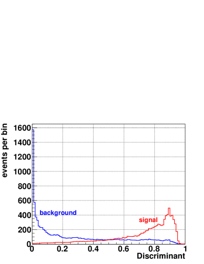
(a) Discriminant distribution

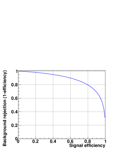
(b) Receiver Operating Characteristic

Figure 1: (a) Distribution of the discriminant for an arbitrary example of signal and background MC events. (b) ROC curve for the same example. The area under the curve characterises the performance of the estimator.

3 Adaptive phase-space binning with Foam

In the following we propose an alternative method to calculate the discriminant $D(\textbf{x})$ based on a binned sampling of the phase space.

Simple binning methods often suffer from excessive memory consumption and lack of statistical accuracy, since the number of bins increases as $m^{d}$, where $m$ is the number of bins per dimension. The bin size has to be small enough to follow fine changes in the event distributions in phase-space regions where signal and background overlap. This often leads to a large number of scarcely populated bins. In many practical applications the phase space is effectively only populated in a sub-space of lower dimensionality, since the intrinsic dimensionality of the actual problem is often reduced due to correlations among the observables.

To overcome this problem, a self-adaptive binning method, called “PDE-Foam”, is used to project the information contained in the signal and background samples into a grid of $d$-dimensional cells with non-equidistant cell boundaries, called the “foam of cells”.

The method is based on an algorithm originally developed for the multi-dimensional general purpose MC event generator Foam [8]. For a given $d$-dimensional analytically known distribution, the Foam algorithm creates a hyper-rectangular ”foam of cells”, which is more dense around the peaks of the distribution and less dense in areas where the distribution is only slowly varying. The foam is iteratively produced using a binary-split algorithm for the cells acting on samplings of the input distribution within the cell boundaries. The number of cells is a predefined free parameter and a priori only limited by the amount of available computer memory. The optimal number of cells depends on the statistical accuracy of the training samples.

3.1 The PDE-Foam build-up algorithm

In the context of PDE, Foam has been adapted such that the splitting of cells is based on an input distribution that is sampled from MC training events using the PDE-RS method. The steering parameters introduced in the following are summarised in Table 1 and their usage and optimisation is discussed in section 4.1.

Parameter	default	Description
TailCut	0.001	Fraction of outlier events excluded from the foam
VolFrac	1/30	Fraction of foam volume used for sampling
		during the foam build-up phase
		(1 is equivalent to the volume of entire foam)
nActiveCells	500	Maximal number of active cells that can be
		created during the foam build-up
Nmin	100	Minimum number of events per cell
nSampl	2000	Number of samplings per cell and cell-division
		step during the foam build-up phase
nBin	5	Number of bins for edge histograms
Kernel	None	Used kernel estimator (None or Gauss)

Table 1: Main PDE-Foam parameters and their default values. The parameters and their optimisation are discussed in sections 3.1 and 4.1.

The build-up of the foam starts with the creation of the base cell, which corresponds to a $d$-dimensional hyper-rectangle containing all MC training events.

The coordinate system of the foam is normalised such that the base cell extends from 0 to 1 in each dimension. The coordinates of the events in the corresponding training samples are linearly transformed into the coordinate system of the foam. Tails of the input distributions are removed from the base cell by an adjustable parameter TailCut. An upper and a lower bound are determined for each dimension such that on both sides of the corresponding one-dimensional distribution a fraction of TailCut of all events are excluded.

Starting from this base cell, a binary splitting algorithm iteratively splits cells of the foam along hyperplanes until a predefined maximum number of cells, nActiveCells, is reached. The implementation is identical to the one of the original Foam code [8]. It minimises the relative variance of the density $\sigma_{\rho}/\langle\rho\rangle$ across each cell.

For each cell a predefined number nSampl of random points uniformly distributed over the cell volume are generated. For each of these points a small box of fixed size VolFrac centred around this point is considered to estimate the local event density of the corresponding training sample as the number of training events contained in this box divided by its volume. Events from neighbouring cells are also counted in cases where the sampling box extends beyond the cell boundaries. The obtained densities for all sampled points in the cell are projected on the $d$ axes of the cell and the projected values are filled in histograms with a predefined number of bins, nBin.

The cell to be split next and the corresponding division edge (bin) for the split are selected as the ones that have the largest relative variance. After the split, the two new daughter cells become ‘active’ cells and the old mother cell remains in the binary tree, marked as being ‘inactive’. A detailed description of the splitting algorithm and the Foam data structure can be found elsewhere [8].

The geometry of the final foam reflects the distribution of the training sample: phase-space regions where the density is approximately constant are combined in large cells, while in regions with large gradients in density many small cells are created. Figure 2(a) shows a two-dimensional Gaussian-ring distribution and Fig. 2(b) shows a graphical representation of the resulting foam with 2000 active cells. Each cell contains the number of events from the input distribution belonging to the volume of the cell. The foam consists of only a few large and sparsely populated cells in the centre and corner regions of the two-dimensional plane, where the gradient of the Gaussian radial component of the distribution is small. Close to the centre of the ring, however, where the radial component of the distribution has a steep gradient, the foam consists of many small and densely populated cells. This example is particularly challenging for the foam algorithm, as the rectangular geometry of the foam cells does not match the angular symmetry of the example.

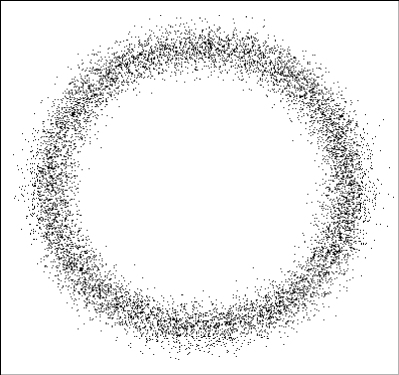
(a) Input density

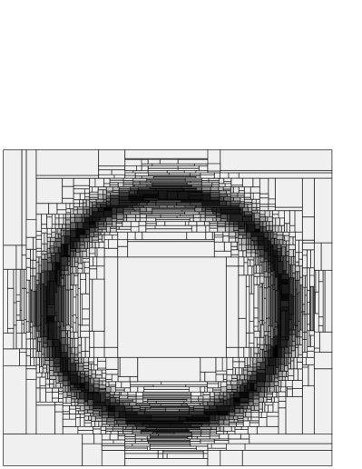
(b) Foam representation

Figure 2: (a) Two-dimensional Gaussian-ring distribution sampled from 500000 events. (b) Foam representation with 2000 active cells. The level of grey indicates the event density inside the corresponding cell.

The foam structure is formally equivalent to a decision tree [10]. The cut values of the decision tree correspond to the cell-splitting boundaries stored in the binary tree representing the foam. Optimisation of the decision tree (e.g. boosting) is replaced in case of PDE-Foam by the sampling and minimisation algorithm described above.

3.2 Foam Application for MVA

In order to use the Foam for MVA, two different concepts have been implemented:

1. Separate signal and background foams

   During the training phase two separate foams are created: one for signal and one for background events. The splitting of cells is based on the corresponding event densities. The number of signal (background) events contained in each cell of the final signal (background) foam is stored with the corresponding cell. During the classification phase the value of the discriminant for a given event x is calculated based on the number of events contained in the corresponding cells:

   $$D(\textbf{x})=\frac{n_{i}/V_{i}}{n_{i}/V_{i}+c\cdot n_{j}/V_{j}},$$ (7)

   where $n_{i}$ and $n_{j}$ are the number of events contained in cell $i$ of the signal foam and cell $j$ of the background foam, respectively, and $V_{i}$ and $V_{j}$ are the cartesian volumes of cell $i$ and $j$, respectively.

   The statistical uncertainty on the discriminant $\sigma_{D}(\textbf{x})$ is obtained in analogy to eq. 6.

2. One foam for discriminant distribution

   During the training phase one foam is created containing the distribution of the discriminant. The splitting of cells is based on the sampled discriminant distribution calculated according to the PDE-RS approach. Each cell $i$ contains a discriminant value $D_{i}$ calculated as:

   $$D_{i}=\frac{n_{s,i}}{n_{s,i}+c\cdot n_{b,i}},$$ (8)

   where $n_{s,i}$ ($n_{b,i}$) are the number of signal (background) events contained in cell $i$. The statistical uncertainty on the discriminant obtained in analogy to eq. 6 is also stored with each cell. During the classification phase the value of the discriminant for a given event $x$ from and independent testing sample and its statistical uncertainty are retrieved from the corresponding cell $i$.

For the same number of total foam cells, the performance of the two implementations was found to be similar.

3.3 Foam classification example

Figures 3(a)-(c) show the distribution of the discriminant for 500000 signal and 500000 background testing events of the Gaussian-ring example introduced above. The classification is performed with single discriminant foams of 100, 500 and 2000 active cells, respectively. The foams are created using 200000 signal and 200000 background training events. Besides the histograms for the events classified with PDE-Foam, also the corresponding curves for an analytical calculation are shown in the Figures.

For this example, both signal and background input distribution peak at the same values and are only distinguished by their different width. Therefore the resulting discriminant distributions for signal and background show a large overlap and poor separation.

The peaked structure of the histograms reflects the finite granularity of the foams. The distributions become smoother and approach the analytically calculated curves with increasing number of foam cells.

Figure 3(d) shows the resulting ROC curves for the same example. The curve for the theoretical optimum obtained from the analytical calculation is also shown. The area under the curve increases with increasing number of foam cells from 0.655 (100 cells) to 0.699 (2000 cells). The theoretical optimum corresponds to an area of 0.705. For a background rejection of 99%, the respective signal-efficiency values are between 1.5% (100 cells) and 1.85% (2000 cells) for the classification with PDE-Foam and 2.0% for the theoretical optimum.

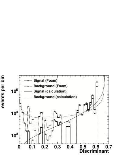
(a) Discriminant (100 cells)

(b) Discriminant (500 cells)

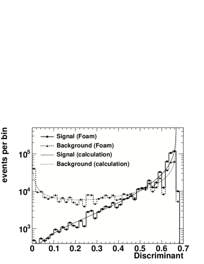
(c) Discriminant (2000 cells)

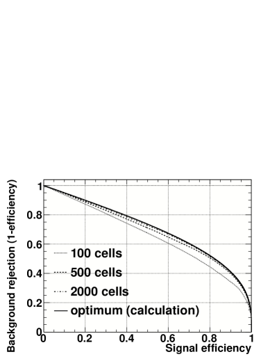
(d) Receiver Operating Characteristics

Figure 3: Distribution of the discriminant for signal and background events of the Gaussian-ring example using 100 (a), 500 (b) and 2000 (c) active cells, respectively. The curves overlaying the histograms show the distributions corresponding to an analytical calculation. The resulting ROC curves for the same example are shown in (d), together with the optimal curve obtained from the analytical calculation.

4 Implementation

The foam algorithm is implemented within the TMVA framework [7] as method PDE-Foam. The core foam functionality is inherited from the TFoam class included in ROOT [11]. Parameter steering, classification output and persistency mechanism follow TMVA standards, thus allowing to use it like other MVA methods implemented in TMVA and to compare the performance. The initial binary trees, which contain the training events, needed to evaluate the densities for the foam build-up based on the PDE-RS method, are discarded after the training phase.

The memory consumption for the foam is $160$ bytes per foam cell plus an overhead of $1.4$ kbytes for the PDE-Foam object on a $64$-bit architecture. Note that in the foam all cells created during the growing phase are stored within a binary tree structure. Cells which have been split are marked as inactive and remain empty. To reduce memory consumption, the geometry of a cell is not stored with the cell, but rather obtained recursively from the information about the division edge of the corresponding mother cell. This way only two short integer numbers per cell contain the information about the entire foam geometry: the division coordinate and the bin number of the division edge.

The foam object can be stored in XML or ROOT format. A projection method is available for visible inspection.

4.1 PDE-Foam parameters

Table 1 summarises the main PDE-Foam parameters that can be set by the user together with their default values. Optimisation of these parameters is needed to reach optimal classification performance. In the following, we discuss the dependence of the foam performance on the choice of parameters for some representative examples.

4.1.1 Size of sampling box

The size of the box used for the phase-space sampling is a common parameter of both the PDE-Foam method and the original PDE-RS method. In case of PDE-Foam, the box size is only relevant for the density sampling during the training phase, while for PDE-RS the box size is only used for the calculation of the discriminant during the classification phase. A larger box leads to a reduced statistical uncertainty for small training samples and to smoother sampling. A smaller box on the other hand increases the sensitivity to statistical fluctuations in the training samples, but for sufficiently large training samples it will result in a more precise local estimate of the sampled density.

Besides affecting the estimator performance, the box size influences the training time in case of PDE-Foam and the classification time in case of PDE-RS. A larger box increases the CPU time during sampling, due to the larger number of nodes to be considered in the binary search [6].

In general, higher dimensional problems require larger box sizes, due to the reduced average number of events per box volume. For uniformly distributed variables, the volume size containing a given number of events grows with the power of the number of dimensions. To collect 10% of the training events inside the sampling volume for a case with 10 variables, a box with edge length of 80% of the full range in each dimension is needed.

Figure 4 shows the estimator performance, measured as the area under the ROC curve, as function of the size of the sampling box and for examples with 2-10 observables (=dimensions). The examples are constructed as uncorrelated $n$-dimensional Gauss distributions with shifted means and different widths for signal and background.

The PDE-Foam performance (see Fig. 4(a)) is compared to the performance of the original PDE-RS method (see Fig. 4(b)). In both cases 50000 signal and 50000 background training events were used. For PDE-Foam, a target value of 1000 active cells was selected and a cut on the minimum number of events per cell of 100 (cf. discussion in section 4.1.3) was applied during the foam build-up. Here and in the following, the performance values have been obtained from independent testing samples of 500000 signal and 500000 background events.

The performance increases for both methods with the number of observables and with the size of the sampling box. It reaches a maximum for both methods, after which it drops again slightly with further increasing box size, due to the less precise local estimate of the larger boxes. PDE-Foam is less sensitive to statistical fluctuations in the training samples, due to the additional averaging stage during the density sampling inside the cells. Therefore the PDE-Foam performance reaches the optimum for smaller sampling boxes and has a wider range of stable performance, compared to the original PDE-RS implementation. For a small number of up to approximately four observables, there is almost no visible dependency of the performance on the box size. The default box size of 1/30 gives close to optimal results up to approximately five observables for this example. For the original PDE-RS method, on the other hand, a more careful optimisation of the box size is required, as the box size for optimal performance depends strongly on the number of dimensions and the convergence towards optimal performance is slower.

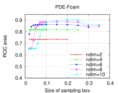
(a) PDE-Foam

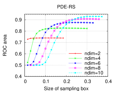
(b) PDE-RS

Figure 4: Dependence of the estimator performance on the size of the sampling box and the number of observables. The examples are constructed as Gaussian distributed observables with shifted means for signal and background and with variable number of observables. 50000 signal and 50000 background events each were used for the training phase. Shown are the performance for PDE-Foam (a) and for the original PDE-RS method (b).

4.1.2 Number of cells

The target number of cells for the final foam is the main parameter impacting the accuracy of the phase-space binning. An increased number of cells leads in general to improved performance provided that sufficiently large training samples are available. However, for an increasing number of cells with small training samples, the foam becomes more vulnerable to statistical fluctuations in the training samples in particular in less populated regions of the phase space and the performance might drop when further increasing the target number of cells (overtraining). Both the training time and the memory needed to store the foam object increase linearly with the number of cells, while the classification time scales approximately as $T_{class}\propto N_{cells}\cdot\log N_{cells}$.

Figure 5 shows the dependence of the estimator performance as function of the number of active cells for an example with five moderately correlated observables constructed from Gaussian distributions for signal and background. The two curves correspond to foams build-up from small and large training samples, respectively. The small training sample consist of 50000 signal and 50000 background events, whereas the large training sample contain 500000 signal and 500000 background events. No restriction on the number of events contained in each cell was applied.

As expected, the performance of the foams built from the large training sample exceeds the one of the foams based on the small training sample. In case of the large training sample, the performance for this particular example increases over a wide range of number of cells and reaches its maximum for about 20000 cells, after which it drops due to the decrease in statistical precision resulting in overtraining. For the small training sample, the maximum is already reached for foams with approximately 5000 cells and the drop in performance afterwards is steeper.

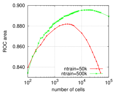
Figure 5: Dependence of the estimator performance on the number of active foam cells for an example with five moderately correlated observables constructed from Gaussian distributions and for two different training-sample sizes.

4.1.3 Minimum number of events

The cell splitting algorithm assumes sufficient statistical accuracy of the sampled density distributions in all cells. This might not be guaranteed in case of small training samples, where cell splitting in scarcely populated phase-space regions can lead to overtraining effects. Therefore cells should not be taken into account for further splitting, if the number of training events contained inside a cell is too small.

An adjustable parameter Nmin has been implemented, which sets the minimum number of events contained in any cell which is considered for further splitting. If the number of events is below Nmin, the cell is not considered for further splitting. If no more cells are available with sufficient number of events, the cell splitting stops, even if the target number of cells is not yet reached. Note that the Nmin requirement only affects the further splitting of cells. Therefore it is possible to have cells containing less than Nmin events in the final foam(s).

The cut on Nmin reduces the sensitivity to statistical fluctuations in the training samples and improves drastically the performance for small number of training events, as shown in Fig. 6(a) for the example with 5 observables and only 10000 training signal and background events each. Without the cut on Nmin, the foams with larger number of target cells suffer from overtraining and show a significantly decreased performance. Starting from a value of $\texttt{Nmin}\approx 8$, the effective number of final cells, as shown in Fig. 6(b) is limited to a value below 10000 and therefore the performance curves for 10000 and 30000 target cells become identical (Fig. 6(a)). For a value of $\texttt{Nmin}\approx 40$, this number drops to 2000 cells, visible in both figures as the points where all three curves merge. For very large values of Nmin the performance drops again, as the size of the few remaining cells becomes too large.

The default value of $\texttt{Nmin}=100$ leads to a good performance for most cases studied. It can be combined with a large target number of cells, as it limits the effective number of cells sufficiently and thus avoids overtraining even for small training-sample sizes. For the example shown in Fig. 6, the value of $\texttt{Nmin}=100$ corresponds to approximately 450 active cells in the final foams.

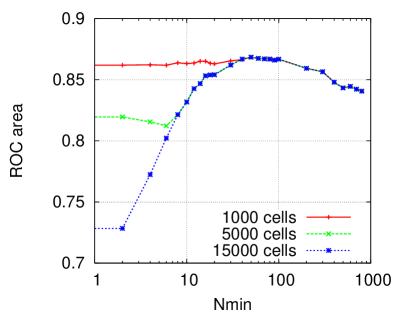
(a) Estimator performance

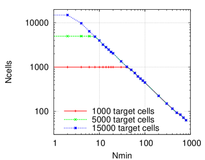
(b) Number of active cells in the final foam

Figure 6: Estimator performance (a) and number of active cells in the final foam (b) as function of the cut value for the minimum number of events per cell. The data shown corresponds to the example with five moderately correlated observables constructed from Gaussian distributions. It was calculated using 10000 signal and background training events each and target values of 1000, 5000 and 15000 active cells, respectively.

4.1.4 Number of samplings

The number of samplings per cell and cell-division step affects the phase-space sampling procedure during the foam build-up. The value has to be large enough to fill the density histograms used for the evaluation of the variance with sufficient statistical accuracy. On the other hand, increasing this parameter to a value much larger than the average number of training events contained in a cell will not improve the performance any further, as the sampling accuracy is limited in this case by the available number of training events in the cells. The foam build-up time scales approximately linearly with the number of samplings. The default value of 2000 is sufficiently large for optimal performance with all examples studied. For many cases with a small number of observables or small training-sample sizes, a reduced value of 500-1000 can be chosen without loss in performance.

4.1.5 Number of bins

Histograms are used to evaluate the variance across the cells projected on the cell axes. Cell splits are only performed at the bin boundaries. The accuracy of the determination of the division point increases with every iteration, as the histograms are refined with respect to the base cell after each division step. For all examples studied, the dependence both of the performance and the foam build-up time on the number of bins was found to be very small. The default value of 5 was found to be sufficient to achieve optimal performance.

4.1.6 Gaussian kernel smoothing

Foams with small number of cells and which are based on small training-sample sizes can suffer from large cell-to-cell fluctuations leading to large discontinuities at the cell boundaries. A Gaussian smearing can be applied during the classification phase to reduce the effect of these discontinouities [12]. In this case, all cells contribute to the discriminant calculation for a given event, convoluted with their Gauss-weighted distance to the event. The width parameter of the Gauss function used for the smearing is set to the length of the sampling box in each dimension (VolFrac).

Figure 7 shows the geometry of a foam with 250 active cells and the reconstructed event density, based on 5000 signal and 5000 background training events generated according to a two-dimensional Gaussian distribution with width 1.0 in each dimension and centred at (0.5,0). The reconstructed event densities with and without Gaussian kernel smearing are compared in Fig. 7(a) and 7(b). The width of the Gaussian kernel used for the smearing corresponds to 0.33 in the units of the original distributions. The improvement with kernel smearing is clearly visible. In most cases this procedure leads to an improved separation between signal and background.

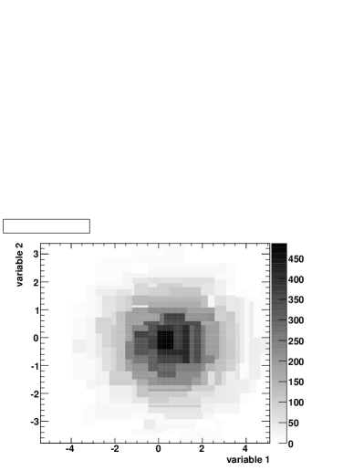
(a) Foam projection without kernel

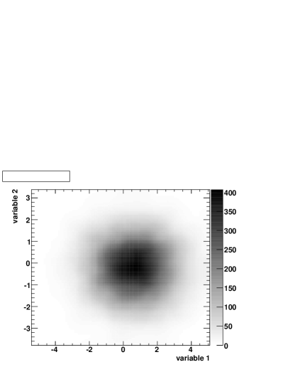
(b) Foam projection with Gaussian kernel

Figure 7: Foam representations of a two-dimensional foam with 250 active cells for a Gaussian distribution with width 1.0 in each dimension and centred at (0.5, 0). The foam was created with 5000 signal and 5000 background training events. (a) shows the event-density distribution without using kernel weighting and (b) shows the distribution after smearing with a Gaussian kernel of width 0.33. The level of grey indicates the event density inside the corresponding cell. The foam boundaries are rescaled to the coordinate system of the original observables.

Figure 8 shows the performance as function of the number of signal and background training events for an example with two-dimensional Gauss distributions and in comparison with the original PDE-RS method. Signal and background distributions have shifted means but identical widths in this example. The foams contain 250 active cells and a cut on the minimum number of events per cell was not applied. The Gaussian kernel smearing improves the performance, in particular for small training samples. For this example, it also exceeds the one of the original PDE-RS method. However, the Gaussian kernel smearing also largely increases the classification time. The classification times obtained using training signal and background samples of 100000 events each and testing signal and background samples of 500000 events each were approximately 1.5 min for PDE-RS, 1 min for PDE-Foam without Gaussian kernel smearing and 1 h for PDE-Foam with Gaussian kernel smearing.

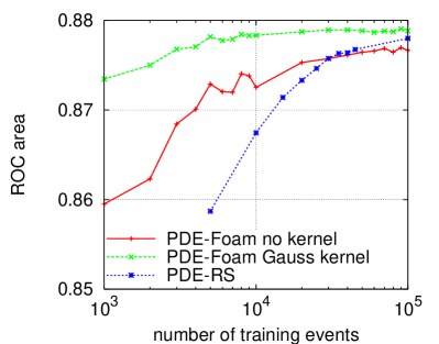
Figure 8: PDE-Foam performance as function of the number of training signal and background events for an example with two-dimensional Gauss distributions with shifted mean values for signal and background. Shown is the performance for a foam with 250 active cells, both without and with Gaussian kernel smearing during the classification phase. The performance of the original PDE-RS method is also shown for comparison.

5 Results

The two main limitations of the original PDE-RS method are:

• The performance of the PDE-RS method increases only slowly with the size of the training samples. For good results, typically large samples of the order of 500000 events are needed.

• Both the CPU time needed for classification and the memory consumption during classification increase with the number of training events. PDE-RS is therefore considered to be a slowly responding classifier for most applications.

In the following we present a comparison of the performance and CPU-time consumption between PDE-Foam and the original PDE-RS method. The results are shown for the example with five moderately correlated observables. Other examples have been studied and similar results were obtained.

5.1 Performance

Figure 9 shows the estimator performance as function of the number of signal and background training events for foams of 1000 and 20000 active cells, respectively. The left figure displays the area under the ROC curve as a performance measure, while the right figure shows the signal efficiency for a background rejection of 99%. The performance of the original PDE-RS method is also shown. Single foams were built for these examples with $\texttt{nSampl}=2000$ samplings, a sampling-box size of $\texttt{VolFrac}=1/30$ and a cut on the minimum number of events per cell of $\texttt{Nmin}=100$. In case of PDE-RS, the sampling-box size was 1.2 in units of the original observables, corresponding to approximately 0.12 in normalised coordinates.

For small training samples up to approximately 100000 events, the foams perform significantly better than the original PDE-RS method. Apparently the geometry of the foams is well adapted to the event distributions and the implicit averaging of the event densities over the cell volumes leads to better performance than the sampling with fixed box size performed by the original PDE-RS method. For training samples of less than 200000 events, the original PDE-RS method does not even reach a background rejection of 99%.

For very small training samples of 30000 events and less, the foams with 1000 and 20000 cells behave identically, since the cut on the minimum number of events per cell of 100 limits the effective number of final cells to a value below 1000.

For large training samples above 50000 events, the foam with 20000 cells performs better than the one with 1000, taking advantage of its finer granularity and the increased statistical precision of the larger training samples. However, for training-sample sizes of more than 200000 events, it does not quite reach the performance of the original PDE-RS method. For such large sample sizes, the local density estimates obtained with the PDE-RS method by counting events in the vicinity of the events to be classified are more precise than the density estimates from counting events in foam cells of finite granularity.

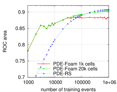
(a) ROC area

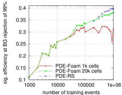
(b) Signal efficiency

Figure 9: ROC area (a) and signal efficiency at a background rejection of 99% (b) as function of the number of training signal and background events for the example with five moderately correlated observables constructed from Gaussian distributions. The performance for foams with 1000 and 20000 active cells are compared to the performance of the original PDE-RS method. The curve for PDE-RS in (b) starts from 200000 training events, as the method does not reach a background rejection of 99% for smaller training-sample sizes.

5.2 CPU time

Figure 10(a) shows the training time as function of the number of training signal and background events for foams of 1000 and 20000 active cells, respectively, for the example and parameters described above. The training time for the original PDE-RS method is also shown. For PDE-RS, the training time consists only of the creation of the binary-search trees used to store the training samples. For PDE-Foam, the training time is dominated by the repeated density sampling during the iterative build-up of the foam structure. Therefore the training time is larger than for the PDE-RS method. The training time for small training samples is identical for the foams with 1000 and 20000 cells, due to the cut on Nmin.

Figure 10(b) shows the CPU time used for classification of 500000 signal and 500000 background testing events as function of the number of signal and background training events. For the foams, the classification time depends mostly on the number of cells in the final foam and is almost independent of the number of training events. The slight variation with the number of training events is due to the corresponding increase of the number of cells and due to slight variations of the foam geometry. For the original PDE-RS method, on the other hand, the classification time rises with the number of training events, due to the larger size of the binary trees. For $10^{6}$ signal and background training events each, the classification time reaches approximately 40 minutes for PDE-RS, while for the foams with 20000 cells it is below 3 minutes. On the other hand, for small training samples of less than approximately 30000 events, the recursive reconstruction of the foam geometry during classification takes longer than the density sampling within the PDE-RS binary tree.

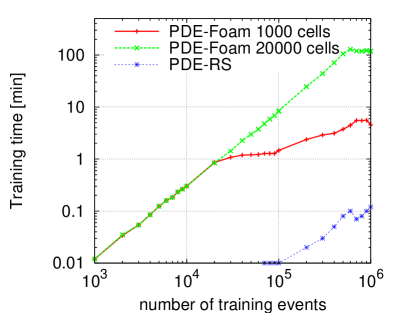
(a) Training time

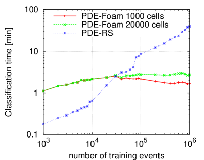
(b) Classification time

Figure 10: CPU time for training (a) and classification of 500000 testing events (b) as function of number of training events for a model with five observables. The CPU time for foams with 1000 and 20000 cells are compared to the performance of the original PDE-RS method.

6 Reconstruction of event quantities

The foam can be extended to reconstruct event quantities (regression analysis). In this case $n_{t}$ target values depend on $d$ observables. Two different methods have been implemented: the first method stores a single target value in every foam cell. The second method saves the target values in further foam dimensions. Since the first method can only be used if only one target is given, it is called ’Mono target regression’. In order to do regression with multiple targets one has to use the second method, called ’Multi target regression’.

In case of the mono-target regression, the density $\rho$ used during the foam build-up phase, is given by the mean target value $\langle t\rangle$ within the sampling box, divided by the box volume (given by the VolFrac option):

$$\rho=\frac{\langle t\rangle}{\texttt{VolFrac}^{d}}\equiv\frac{\sum_{i=1}^{N_{b}}t^{(i)}}{N_{b}\times\texttt{VolFrac}^{d}},$$ (9)

where the sum goes over all events $N_{b}$ within the sampling box and $t^{(i)}$ is the target value of the event ${\textbf{x}}^{(i)}$ ($i=1,\ldots,N_{b}$). During the foam build-up phase, the relative variance of the density $\sigma_{\rho}/\langle\rho\rangle$ is minimised in the same way as described in section 3.1.

After build-up of the foam, each cell is filled with the average target value. During classification the target value is estimated for any given event x and is given as the content of the corresponding foam cell.

In case of multi-target regression, the $n_{t}$ target values are treated as additional dimensions during the foam build-up. The density used for the foam build-up is estimated from the number of events in a box of fixed size in the $d+n_{t}$-dimensional phase space. The number of events contained in the volume of each cell of the final foam is stored with the foam. The target values for any given event x are estimated as the projections of the centre of the corresponding cell onto the corresponding axes formed by the $n_{t}$ target values.

Figure 11(a) shows the geometry and the target density for a mono-target foam with 1500 active cells, calculated for an example with two observables and a quadratic dependence of the target value $t$ on two uniformly distributed observables, $\textrm{x}_{1}$ and $\textrm{x}_{2}$:

$$t=a\cdot\textrm{x}_{1}^{2}+b\cdot\textrm{x}_{2}^{2}+c+\Delta t,$$ (10)

where $a$, $b$ and $c$ are constant and $\Delta t$ is a small random number simulating noise. The accuracy of the event reconstruction with this foam is shown in Fig. 11(b), where the relative difference between the reconstructed and true target value is displayed. The mean value is reconstructed with an accuracy of approximately 0.5 per mille. The RMS of the distribution is about 3%. Also shown in the figure is the relative difference between the generated events before and after adding the noise term. The width of this distribution is approximately 0.7%. It can be considered as the optimal value for the accuracy of the event reconstruction.

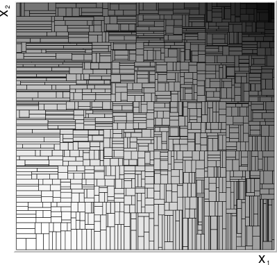
(a) Foam geometry and target density

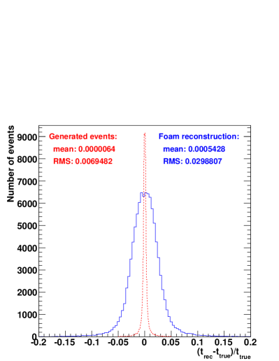
(b) Accuracy of event reconstruction

Figure 11: Mono-target regression for a bivariate quadratic target function. (a) shows the geometry and target density of the resulting foam with 1500 active cells. The level of grey indicates the target density inside the corresponding cell. In (b) the dashed line shows the relative difference between the generated events before and after adding the noise term and the solid line shows the accuracy of the event reconstruction with PDE-Foam.

7 Conclusions

A new method for multi-variate analysis, PDE-Foam, has been developed. It combines the adaptive binning algorithm of the Foam method so far only used for Monte-Carlo event generation with probability density estimation based on range searching. PDE-Foam has been implemented within the TMVA package for multi-variate analysis.

We demonstrated that the default set of foam build-up parameters leads to robust results for the various examples studied and we gave guidance for further parameter optimisation. We showed that the performance of PDE-Foam exceeds the classification performance of the original PDE-RS method for small training samples. Furthermore, it leads to largely reduced classification time. Both the classification time and the memory consumption are independent of the number of training events. The main limitations of the original PDE-RS implementation have therefore been overcome.

In addition to event classification we have implemented a method to reconstruct event quantities with PDE-Foam.

References

- [1] C. M. Bishop, Pattern Recognition and Machine Learning, Springer, New York, USA (2006) and references therein.
- [2] L. Holmström, S.R. Sain and H.E. Miettinen, Comput. Phys. Commun. 88 (1995) 195.
- [3] The H1 Collaboration, C. Adloff et al., Eur.Phys.J. C 25 (2002) 495-509.
- [4] The ZEUS Collaboration, S. Chekanov et al., Phys. Lett. B 583 (2004) 41.
- [5] The ATLAS Collaboration, G. Aad et al., Expected Performance of the ATLAS Experiment: Detector, Trigger and Physics (Chapter on Tau reconstruction), CERN-OPEN-2008-020 (2008) [arXiv:0901.0512].
- [6] T. Carli and B. Koblitz, Nucl. Instr. and Meth. A 501 (2003) 576.
- [7] A. Höcker et al., PoS ACAT (2007) 040 [arXiv:physics/0703039].
- [8] S. Jadach, Comput. Phys. Commun. 130 (2000) 244; S. Jadach, Comput. Phys. Commun. 152 (2003) 55.
- [9] J. Neyman and E. S. Pearson, Philos. Trans. R. Soc. London A 213 (1933) 289-337.
- [10] L. Breiman, J.H. Friedman, R.A. Olshen, and C.J. Stone, Classification and Regression Trees, Wadsworth International Group, Belmont, USA (1984).
- [11] R. Brun and F. Rademakers, Nucl. Instr. and Meth. A 389 (1997) 81-86. See also http://root.cern.ch/.
- [12] K. S. Cranmer, Comput. Phys. Commun. 136 (2001) 198-207.